Flexible neural control of motor units

Abstract

Voluntary movement requires communication from cortex to the spinal cord, where a dedicated pool of motor units (MUs) activates each muscle. The canonical description of MU function rests upon two foundational tenets. First, cortex cannot control MUs independently but supplies each pool with a common drive. Second, MUs are recruited in a rigid fashion that largely accords with Henneman’s size principle. While this paradigm has considerable empirical support, a direct test requires simultaneous observations of many MUs across diverse force profiles. We developed an isometric task that allowed stable MU recordings, in a rhesus macaque, even during rapidly changing forces. Patterns of MU activity were surprisingly behavior-dependent and could be accurately described only by assuming multiple drives. Consistent with flexible descending control, microstimulation of neighboring cortical sites recruited different MUs. Furthermore, the cortical population response displayed sufficient degrees of freedom to potentially exert fine-grained control. Thus, MU activity is flexibly controlled to meet task demands and cortex may contribute to this ability.

Introduction

Primates produce myriad behaviors, from acrobatic maneuvers to object manipulation, all requiring precise neural control of muscles. A muscle is controlled by a motor neuron pool (MNP) containing hundreds of α-motoneurons, each innervating a unique subset of muscle fibers. A motoneuron and associated fibers constitute a “motor unit” (MU)¹. MUs are heterogeneous, differing in size (large MUs innervate more fibers)², duration of generated force³, and muscle length where force becomes maximal⁴.

Optimality suggests flexibly using MUs suited to each situation^5–7. Yet nearly a century of research supports an alternative rigid strategy that approximates optimality^1,8,9. With limited exceptions, MUs within a pool are believed to be recruited in a consistent order^10,11 from smallest to largest, obeying Henneman’s size principle^12–17. Small-to-large recruitment minimizes force fluctuations¹⁸ and energy expenditure¹⁹, and is attributed to intrinsic motoneuron properties^1,9. Rigid recruitment is computationally efficient²⁰: one ‘common drive’ determines every MU’s activity²¹. Henneman found small-to-large recruitment regardless of whether input was delivered via electrical stimulation of dorsal roots¹²; electrical stimulation of the motor cortex, basal ganglia, cerebellum, or brain stem²²; or mechanical activation of reflex circuits¹³.

Rigid recruitment is believed to simplify control (Fig. 1a). If “the brain cannot selectively activate specific motor units¹”, it is freed from the need to do so. Instead, each MU’s activity is a fixed function of a unified force command, yielding small-to-large recruitment with limited well-established exceptions. It is cautioned that these exceptions should not be misinterpreted as flexibility^23–26. First, conduction-velocity differences impact recruitment order during ballistic contractions^8,23. Second, cell-intrinsic mechanisms cause some MUs to rotate on and off, over many seconds, to combat fatigue²⁷. Finally, for ‘multifunctional’ muscles with multiple mechanical actions, the size principle holds only within each action^6,28,29. Each mechanical action is hypothesized to have its own common drive (or ‘synergy’). These drives overlap imperfectly within the MNP³⁰ (Fig. 1a, middle) and are preferentially reflected by different nerve branches³¹. Recruitment is still considered rigid²⁵ because it is a fixed function of a small number of commands.

Figure 1 |. Rigid versus flexible motor unit control and experimental setup.

(a) Rigid control schematic. The activity of many MUs is determined by a small number of force commands. Commands may be for individual-muscle force, or may be ‘synergies’ that control a mechanical action (e.g., an elbow flexion synergy and a forearm supination synergy). Thus, the number of controlled degrees of freedom is less than or equal to the number of motor neuron pools. Each MU’s activity is a ‘link function’ of one synergy (or for multifunctional muscles, 2–3 synergies). Link functions typically enforce size-based recruitment. (b) Flexible control schematic. Each motor neuron pool is controlled by multiple degrees of freedom, such that recruitment can be size-based but can also be flexibly altered when other solutions are preferable. (c) Task schematic. A monkey modulated the force generated against a load cell to control Pac-Man’s vertical position and intercept a scrolling dot path. (d) Single-trial (gray), trial-averaged (black), and target (cyan) forces from one session. Vertical scale: 4 N. Horizontal scale: 500 ms.

The opposite of rigid control -- highly flexible control that leverages many degrees of freedom (Fig. 1b) -- has rarely been considered viable. EMG frequency analysis suggests flexibility⁷ within the rat gait cycle³² and across cycling speeds in humans³³. Yet most studies argue that speed-based recruitment is absent^23,34 and/or of limited benefit³⁵. Thus, the consensus has been that speed does not reveal flexibility^1,25,36,37. A possible exception is fast lengthening contractions⁵, but studies disagree³⁸ regarding whether this is a general property³⁶. Latent flexibility is suggested by biofeedback training^26,39,40 yet may be limited⁴¹ and could involve known phenomena including multifunctional muscles²⁴. The prevailing view is thus that flexibility is likely scant^36,37 or non-existent²⁵. Yet many have stressed the need for further examination using improved recording techniques⁷ and a broader range of behaviors²⁵.

Results

Pac-Man Task and EMG recordings

We trained a rhesus macaque to perform an isometric force-tracking task. Force controlled a ‘Pac-Man’ icon that intercepted scrolling dots (Fig. 1c). The dot path instructed force profiles (Fig. 1d, cyan). Actual forces (single trials in gray) closely matched target profiles. We performed three experiment types across 38 ~1 hour sessions. Microstimulation experiments perturbed descending commands. Dynamic experiments employed diverse force profiles. Muscle-length experiments used multiple force profiles across two muscle lengths.

In each session, we recorded from multiple custom-modified percutaneous thin-wire electrodes closely clustered within one muscle head. EMG spike-sorting is notoriously difficult during dynamic tasks; movement threatens stability and vigorous activity produces superimposed waveforms. Three factors aided spike sorting: the isometric task facilitated stability, the number of active MUs could be titrated via task gain, and each MU produced a complex waveform spanning multiple channels (Extended Data Fig. 1). We adapted recent spike-sorting advances, including methods for resolving superimposed waveforms. We isolated 3–21 MUs per session (356 total). To eliminate the possibility that recruitment might mistakenly appear flexible due to properties of multifunctional muscles, forces were all generated with the same mechanical action. Furthermore, recordings included non-multifunctional muscles and analyses considered only simultaneously recorded neighboring MUs.

Cortical perturbations

If rigid MU control is spinally enforced¹³, artificially perturbing cortex should modulate MU activity while preserving orderly recruitment²². In contrast, if control is flexible, cortex might participate and perturbations might drive diverse recruitment patterns. It is argued that this does not occur²², but the possibility is suggested by a mapping study in baboons⁴². To investigate, we delivered microstimulation in sulcal motor cortex (Fig. 2a), during static forces, while recording from the deltoid, triceps, and pectoralis (18 sessions with 6661 total successful trials; 183 total MUs, 3–21 per session). We compared stimulation-driven responses amongst neighboring cortical electrodes. We also recorded during a four-second force ramp without stimulation.

Figure 2 |. Stimulation experiments.

(a) Microstimulation was delivered, on interleaved trials, through a selection of electrodes on a linear array. (b) EMG voltages for two EMG recording channels (of eight total) and four example trials, stimulating on electrode 23 or 27. The two electrodes recruited MUs with different waveform magnitudes, and vertical scales are adjusted accordingly. Stimulation was delivered during each green-shaded region, during which a small stimulation artifact can be seen. Right. spike templates for these two MUs. Vertical scale: 50 standard deviations of background noise (ignoring stimulation artifact). (c) Responses of the same two MUs, for all trials during stimulation on three electrodes. Traces plot firing rates (mean and standard error). Rasters show spike times, separately for the two MUs. (d) As in c but for a different session. (e) Additional example from a different session, showing responses during both the four-second ramp and during stimulation as the monkey held two baseline force levels. Mean force plotted at top. (f) As in e, but for a different session. (g) State-space predictions for rigid control (left) and flexible control (right). (h) State-space plots for two sessions where MUs were recorded from the lateral deltoid. Each subpanel plots joint activity of two MUs during stimulation on each of three electrodes. (i) For two sessions recording from sternal pectoralis major. Left: activity during stimulation on three electrodes. Right: activity during stimulation on two electrodes and during the slow force ramp. (j), For two sessions recording from lateral triceps.

Rigid control is fundamentally a hypothesis regarding the population response. Yet if activity departs from rigid control, there should exist pairwise comparisons (amongst just two MUs) where flexibility becomes patent. Pairwise comparisons are helpful because inspection at the level of spikes and rates allows one to consider trivial explanations. In Fig. 2b, stimulation recruited two neighboring pectoralis MUs, visible on the same channels (MU206’s waveform is smaller and shown on an expanded scale). Cortical electrode 23 primarily recruited MU206. Electrode 27 (400 microns away) primarily recruited MU215. This effect was robust across trials (Fig. 2c). Electrode 24 (physically between 23 and 27) recruited both. These observations are incompatible with electrodes 23 and 27 recruiting the same common drive. Effects cannot be due to sampling error; standard errors of the mean are small. A similar effect is illustrated for two triceps MUs (Fig. 2d). Such effects were common: in 13/18 sessions, the relative activation of MUs depended on which electrode delivered stimulation (ANOVA, interaction between MU identity and electrode; p < 0.001 adjusted for multiple comparisons; N = 11–77 trials per condition; session average = 29).

Cortical stimulation also yielded departures from the natural recruitment observed during the force ramp. For example, based on responses during the ramp, MU295 has a higher recruitment threshold than MU289 (Fig. 2e, left). Yet electrode 24 activated only MU295 (Fig. 2e, middle). When MU289 was already active during static force production (Fig. 2e, right), stimulation had an effect consistent neither with common drive (it differed for the MUs) nor with recruitment during the ramp.

Departures from rigid control were not due to small latency differences amongst MUs²³. For example, in Fig. 2c,d, all key departures relate to magnitude not latency. The same is true in Fig. 2e,f. Still, small latency differences exist: e.g., MU206 rises ~20 ms earlier than MU215 (Fig. 2c). Subsequent quantification thus takes latency into account. We saw little evidence for fatigue over a session, both in individual-example rasters and in summary analysis (Extended Data Fig. 2b). Occasionally, fatigue-combatting rotations²⁷ produced ‘streaky’ spike rasters (Fig. 2f, red) but this did not create the departures from rigid control in trial-averaged rates. To minimize any impact of fatigue-related effects, trials for all conditions (including stimulation sites) were interleaved. Occasionally, cortical perturbations produced hysteresis (Fig. 2f, right), likely reflecting persistent inward currents⁴³. Unlike the immediate effect of stimulation, hysteresis rarely altered recruitment relative to natural behavior, consistent with properties of persistent inward currents³⁷.

State-space predictions of rigid control

The hypothesis of rigid control is naturally expressed in a state space where every MU contributes an axis. Each MU’s activity is a monotonic function (termed a ‘link function’) of common drive^44,45. Thus, with increasing drive, population activity should move farther from the origin, tracing a monotonic one-dimensional (1D) manifold (Fig. 2g, left). The manifold may curve (due to nonlinear link functions) but greater drive should cause all rates to increase (or remain unchanged if maximal or not yet recruited). In contrast, flexible control predicts recruitment patterns unconfined to a monotonic 1D manifold (Fig. 2g, right). We use MU pairs to illustrate. Responses sometimes adhered to rigid-control predictions (Fig. 2h, left). Yet stimulation on different electrodes often yielded different trajectories (Fig. 2h, right; Fig. 2i,j), as did activity during the ramp. Brief trajectory ‘loops’ likely reflect small latency differences and are thus compatible with rigid control. In contrast, entirely different trajectory directions are not.

Standard statistical tests (e.g., the ANOVA above) ask when MU responses are statistically different. However, the key population-level question is not whether responses differ, but whether differences can be explained by different link functions operating upon a common drive. Before engaging in model fitting, a simpler approach is to leverage the state-space perspective and ask whether population trajectories are logically consistent with rigid control. To do so, we applied a novel metric: ‘MU displacement’ (Fig. 3a). Suppose two MUs have rates of 10 spikes/s at time t. If both rates increase by time t’ (possibly within a different condition), one can connect them with a monotonic manifold (left, dashed line). This is not true if rates change in opposition (right). ‘Displacement’ (blue) is the smallest alteration, in either MU’s rate, that renders activity consistent with a monotonic manifold. For each population response (one per session) we identified the MU pair causing the largest displacement, then minimized this displacement by allowing temporal shifts to eliminate latency-based effects. Any remaining displacement was the maximal displacement for that session. For 16/18 sessions, maximum displacement was higher than expected from sampling error (Fig. 3b, p<0.001, two-sample t-test). Displacements were larger when considering population trajectories across all stimulation sites (“all-stim”) versus each site alone (“1-stim”). This agrees with the ANOVA above: different stimulation sites often drove different MU-activity patterns. Even within a site, displacement was occasionally non-negligible, indicating some MUs displayed responses with opposing polarities or temporal patterns. We extended the “all-stim” analysis by removing, from the population, the MU pair responsible for the largest displacement. We recomputed displacement and iterated until remaining displacement was no larger than the largest expected from sampling error (Fig. 3c). On average it was necessary to remove 6.2 MUs, out of an average of 10.2 per session. Thus, a reasonably large percentage of the MU population showed responses inconsistent with rigid control.

Figure 3 |. Quantifications of flexible control.

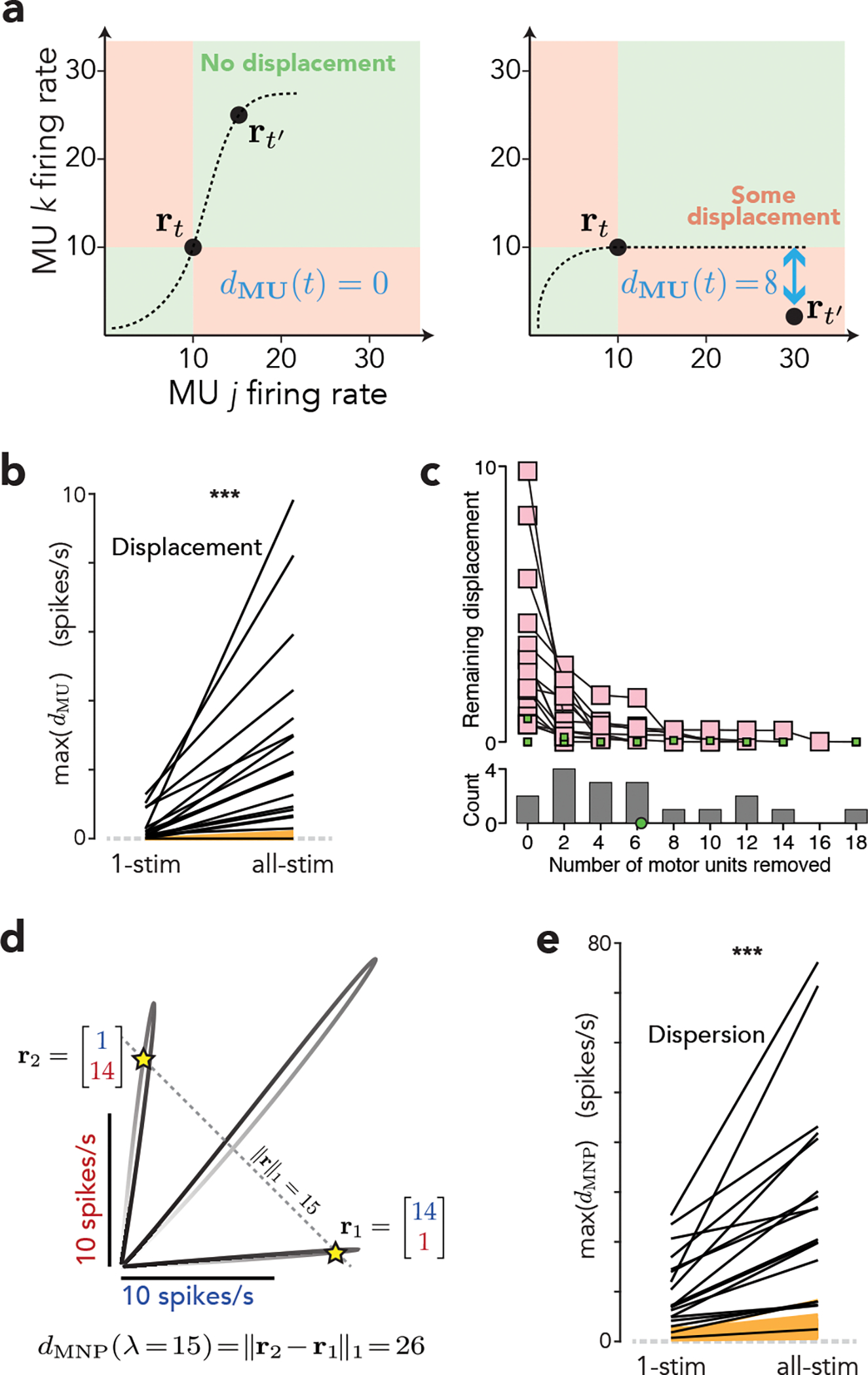
(a) Schematic illustrating MU displacement (d_MU) for a two-dimensional population state and two times. Left. a monotonic manifold can pass through r_t and ${\mathbf{r}}_{t^{\prime }}$. Thus, d_MU(t) = 0. Right. Any monotonic manifold passing through r_t is restricted to the green zone, and thus cannot come closer than 8 spike/s to ${\mathbf{r}}_{t^{\prime }}$. Thus, d_MU(t) = 8. (b) Maximum displacement (one black line per session). For ‘1-stim’, displacement was computed across times during the response for each stimulation site alone. The maximum was then taken across sites from that session. For ‘all-stim’, the maximum displacement was computed across all times and stimulation sites within a session. ‘All-stim’ displacement was significantly larger (two-sample two-tailed t-test, p = 0.00017, N=18 sessions). Both were significantly larger than the displacement expected due to sampling error alone (yellow, ten resampled artificial populations per empirical dataset). (c) Maximum displacement (for ‘all-stim’) after repeatedly removing the MU pair causing the largest displacement. Each trace corresponds to one session, and ends when remaining displacement is no larger than the largest across the ten resampled populations for that session. Gray histogram plots the distribution, across sessions, of the number of MUs that had to be removed to reach that point (mean in green). (d) Illustration of MNP dispersion metric for two MUs. The three trajectories were driven by stimulation at three cortical sites. The line defined by ∥r∥₁ = 15 intercepts these trajectories at six points, with r₁ and r₂ being most distant. The MNP dispersion for λ = 15 is the L1 distance between these points. (e) Maximum (across λ) dispersion (one line per session). ‘All-stim’ dispersion was significantly larger (two-sample two-tailed t-test, p = 0.00011, N=18 sessions). Both were significantly larger than the dispersion expected due to sampling error alone (yellow, ten resampled artificial populations per empirical dataset). Results are shown for conditions where stimulation was delivered as the monkey held a low static force, and were nearly identical for a higher static force.

We also applied a related metric, ‘MNP dispersion’. As common drive increases, so should the summed activity of all MUs: the L1-norm, ∥r∥₁. Thus, there should not be two different ‘ways’ of achieving a given ∥r∥₁. Geometrically, crossing a given diagonal in multiple places (Fig. 3d) is incompatible with a monotonic manifold. We defined MNP dispersion, d_MNP(λ) as the maximum distance between all population states with norm λ. For each population we computed the maximum dispersion (across λ), then minimized that value by allowing latency shifts. In agreement with analyses above, dispersion was largest when considering all stimulation sites (Fig. 3e). Dispersion exceeded that expected given sampling error for 17/18 sessions (Fig. 3e).

Optimal motor unit recruitment

Is the capacity for flexible MU recruitment used during behavior? Because larger MUs tend to generate shorter-lived forces⁴⁴, a venerable suggestion is that flexibility might reveal itself when comparing slow versus fast movements^5,7,32,33. The prevailing view is that this does not occur¹. Recruitment is preserved during slowly and quickly increasing force ramps²³, excepting trivial latency effects. Yet studies have found evidence for flexible recruitment^5,33 using non-ramping force profiles. We reasoned that revisitation of this topic would benefit from clear expectations regarding which force profiles are most likely to evoke altered recruitment.

We developed a simplified computational model, inspired by prior work that established size-based recruitment as the optimal fixed strategy^18–20. We inquired how recruitment would behave were it infinitely flexible and optimized for each force profile. We modeled the force produced by an idealized MNP with N MUs as

$$f_{\text{MNP}}(t)=\sum _{i=1}^N\left(h_i*r_i\right)(t)$$ (1)

where h_i(t) is the twitch responses (modeled as in⁴⁴) and r_i(t) is the idealized firing rate of the i^th MU. Twitch responses were bigger and briefer for larger MUs. For each target-force profile, we optimized MU rates (Fig. 4a) to minimize error (both average error and trial-to-trial variability) between f_MNP(t) and intended force (Fig. 4b). Optimization considered the entire force profile, and could thus consider whether a force would be short-lived.

Figure 4 |. Optimal MU recruitment.

(a) Isometric force production was modeled using an idealized MNP containing 5 MUs. MU twitch amplitude varied inversely with contraction time such that small MUs were also slow. A given set of rates resulted in both a mean total force and inferred trial-to-trial variation around that force. The latter was smaller when using multiple small MUs versus one large MU. Both contributed to mean-squared error between actual and target forces. The optimal set of MU firing rates was numerically derived as the solution minimizing that error. Optimization was independent for each force profile. (b) Example target (cyan) and mean MNP (black) forces (for simplicity no variability is shown). Mean force matched targets very well, with notable small exceptions at the troughs during sinusoidal forces. (c) Optimal MU firing rates, used to generate the forces in b. Each color corresponds to a different MU, numbered by size (MU1 was the smallest and slowest). (d) State space plot of MU3 versus MU2 for each condition in c.

Recruitment (Fig. 4c) was purely size-based for slowly ramping forces. Recruitment departed from purely size-based during fast ramps, but only modestly. Were such deviations observed empirically, most would be indistinguishable from latency differences. Recruitment was more profoundly altered during fast sinusoids. A similar effect was observed within chirps; recruitment changed as frequency increased. State-space plots confirm that, even under the assumption of complete flexibility, activity followed a similar manifold for slow and fast ramps (Fig. 4d). In contrast, flexibility revealed itself when comparing between slow ramps and the high-frequency sinusoid, or within the chirp. Flexibility leverages the fact that preferentially using small (slow) MUs minimizes fluctuations^18,20. However, for high-frequency sinusoids, it becomes optimal to rely more on large (fast) MUs to avoid excessive force during troughs.

Motor unit activity across force profiles

Using diverse force profiles that included sinusoids (Fig. 1d) we recorded MU populations from the deltoid and triceps (14 sessions with 4734 total successful trials; 134 total MUs, 3–20 MUs per session). MUs showed a range of recruitment thresholds and peak rates (Extended Data Fig. 2a). There was no indication of general fatigue across a session (Extended Data Fig. 2b). As predicted by the optimal-recruitment model, MU recruitment differed between slowly changing forces and high-frequency sinusoids. For example, in Fig. 5c, three lateral triceps MUs are active during the four-second ramp (left). During the 3 Hz sinusoid, these MUs are similarly (or slightly less) active, and are joined by MUs that are active primarily during the sinusoid (right). Extended Data Fig. 3 shows additional single-trial traces, and rasters for all trials / MUs from this session. Of seven recorded MUs, three were strongly active during the 3 Hz sinusoid despite being inactive during the ramp.

Figure 5 |. Dynamic experiments.

(a) Forces for two conditions: the four-second ramp and the 3 Hz sinusoid. Gray traces show all trials in this session. Black traces highlight trials for which EMG data are shown below. (b) MU spike templates across four (of eight) EMG channels recorded in the lateral triceps. Vertical scale: 50 standard deviations of the noise. Each template spans 10 ms. (c) EMG voltage traces for the two trials and time-periods highlighted in a. Traces become colored to indicate when spikes were detected. Numbers indicate the identity of the MU producing the spike. In some cases, spikes from two or more MUs overlap. Trace color reflects the relative magnitudes of the contributions made by different MUs. (d) Responses of two MUs during the 0.25 Hz sinusoid. Black trace at top shows trial-averaged force. Colored traces show firing rates (mean and standard error). Rasters show individual spikes on all trials for these conditions. Vertical scales: 8N and 20 spikes/s. (e) Response of two MUs during the four-second ramp (left) and 3 Hz sinusoid (right). MU311 and MU309 correspond to MUs 3 and 5 for the session focused on in c. (f) Response of two MUs (from a different session) during the four-second ramp (left) and the 0 – 3 Hz chirp (right). (g) Response of two MUs (from a different session) during the 250 ms increasing and decreasing ramps. (h,i,j) State-space plots for the MUs shown in d,e,f. Scale bars: 20 spikes/s. (k) Maximum displacement for every session. Displacement was computed twice: within the four-second ramp only, and again across all conditions. Yellow lines plot displacement expected due to sampling error (ten resampled artificial populations per session). Empirical slopes were significantly larger than expected given sampling error (two-sample two-tailed t-test, p = 0.000003, N=14 sessions). (l) Maximum displacement, across all conditions, after repeatedly removing the MU pair that caused the largest displacement. Each trace corresponds to one session, and ends when remaining displacement was no larger than the largest from the ten resampled datasets (or when no pairs would be left). Gray histogram plots the distribution, across sessions, of the number of MUs that had to be removed (mean in green). One session (lone green square) terminated immediately because it contained only 3 MUs. (m) Cumulative distribution for displacement (d_MU(t)). Rather than summarizing a session by taking the maximum across all times (as in k,l), here we plot the distribution of d_MU(t) for all times within one session. Distributions were computed for the slowly increasing ramp alone (purple) and all conditions (green). (n) Maximum (across λ) dispersion (one line per session). Slopes were significantly larger than expected given sampling error (two-sample two-tailed t-test, p = 0.0000007, N=14 sessions). (o) Additional within-session analysis of dispersion. Rather than summarizing a session by taking the maximum d_MNP(λ) across λ (as in n), here we plot d_MNP(λ) versus the λ (the norm).

Inspection of examples illustrates a range of effects. When considering only slowly changing forces (Fig. 5d), activity was equally consistent with rigid versus flexible control. Activity became inconsistent with rigid control when also considering high-frequency sinusoids. For example, MU309 (Fig. 5e) becomes far more active during the fast sinusoid, even as MU311 becomes slightly less active (these correspond to MU5 and MU3 from panel c). MU329 (Fig. 5f) is inactive during the four-second ramp and early in the chirp, but becomes active for the higher-frequency cycles even as MU324’s rate declines.

Both prior work and the optimal-recruitment model argue against large recruitment differences between slow and fast ramps. Indeed, despite their high rate of change (~64 N/s), fast (250 ms) ramps rarely produced recruitment that was clearly different from four-second ramps. The only compelling exceptions were at force offset. For example, MU109 (Fig. 5g) tripled its activity in anticipation of a fast downward ramp, even as MU108 became slightly less active. A similar but smaller effect is exhibited by the model: large/fast MUs start to ‘take over’ so force can terminate swiftly (in follow-up simulations, moving to even faster offsets enhanced this strategy).

As above, inspection of examples is useful when considering alternative explanations. Departures were not explained by some MUs reflecting force while others reflected its derivative. For example, MU309 (Fig. 5e) and MU329 (Fig. 5f) are more active during higher-frequency forces, but do not phase lead their neighboring MUs. Furthermore, responses did not exhibit large overshoots during rapidly increasing ramps (e.g., Fig. 5g, left). Effects were also not explainable by some sort of rapid within-trial fatigue. For example, there is no evidence of fatigue in Fig. 5e. In Fig. 5f, one might propose that MU324’s rate declines during the chirp due to fatigue, yet it maintained a consistently high rate during the much longer ramp. In Fig. 5g, the departure occurs because activity increases (not fatigues) in anticipation of force offset. Still, some MUs did show a slight rate ‘sag’, especially during the lengthy four-second ramp (Fig. 2e, left). These long-timescale effects are presumably not a meaningful departure from rigid control, something taken into account when interpreting quantitative analyses below. We occasionally observed fatigue-combatting rotations; an MU could become less active for a handful of trials. To reduce any condition-specific impact on trial-averaged rates, trials for all conditions were interleaved. Inspection of individual-MU responses (also see Extended Data Fig. 3) confirms that different recruitment between ramps and sinusoids cannot be attributed to rotations or other long-timescale fatigue-related effects.

In situations where activity was potentially consistent with rigid control (Fig. 5d), trial-averaged trajectories hewed close to a monotonic manifold (Fig. 5h). When activity was incompatible with rigid control (Fig. 5e,f), trajectories diverged from a monotonic manifold (Fig. 5i,j). To quantify at the population level, we employed the displacement and dispersion metrics. We focused on the model-based prediction that departures from rigid control should be minimal during the four-second ramp (where rigid and flexible control predict the same small-to-large strategy) but become common when considering all conditions. The four-second ramp is also a useful comparison because it provides an estimate of trivial departures from idealized rigid control due to modest temporal instabilities. Indeed, during the four-second ramp, displacement (Fig. 5k) and dispersion (Fig. 5n) were small but higher than expected given sampling error (yellow lines). Inspection of individual cases revealed that such effects were ‘real’ but not evidence of flexibility; they reflected uninteresting phenomena such a slight sag in rate over long timescales (as in Fig. 2e, left).

When considering the population response across all conditions, displacement (Fig. 5k) and dispersion (Fig. 5n) became much larger (p<0.001). All 14 sessions had a maximum displacement outside the range expected due to sampling error. As above, we removed the MU pair with the largest oppositional change, and iterated until remaining displacement was within the range possible due to sampling error. On average, 6.4 (out of an average of 9.6) MUs had to be removed. A given population typically exhibited a distribution of large, medium and small displacements (Fig. 5m). During the four-second ramp, all displacements were small (purple). When considering all force profiles (green), the increase in displacement was due not to a few outliers, but to a large overall rightwards shift. For dispersion, we assessed robustness by sweeping the norm (rather than taking the maximum across norms). When considering all conditions (green), dispersion was high across a broad range of λ. Thus, population activity did not depart from a 1D monotonic manifold only at extremes, but did so over most of its dynamic range.

The contrast between the four-second ramp and sinusoidal forces also serves as a natural control for the concern that departures from rigid control might be due to occasional missed spikes. Judged subjectively, spike-sorting was excellent, but it remains likely that spikes were sometimes missed. Errors in spike sorting would, to a first approximation, be expected to impact all conditions similarly. Yet departures from rigid control were strongly present for some conditions but not others. One could argue that sorting might become particularly challenging during high-frequency sinusoids, leading to more missed spikes. However, departures from rigid control typically involved some MUs becoming more active during sinusoids. Direct inspection of voltage traces (Fig. 5c; Extended Data Fig. 3c) further rules out this potential source of effects.

Motor unit activity across muscle lengths

The optimal-recruitment-model solutions suggest a broader phenomenon: to achieve optimality, recruitment must depart from purely size-based whenever MUs show task-relevant diversity in domains other than size. To explore one potential domain, we employed a task with two postures. The anterior deltoid generated torque in the same axis (shoulder flexion) for both, but was at different lengths as it did so. We recorded MU population activity during six sessions (2971 total successful trials; 39 total MUs, 4–9 MUs per session). Postures could not be interleaved on individual trials, and were thus performed in blocks. The possibility of length-based flexibility has only rarely been considered⁴⁶. A challenge is that slight shifts in electrode location relative to muscle fibers can impact spike amplitude^24,46. Fortunately, a matched-filter approach (see Methods) is insensitive to modest amplitude changes, and can rely on spike shape being preserved across time and channels. Example voltage traces are shown for two postures (Fig. 6a,b; only two channels shown for simplicity). MU3 and MU4 exhibit waveforms that shrink modestly in the second posture, yet could still be identified. MU3 became slightly more active at the shorter length, while MU4 became less active. MU5 was active only when the deltoid was shortened.

Figure 6 |. Muscle-length experiments.

The monkey generated a subset of the force profiles in Fig. 1d with a shoulder-flexion angle of 15° (the deltoid was long) or 50° (the deltoid was short). (a) Example forces and recordings when the deltoid was long, for one static-force condition. Gray traces plot force for all trials. Black trace plots force for one example trial. EMG voltages traces are shown for the highlighted portion (gray window) of that trial. Only two channels are shown for simplicity. Conventions as in Fig 5c. (b) Same but for later in the session after posture was changed and the deltoid was short. Recordings are from the same two channels and many of the same MUs (MU1, MU3, and MU4) are visible. However, MU4 has become considerably less active and MU5 is now quite active, despite being rarely active when the deltoid was long. (c) Data, from the same session documented in a,b, recorded during the 250 ms decreasing ramp. MU158 and MU159 correspond to MU4 and MU5 from panels a,b. Gray traces at top plot trial-averaged force. Colored traces plot firing rates (mean and standard errors). Rasters show spikes on all trials for this condition. Top and bottom subpanels plot data where the deltoid was long and short. (d) Example from another session, recorded during the 0 – 3 Hz chirp. (e) State space plots for four example MU pairs. Top-left: same data as in c. Bottom-left: same data as in d. Top-right: additional comparison from the same session documented in a,b. MUs 157 and 158 correspond to MUs 3 and 4. Responses are during the chirp. Bottom-right: Example from a different session. Responses are during the 250 ms downward ramp. (f) Maximum displacement for every session (one line per session). Displacement was computed three times: within the four-second ramp, across all conditions within a muscle length (then pooled across lengths), and across all conditions and both muscle lengths. Yellow lines plot displacement expected due to sampling error (ten resampled artificial populations per empirical dataset). The empirical slopes were significantly larger than expected due to sampling error both for the increase from the four-second ramp to all conditions within a muscle length (p = 0.00044) and for the additional increase when considering both muscle lengths (p = 0.022, two-sample two-tailed t-test, N=6 sessions). (g) Maximum displacement (across all conditions and both muscle lengths) after repeatedly removing the MU pair that caused the largest displacement. Each trace corresponds to one session, and ends when remaining displacement was no larger than the largest within the ten resampled populations. Gray histogram plots the distribution, across sessions, of the number of MUs that had to be removed (mean in green). (h) Cumulative distribution of displacement, within one session, for the three key comparisons: four-second ramp (purple), all conditions within a muscle length (green), and all conditions for both muscle lengths (orange), for one session. (i) As in f but for dispersion. The two slopes were significantly higher than expected given sampling error (p = 0.00011 and p = 0.03, two-sample two-tailed t-tests, N=6 sessions). (j) d_MNP(λ) as a function of the norm, λ, for one session.

Muscle-length-driven recruitment changes could be dramatic (Fig. 6c,d), yielding state-space trajectories far from a single monotonic manifold (Fig. 6e). At the population level, displacement (Fig. 6f) and dispersion (Fig. 6i) were high even when computed within muscle-length (green), reflecting force-profile-specific recruitment. They became higher still when also computed across muscle lengths (orange). All six sessions had maximum displacement outside the range expected due to sampling error. On average, more than half the MUs (4 out of an average of 6.5 recorded MUs) had to be removed from the population to eliminate significant displacement. The displacement distribution (Fig. 6h, orange) was shifted strongly rightwards relative to that observed during the four-second ramp at one muscle length (purple). Dispersion (Fig. 6j) was high across a broad range of norms.

Effects were unrelated to fatigue. Recruitment changed suddenly at block boundaries, not slowly over a session. For example, the blue rasters in Fig. 6d reveal a sudden spiking increase between top and bottom subpanels, not a gradual change spanning both. A different concern is that an MU that becomes inactive might reflect recording instabilities. This is unlikely; other MUs recorded on the same channel always remained visible, indicating minimal electrode movement. Furthermore, often an MU became much less active but still spiked, ruling out this concern (e.g., Extended Data Fig. 4). In some sessions we re-examined the first posture, and confirmed that an MU that fell inactive during the second posture became active upon returning to the first posture.

Latent factor model

The most straightforward test of a hypothesis is to formalize it as a model and ask whether it can fit the data. For rigid control, this has historically been challenging because of the large space of free parameters. Existing models of rigid control use constrained link functions^44,45 that are reasonable but limit expressivity. The ideal model should have only those constraints inherent to the hypothesis – only then can it be rejected if it fails to fit the data. Fortunately, modern machine-learning approaches allow fitting models with unconstrained link functions and unknown common drive. We employed a probabilistic latent-factor model (Fig. 7a) where each MU’s rate is a function of common drive: r_i(t) ~ f_i(x(t + τ_i). Fitting used black box variational inference⁴⁷ to infer x(t) and learn MU-specific link functions, f_i, and time-lags, τ_i. f_i was unconstrained other than being monotonically increasing. The resulting model can assume essentially any common drive and set of link functions, and MUs can have different latencies.

Figure 7 |. Latent factor model.

(a) The model embodies the premise of rigid control: MU firing rates are fixed ‘link functions’ of a shared, 1-D latent input. (b) Model performance for the three experiment types. The model was fit separately for each session. Regardless of how many conditions were fit, error was computed only during the four-second ramp. To compute cross-validated error, each session’s data was divided, trial-wise, into two random partitions. The model was fit separately to the mean rates for each partition. For each MU, cross-validated fit error was the dot product of the two residuals. To summarize cross-validated error for that experiment type, we computed the median error across all MUs in all relevant sessions. Partitioning was repeated 10 times. Vertical bars indicate the mean and standard deviation across these 10 partitionings, and thus indicate reliability with respect to sampling error (the standard deviation of the sampling error is equivalent to the standard error). Purple bars plot error when fitting only the four-second ramp. Green bars plot error when fitting additional conditions (stimulation across multiple sites, or different force profiles). For muscle-length experiments, green bars plot error when fitting all force profiles for the same muscle length, then averaging across muscle lengths. Orange bars plot error when fitting all force profiles for both muscle lengths. Circles show cross-validated fit error for an artificial population response that obeyed rigid control, but otherwise closely resembled the empirical population response. (c) Illustration of model fits for simplified situations: the activity of two MUs during the four-second ramp (top) or following cortical stimulation on three different electrodes (bottom). For illustration, the model was fit only to the data shown. (d) Proportion of total MUs that consistently violated the single-latent model when fit to pairs of conditions. Each entry is the difference between the proportion of consistent violators obtained from the data and the proportion expected by chance. Left: dynamic experiments. Right: for muscle length experiments, we grouped conditions by frequency (lower on top, higher on bottom).

To be conservative, instead of testing on held-out data, we asked whether the model could fit the data when given every opportunity. Because some fit error is inevitable due to sampling error, we independently fit two random data partitions and computed cross-validated error: the dot product of the two residuals⁴⁸ (residuals will be uncorrelated if due to sampling error). Cross-validated error can be positive or negative, and should be zero on average for an accurate model and greater than zero for an inaccurate model. To confirm, we used two different methods to construct artificial datasets that obeyed rigid control but were otherwise realistic and contained sampling error (see Methods and Extended Data Fig. 5). The model fit artificial datasets well, with cross-validated error consistently near zero (e.g., Fig. 7b, filled circles).

Given results above, we predict that the model should fit well during slowly changing forces (where flexible and rigid control make identical predictions) but not across all conditions. To test this prediction, for each session we fit MU population activity during the four-second increasing ramp alone, and again during all conditions. To avoid the concern that different conditions might intrinsically induce different-magnitude errors, in both cases we assessed error only within the four-second ramp. A model embodying rigid control should fit this situation well, unless also fitting other situations. As predicted, the model performed well when fitting only the four-second increasing ramp. Cross-validated error was above zero but only slightly (Fig. 7b, purple). This confirms that model failures due to trivial phenomena – e.g., short-timescale fatigue – are small.

Cross-validated error (computed during the four-second ramp only) rose dramatically when the model had to also account for other conditions (Fig. 7b, green and orange). On individual sessions, error ranges were non-overlapping for 13/17 stimulation experiments, 12/14 dynamic experiments, and 5/6 muscle-length experiments, (analysis could not be performed for one stimulation experiment because the recorded MUs were largely inactive during the ramp). To confirm the source of failures, we inspected example fits. As expected, the model could fit activity that followed a monotonic manifold during slowly changing forces (Fig. 7c, top). However, it could not fit activity that spanned different manifolds across conditions (bottom). Attempting to fit both situations yielded ‘compromise’ link functions that fit neither particularly well.

Historically, the possibility of speed-based flexibility has often been examined using force ramps that increase at different rates. In agreement with the predictions of optimal recruitment (Fig. 4) we did not find this comparison to be strongly diagnostic. When fitting the 250 ms ramp in addition to the four-second ramp, error increased only slightly: 9% as much as when fitting all conditions. In contrast, when fitting the 3 Hz sinusoid in addition to the four-second ramp, error increased considerably: 65% as much as when fitting all conditions. This supports what can be seen in examples: departures from rigid control are most prevalent when comparing slowly changing forces with fast sinusoids.

To explore further, we considered conditions spanning a range of frequencies, from static to 3 Hz sinusoid (dividing the chirp into two sub-conditions). We fit the latent-factor model to single-trial responses for two conditions at a time. We defined an MU as a ‘consistent violator’ if activity was overestimated for trials from one condition and underestimated for trials from the other, at a rate much higher than expected by chance. Of course, even when the population response is inconsistent with rigid control, only some individual MUs will show effects large enough to be defined as consistent violators (especially when comparing only two conditions and ignoring within-condition violations). This is acceptable because we wish not to interpret absolute scale, but to assess which conditions evoke different recruitment. Consistent violators were rare when two conditions had similar frequency content (Fig. 7d, left, dark entries near diagonal), and prevalent when conditions had dissimilar frequency content. Violations of rigid control during muscle-length experiments were also systematic. We divided conditions into slowly changing forces (Fig. 7d, top-right) and higher-frequency sinusoidal forces (bottom-right). Within each category, consistent violators were uncommon when comparing conditions with the same muscle length (dark block-diagonal entries), and prevalent when comparing across muscle lengths.

Might it be possible to elaborate the latent-factor model, and perhaps achieve better fits, while maintaining the core assumptions of rigid control? Further increasing link-function expressivity with more free parameters had almost no effect. We also employed a model that allowed history dependence: there was a single common drive, but each MU could reflect the current drive value and/or integrate past values. For example, common drive could reflect force, with some MUs directly sensitive to force and others to its history. Alternatively, the inferred common drive could reflect a high-passed version of force, allowing some MUs to reflect rate-of-change while others (via low-pass filtering) reflect force. Fits were improved for some specific history-dependent features (likely caused by persistent inward currents). Yet there was still a dramatic increase in error when the model had to account for responses during all conditions.

In contrast, excellent fits were obtained simply by abandoning the core assumption of common drive, and allowing multiple latent-factor ‘drives’ consistent with flexible control. To ask how many drives might be needed (Fig. 8a), we challenged the model using the two dynamic sessions with the most simultaneously recorded MUs (16 and 18 recorded from the triceps, selecting sessions where all MUs were reasonably active at some point). Allowing more drives produced an immediate decrease in cross-validated error, which reached zero around 4–6 factors (Fig. 8b). Thus, the model can fit well, it simply needs more drives than allowed under rigid control.

Figure 8 |. Quantifying neural degrees of freedom.

(a) Schematic illustrating the central question: how many degrees of freedom might influence the MNP? (b) Cross-validated fit error as a function of the number of latent factors. Cross-validated error was computed within all conditions, but was otherwise calculated as above. For each partitioning, the overall error was the median cross-validated error across all MUs in two sessions. Error bars indicate the mean +/− standard deviation across 10 total partitionings. (c) We recorded neural activity in motor cortex using 128-channel Neuropixels probes. (d) Two sets of trial-averaged rates were created from a random partitioning of trials. Traces show the projection of the first (green) and second (purple) partitions onto PCs found using only the first. Traces for PCs 1 and 50 were manually offset to aid visual comparison. (e) Reliability of neural latent factors for the first 60 factors. Traces plot the mean and central 95% (shading) of the distribution across 25 random partitionings. (f) Same but for latent factors 1–400. The empirical reliability (blue) is compared to that for simulated data with 50 (yellow), 150 (orange), and 500 (red) latent signals.

Neural degrees of freedom

Describing MU population activity required 4–6 drives, even for a subset of MUs (the triceps alone contain a few hundred) during a subset of behaviors. Neural control of the arm may thus be quite high-dimensional, with dozens or even hundreds of degrees of freedom across all muscles. It is unclear what proportion is accessible to descending control, but it could be large. The corticospinal tract alone contains approximately one million axons in human⁴⁹, and stimulation suggests remarkably fine-grained control.

For fine-grained descending control to be plausible, motor cortex activity would need to display many degrees of freedom. Yet motor cortex activity is often described as constrained to relatively few dimensions^50–52, with 10–20 latent factors accounting for most response variance. Studies have stressed the presence of more degrees of freedom than predicted by simple models, but even the largest estimate (~30⁵³) seems insufficient to support detailed control over many muscles. However, the meaning of these numbers is unclear because they depend on methodology. For example, in⁵³, a variance-explained threshold yielded an estimated dimensionality of 9. In contrast, assessing signal reliability yielded an estimate of 29. Both are potentially underestimates given analyzed populations of ~100 neurons. The present task yields the opportunity to revisit this issue using behaviors relevant to flexible control. We considered a large population (881 sulcal neurons) recorded over 13 sessions using the 128-channel primate Neuropixels probes. Force profiles were as in Fig 1d.

Neurons displayed a great variety of response patterns (Extended Data Fig. 6). Capturing 85% of the variance required 33 principal components (PCs). This is high relative to prior variance-cutoff-based estimates, possibly due to condition variety in the present task. Yet we stress that ‘variance explained’ is not a particularly meaningful measure given our specific scientific question. Small-variance signals may be deeply relevant to descending control⁵⁴. Thus, we focused not on size but on whether a factor was reliable across trials (Fig. 8d). For the projection onto a given PC, we defined reliability as the correlation between held-out data and the data used to identify the PC. Each PC past the first 33 captured a small signal, yet those signals were reliable (Fig. 8e); the first 60 had reliability >0.7. Reliability remained well above zero for approximately 200 PCs (Fig. 8f). For comparison, we analyzed artificial datasets that closely matched the real data but had known dimensionality. Even when endowed with 150 latent factors, artificial populations displayed reliability that fell faster than for the data. This is consistent with the empirical population having >150 degrees of freedom – an order of magnitude more than previously considered. Thus, the motor cortex population response has enough complexity that it could, in principle, provide detailed outgoing commands.

Discussion

The hypothesis of rigid control has remained dominant^1,9 for three reasons: it describes activity during steady force production^1,11,16,21, is optimal in that situation¹⁸, and could be implemented via simple mechanisms^13,14. It has been argued that flexible control would be difficult to implement and that “it is not obvious... that a more flexible, selective system would offer any advantages¹⁴.” In contrast, our findings argue that flexible MU control is a normal aspect of skilled performance in the primate. Flexibility appeared in all three situations we examined.

Different muscles, with different compositions of slow- and fast-twitch fibers, become coordinated differently during high-speed movements: rapid paw shakes⁵⁵, burst-glide swimming⁵⁶, and cycling⁵⁷. Yet it has remained controversial whether similar within-muscle flexibility exists^7,25,37. Most studies of single MUs^23,34,38 report no speed-based recruitment beyond trivial latency effects. Thus, the prevailing view is that speed-based recruitment doesn’t occur^1,25,36, or occurs in some lengthening contractions³⁷. Other studies indicate speed-based flexibility^5,32,33, but often via indirect measures. This contrast might seem to suggest that the presence versus lack of flexibility reflects how carefully MU activity is measured. Our results instead suggest that prior disagreement reflected force-profile choice: ramps versus sinusoids. The optimal-recruitment model predicts large recruitment changes only during the latter. In agreement, whether studies found evidence for flexibility typically reflected which profile they employed.

We observed MUs that became less active at the highest frequencies (e.g., Fig. 5f) but no MUs became inactive, even though the optimal-recruitment model predicted this could happen. This discrepancy may reflect model simplicity: e.g., it doesn’t consider that slow fibers can accelerate under negative load⁵⁸. Yet despite its simplicity, the optimal-recruitment model is sufficient to make the key high-level point: accurately generating force profiles while minimizing other costs requires respecting diversity not only of size, but in any domain relevant to the range of behaviors being generated. In agreement, muscle length had a large impact on MU recruitment. The anatomical basis of flexibility is likely also domain-specific. Muscle-length-driven flexibility may require only spinally available proprioceptive feedback. In contrast, when flexibility reflects future changes in force, it may depend upon descending signals.

The hypothesis that descending signals can influence MU recruitment has historically been considered implausible; control might be unmanageably complex unless degrees of freedom are limited^14,21. For this reason, descending control has typically been considered to involve muscle synergies⁵⁹, above the individual-muscle level. Yet cortical stimulation induced remarkably selective recruitment. It remains unclear whether this selective activation involves small or large MU groups, but it is certainly below the individual-muscle level. Such fine-grained control may be more prominent in primates than cats⁴⁹, where selective recruitment may be weaker and more easily dismissed as reflecting a damaged preparation²².

Motor cortex, a major source of descending control, is often described as low-dimensional. In an operational sense this is correct: a handful of high-variance signals often account for most response variance^51,52, and are informative when testing and developing hypotheses⁵². Yet there also exist reliable small-variance signals^53,54 that could contribute to outgoing commands. Our results reveal that small-but-reliable signals are numerous. Thus, although it is typically proposed that descending control is and should be simple^1,60, in our view there is little reason to doubt the capacity for detailed control. The human corticospinal tract contains around a million axons, including direct connections onto α-motoneurons⁴⁹, and exerts surprisingly selective control over MU activity. Our field has long accepted that detailed information about photoreceptor activity is communicated to cortex via a similarly-sized (and less direct) pathway. It seems time to consider that the corticospinal tract could carry detailed information in the other direction.

Methods

Subject and task

All protocols were in accord with the National Institutes of Health guidelines and approved by the Columbia University Institutional Animal Care and Use Committee (protocol AC-AABE3550). Subject C was a 10-year-old adult, male macaque monkey (Macaca mulatta) weighing 13 kg.

During experiments, the monkey sat in a primate chair with his head restrained via surgical implant and his right arm loosely restrained. To perform the task, he grasped a handle with his left hand while resting his forearm on a small platform that supported the handle. Once he had achieved a comfortable position, we applied tape around his hand and velcro around his forearm, which ensured consistent placement within and between sessions (the monkey could break the tape / velcro if desired, but did not as he was focused on the task). When performing the task, the monkey received both time-varying visual feedback from the screen and time-varying cutaneous feedback from the pressure his hand applied to the handle. There exist reports that adding unusual sensory feedback (e.g., via cutaneous nerve or mechanical stimulation) may alter recruitment under some situations⁶¹, though this is controversial. This is extremely unlikely to have impacted our results as our task design placed the primary source of feedback (the palm) far from the relevant shoulder muscles, and no interaction across such distance has been suggested (indeed, most studies that report orderly recruitment involve sensory feedback). Furthermore, the handle was held in the same way across force profiles and across stimulation sites, and is thus unlikely to account for changes in recruitment among those conditions.

The handle controlled a manipulandum, custom made from aluminum (80/20 Inc.) and connected to a ball bearing carriage on a guide rail (McMaster-Carr, PN 9184T52). The carriage was fastened to a load cell (FUTEK, PN FSH01673), which was locked in place. The load cell converted one-dimensional (tensile and compressive) forces to a voltage signal. That voltage was amplified (FUTEK, PN FSH03863) and routed to a Performance real-time target machine (Speedgoat) that executed a Simulink model (MathWorks R2016b) to run the task. Because the load cell was locked in place, forces were applied to the manipulandum via isometric contractions.

The monkey controlled a ‘Pac-Man’ icon, displayed on an LCD monitor (Asus PN PG258Q, 240 Hz refresh, 1920 × 1080 pixels) using Psychophysics Toolbox 3.0. Pac-Man’s horizontal position was fixed on the left-hand side of the screen. Vertical position was directly proportional to the force registered by the load cell. For 0 Newtons of applied force, Pac-Man was positioned at the bottom of the screen; for the calibrated maximum requested force for the session, Pac-Man was positioned at the top of the screen. Maximum requested forces (see: Experimental Procedures, below) were titrated with two goals in mind. First, to be comfortable for the monkey across many trials, and second, to activate multiple MUs but not so many that EMG signals became unsortable. On each trial, a series of dots scrolled leftwards on screen at a constant speed (1344 pixels/s). The monkey modulated Pac-Man’s position to intercept the dots, for which he received juice reward. Thus, the shape of the scrolling dot path was the temporal force profile the monkey needed to apply to the handle to obtain reward. We trained the monkey to generate static, step, ramp, and sinusoidal forces over a range of amplitudes and frequencies. We define a ‘condition’ as a particular target force profile (e.g., a 2 Hz sinusoid) that was presented on many ‘trials’, each a repetition of the same profile. Each condition included a ‘lead-in’ and ‘lead-out’ period: a one-second static profile appended to the beginning and end of the target profile, which facilitated trial alignment and averaging (see below). Trials lasted 2.25–6 seconds, depending on the particular force profile. Juice was given throughout the trial so long as Pac-Man successfully intercepted the dots, with a large ‘bonus’ reward given at the end of the trial.

The reward schedule was designed to be encouraging; greater accuracy resulted in more frequent rewards (every few dots) and a larger bonus at the end of the trial. To prevent discouraging failures, we also tolerated small errors in the phase of the response at high frequencies. For example, if the target profile was a 3 Hz sinusoid, it was considered acceptable if the monkey generated a sinusoid of the correct amplitude and frequency but that led the target by 100 ms. To enact this tolerance, the target dots sped up or slowed down to match his phase. The magnitude of this phase correction scaled with the target frequency and was capped at +/− 3 pixels/frame. To discourage inappropriate strategies (e.g., moving randomly, or holding in the middle with the goal if intercepting some dots) a trial was aborted if too many dots were missed (the criterion number was tailored for each condition). The average number of successful trials per session was 370 (stimulation experiments), 338 (dynamic experiments), and 495 (muscle-length experiments). This excludes trials that were failed online and trials that were judged (via an algorithm, see below) to not meet standards for accuracy.

Surgical procedures

After task performance stabilized at a high level, we performed a sterile surgery, under anesthesia, to implant a cylindrical chamber (Crist Instrument Co., 19 mm inner diameter) that provided access to primary motor cortex (M1). Guided by structural magnetic resonance imaging scans taken prior to surgery, we positioned the chamber surface-normal to the skull, centered over the central sulcus. We covered the skull within the cylinder with a thin layer of dental acrylic. Small (3.5 mm), hand-drilled burr holes through the acrylic provided the entry point for electrodes. These were performed under anesthesia and did not cause discomfort. These healed once stimulation / recordings were complete, and were then recovered with dental acrylic. During recordings, a guide-tube was used to provide stability but did not penetrate dura, to avoid any damage to motor cortex.

Intracortical recordings and microstimulation

Neural activity was recorded with the passive version of the primate Neuropixels probes. Each probe contained 128 channels (two columns of 64 sites). Probes were lowered into position with a motorized microdrive (Narishige). Recordings were made at depths ranging from 5.6 – 12.1 mm relative to the surface of the dura. Raw neural signals were digitized at 30 kHz and saved with a 128-channel neural signal processor (Blackrock Microsystems, Cerebus).

Intracortical electrical stimulation (20 biphasic pulses, 333 Hz, 400 μs phase durations, 200 μs interphase) was delivered through linear arrays (Plexon Inc., S-Probes) using a neurostimulator (Blackrock Microsystems, Cerestim R96). We did not explore the effectiveness of different parameters but simply used parameters common across many of our studies. We kept pulse-trains relatively short to avoid the more complex movements that occur on longer timescales⁶². Each probe contained 32 electrode sites with 100 μm separation between them. Probes were positioned with a motorized microdrive (Narishige). We estimated the target depth by recording neural activity prior to stimulation sessions. Each stimulation experiment began with an initial mapping, used to select 4–6 electrode sites to be used in the experiments. That mapping allowed us to determine the muscles activated from each site, and estimate the associated thresholds. Thresholds were determined based on visual observation and were typically low (10–50 μA), but occasionally quite high (100–150+ μA) depending on depth. Across all 32 electrodes, microstimulation induced twitches of proximal and distal muscles of the upper arm, ranging from the deltoid to the forearm. Rarely did an electrode site fail to elicit any response, but many responses involved multiple muscles or gross movements of the shoulder that were difficult to attribute to a specific muscle. Yet some sites produced more localized responses, prominent only within a single muscle head. Sometimes a narrow (few mm²) region within the head of one muscle would reliably and visibly pulse following stimulation. Because penetration locations were guided by recordings and stimulation on previous days, such effects often involved the muscles central to performance of the task: the deltoid and triceps. In such cases, we selected 4–6 sites that produced responses in one of these muscles, and targeted that muscle with EMG recordings. EMG recordings were always targeted to a localized region of one muscle head (see below). In cases where stimulation appeared to activate only part of one muscle head, EMG recordings targeted that localized region. Recordings targeted the pectoralis when stimulation had its primary effect there. Pectoralis was only modestly involved in the task, but this did not hinder the ability to compare the impact of stimulation across stimulation sites.

EMG recordings

Intramuscular EMG activity was recorded acutely using paired hook-wire electrodes (Natus Neurology, PN 019–475400). Electrodes were inserted ~1 cm into the muscle belly using 30 mm × 27 G needles. Needles were promptly removed and only the wires remained in the muscle during recording. Wires were thin (50 um diameter) and flexible and their presence in the muscle is typically not felt after insertion, allowing the task to be performed normally. Wires were removed at the end of the session.

We employed several modifications to facilitate isolation of MU spikes. As originally manufactured, two wires protruded 2 mm and 5 mm from the end of each needle (thus ending 3 mm apart) with each wire insulated up to a 2 mm exposed end. We found that spike sorting benefited from including 4 wires per needle (i.e., combining two pairs in a single needle), with each pair having a differently modified geometry. Modifying each pair differently meant that they tended to be optimized for recording different MUs⁶³; one MU might be more prominent on one pair and the other on another pair. Electrodes were thus modified as follows. The stripped ends of one pair were trimmed to 1 mm, with 1 mm of one wire and 8 mm of the second wire protruding from the needle’s end. The stripped ends of the second pair were trimmed to 0.5 mm, with 3.25 mm of one wire and 5.25 mm of the second wire protruding. Electrodes were hand-fabricated using a microscope (Zeiss), digital calipers, precision tweezers and knives. During experiments, EMG signals were recorded differentially from each pair of wires with the same length of stripped insulation; each insertion thus provided two active recording channels. Four insertions (closely spaced so that MUs were often recorded across many pairs) were employed, yielding eight total pairs. The above approach was used for both the dynamic and muscle-length experiments, where a challenge was that normal behavior was driven by many MUs, resulting in spikes that could overlap in time. This was less of a concern during the microstimulation experiments. Stimulation-induced responses were typically fairly sparse near threshold (a central finding of our study is that cortical stimulation can induce quite selective MU recruitment). Thus, microstimulation experiments employed one electrode pair per insertion and 8 total insertions (rather than two pairs and 4 total insertions), with minimal modification (exposed ends shortened to 1 mm).

Raw voltages were amplified and analog filtered (band-pass 10 Hz - 10 kHz) with ISO-DAM 8A modules (World Precision Instruments), then digitized at 30 kHz with a neural signal processor (Blackrock Microsystems, Cerebus). EMG signals were digitally band-pass filtered online (50 Hz - 5 kHz) and saved.

Experimental procedures

Cortical recordings were performed exclusively during one set of experiments (‘dynamic’, defined below), whereas EMG recordings were conducted across three sets of experiments (microstimulation, dynamic, and muscle length). In a given session, the eight EMG electrode pairs were inserted within a small (typically ~2 cm²) region of a single muscle head. This focus aided sorting by ensuring that a given MU spike typically appeared, with different waveforms, on multiple channels. This focus also ensured that any response heterogeneity was due to differential recruitment among neighboring MUs.

Microstimulation experiments employed recordings from the lateral deltoid and lateral triceps. Both these muscles exhibited strong task-modulated activity, as documented in the dynamic and muscle-length experiments. We also included recordings from the sternal pectoralis major, as we found cortical sites that reliably activated it. The manipulandum was positioned so that the angle of shoulder flexion was 25° and the angle of elbow flexion was 90°. Microstimulation experiments employed a limited set of force profiles: four static forces (0, 25%, 50% and 100%), and the slow (4 s) increasing ramp. The ramp was included to document the natural recruitment pattern during slowly changing forces. Maximal force was typically set to 16 N, but was increased to 24 N and 28 N for two sessions each in an effort to evoke greater muscle activation during the ramp. Microstimulation was delivered once per trial during the static forces, at a randomized time (1000–1500 ms relative to when the first dot reached Pac-Man). Because stimulation evoked activity in muscles used to perform the task, it sometimes caused small but detectable changes in force applied to the handle. However, these were so small that they did not impact the monkey’s ability to perform the task and appeared to go largely unnoticed. These experiments involved a total of 17–25 conditions: the ramp condition (with no stimulation) plus the four static forces for the 4–6 chosen electrode sites. These were presented interleaved in block-randomized fashion: a random order was chosen, all conditions were performed, then a new random order was chosen.

In dynamic experiments, the monkey generated a diverse set of target force profiles. The manipulandum was positioned so that the angle of shoulder flexion was 25° and the angle of elbow flexion was 90° (as in stimulation experiments). The maximum requested force was 16 Newtons. We employed twelve conditions (Supp Fig. 1) presented interleaved in block-randomized fashion. Three conditions employed static target forces: 33%, 66% and 100% of maximal force. Four conditions employed ramps: increasing or decreasing across the full force range, either fast (lasting 250 ms) or slow (lasting 4 s). Four conditions involved sinusoids at 0.25, 1, 2, and 3 Hz. The final condition was a 0–3 Hz chirp. The amplitude of all sinusoidal and chirp forces was 75% of maximal force, except for the 0.25 Hz sinusoid, which was 100% of maximal force. Recordings in dynamic experiments were made from the deltoid (typically the anterior head with some from the lateral head) and the triceps (lateral head).

In muscle-length experiments, the monkey generated force profiles with his deltoid at a long or short length (relative to the neutral position used in the dynamic experiments). The manipulandum was positioned so that the angle of shoulder flexion was 15° (long) or 50° (short), while maintaining an angle of elbow flexion of 90°. Maximal requested forces were 18 N (long) and 14 N (short). Different maximal forces were employed as it appeared more effortful to generate forces in the shortened position. To ensure enough trials per condition, we employed only a subset of the force profiles used in the dynamics experiments. These were 2 static forces (50% and 100% of maximal force), the slow increasing ramp, both increasing and decreasing fast ramps, all four sinusoids and the chirp. These were presented interleaved in block-randomized fashion for multiple trials (~30 per condition) for the lengthened position (15°) before changing to the shortened position (50°). In most experiments we were able to revert to the lengthened position (15°) at the end of the session, and verify that MU recruitment returned to the originally observed pattern. Recordings in muscle-length experiments were made from the deltoid (anterior head) only, because it was the deltoid that was shortened by the change in posture.

Signal processing and spike sorting

Cortical voltage signals were spike sorted using KiloSort 2.0⁶⁴. A total of 881 neurons were isolated across 15 sessions.

EMG signals were digitally filtered offline using a second-order 500 Hz high-pass Butterworth. Any low SNR or dead EMG channels were omitted from analyses. Motor unit (MU) spike times were extracted using a custom semi-automated algorithm. We adapted recent spike-sorting^65–67 advances, including methods for resolving superimposed waveforms⁶⁶. As with standard spike-sorting algorithms used for neural data, individual MU spikes were identified based on their match to a template: a canonical time-varying voltage across all simultaneously recorded channels (example templates are shown in Extended Data Fig. 1, bottom left). Spike templates were inferred using all the data across a given session. A distinctive feature of intramuscular records (compared to neural recordings) is that they have very high signal-to-noise (peak-to-peak voltages on the order of mV, rather than uV, and there is negligible thermal noise) but it is common for more than one MU to spike simultaneously, yielding a superposition of waveforms. This is relatively rare at low forces but can become common as forces increase. Our algorithm was thus tailored to detect not only voltages that corresponded to single MU spikes, but also those that resulted from the superposition of multiple spikes. Detection of superposition was greatly aided by the multi-channel recordings; different units were prominent on different channels. Further details are provided in the Supplementary Methods. We also analyzed artificial spiking data with realistic properties (e.g., recruitment based on the actual force profiles we used, and waveforms based on actual recorded waveforms) to verify that spike-sorting was accurate in circumstances where the ground truth was known. Mis-sorted spikes were rare, and they were similarly rare during slowly changing forces versus high-frequency sinusoids. Spike-sorting errors are thus unlikely to explain differences in the empirical recruitment between these situations.

Trial alignment and averaging

Single-trial spike rasters, for a given neuron or MU, were converted into a firing rate via convolution with a 25 ms Gaussian kernel. One analysis (Fig. 7d) focused on single-trial responses, but most employed trial-averaging to identify a reliable average firing rate. To do so, trials for a given condition were aligned temporally and the average firing rate, at each time, was computed across trials. Stimulation trials were simply aligned to stimulation onset. For all other conditions, each trial was aligned on the moment the target force profile ‘began’ (when the target force profile, specified by the dots, reached Pac-Man). This alignment brought the actual (generated) force profile closely into register across trials. However, because the actual force profile could sometimes slightly lead or lag the target force profile, some modest across-trial variability remained. Thus, for all trials with changing forces, we realigned each trial (by shifting it slightly in time) to minimize the mean squared error between the actual force and the target force profile. This ensured that trials were well-aligned in terms of the actual generated forces (the most relevant quantity for analyses of MU activity). Trials were excluded from analysis if they could not be well aligned despite searching over shifts from −200 to 200 ms.

ANOVA-based examination of microstimulation effects

We quantified whether microstimulation-evoked responses displayed an interaction effect between stimulation electrode and MU identity using a two-way ANOVA. Analysis was performed separately for each session and static force level. For each MU and stimulation trial, we computed the magnitude of the stimulation-driven response by taking the largest absolute change in mean firing rate between a baseline period and a response period. Baseline and response periods were defined as −300–0 ms and 30–130 ms with respect to stimulation onset. We performed a two-way ANOVA (anovan, MATLAB R2019b, R2020b) using the vector of single-trial responses and a set of two grouping vectors. The first contained the identity of each MU. The second contained the identity of the stimulation electrode. To evaluate whether the responses for a particular session displayed an interaction effect, p-values were divided by the number of static force amplitudes to correct for the three different comparisons made per session.

Quantifying motor unit flexibility

We developed two metrics – displacement and dispersion – that quantified MU-recruitment flexibility without directly fitting a model (model-based quantification is described below). Both methods leverage the definition of rigid control to detect population-level patterns of activity that are inconsistent with rigid control even under the most generous of assumptions.

Let r_t = [r_1,t r_2,t … r_n,t]^⊤ denote the population state at time t, where r_i,t denotes the firing rate of the i^th MU. If r_t traverses a 1-D monotonic manifold, then as the firing rate of one MU increases, the firing rate of all others should either increase or remain the same. More generally, the change in firing rates from t to t′ should have the same sign (or be zero) for all MUs. If changes in firing rate are all positive (or zero), then one can infer that common drive increased from t to t′. If the changes in firing rate are all negative (or zero), then one can infer that common drive decreased. Both these cases (all positive or all negative) are consistent with rigid control because there exists some 1-D monotonic manifold that contains the data at both t′ and t.

On the other hand, departures from a 1-D monotonic manifold are indicated if there are moments when the firing rates of one or more MUs increase as others’ decrease. Both displacement and dispersion seek to quantify the magnitude of such departures while being very conservative. Specifically, the size of a departure was always measured as the smallest possible discrepancy from a 1-D manifold, based on all possible 1-D manifolds. To illustrate the importance of this conservative approach, consider a situation where the firing rate of MU1 increases considerably while MU2’s rate decreases slightly from t to t′. This scenario would be inconsistent with activity being modulated solely by a common input, yet it would be impossible to know which MU reflected an additional or separate input. Perhaps common drive decreased slightly (explaining the slight decrease in MU2’s rate) but MU1 received an additional large, private excitatory/inhibitory input. This would indicate a large departure from rigid control. Another possibility is that common drive increased considerably (explaining the large increase in MU1’s rate) and that MU2’s rate failed to rise because it was already near maximal firing rate. This would not explain why MU2’s rate went down, but if that decrease was small it could conceivably be due to a very modest departure from idealized rigid control. Thus, to be conservative, one should quantify this situation as only a slight deviation from the predictions of rigid control. Both metrics were designed to be conservative in this regard; they report the smallest change in rate(s) needed to make activity consistent with rigid control.

For the displacement metric, we first computed the largest nonnegative change in firing rates from t to t′ for a population of n MUs as

$$\mathrm{\Delta }{r}^{+}\left(t,t^{\prime }\right)=\max \left(0,r_{1,t}-r_{1,t^{\prime }},r_{2,t}-r_{2,t^{\prime }},\dots ,r_{n,t}-r_{n,t^{\prime }}\right)$$ (1)

If a 1-D monotonic manifold can be drawn through r_t and r_t′, then either Δr⁺(t, t′) or Δr⁺(t′, t) will be zero. Otherwise, Δr⁺(t, t′) will capture the largest increase (across MUs) in rate from t to t′ while Δr⁺(t′, t) will capture the largest decrease. Thus, we computed departures from a monotonic manifold as

$$D\left(t,t^{\prime }\right)=\min \left(\mathrm{\Delta }{r}^{+}\left(t,t^{\prime }\right),\mathrm{\Delta }{r}^{+}\left(t^{\prime },t\right)\right)$$ (2)

As examples, consider a population of two MUs with r_t = [10, 10] and ${\mathbf{r}}_{t^{\prime }}=[15,25]$. These states would be consistent with an increase in common drive from t to t′, so D(t, t′) = 0. Conversely, r_t = [10, 10] and ${\mathbf{r}}_{t^{\prime }}=[9,30]$ suggests a violation of rigid control, but that violation might be small; one can draw a manifold that passes through [10, 10] and comes within 1 spike/s of [9, 30]. In this case, D(t, t′) = 1. Finally, r_t = [10, 10] and ${\mathbf{r}}_{t^{\prime }}=[0,30]$ argue for a sizable violation; [0, 30] is at least 10 spikes/s distant from any monotonic manifold passing through [10, 10], so D(t, t′) = 10.

To allow the metric to summarize multiple comparisons among timepoints, we computed ‘MU displacement’ as

$$d_{\text{MU}}(t)=\underset{\tau ,{\tau }^{\prime }}{\min }\left(\underset{t^{\prime }}{\max }D\left(t+\tau ,t^{\prime }+{\tau }^{\prime }\right)\right)$$ (3)

where t′ indexes over all other times and conditions, and τ and τ′ are time lags. The inclusion of time lags ensures that departures from a monotonic manifold cannot simply be attributed to modest differences in response latencies across MUs. In our analyses, we took the minimum over τ, τ′ ∈ [−25, 25] ms. d_MU is exceedingly conservative; it makes no assumptions regarding the manifold other than that it is monotonic, and identifies only those violations that are apparent when comparing just two times. When analyzing a single session we considered the distribution of d_MU(t) across all times t. When considering all sessions, we simply took the maximum within each session.

It is worth emphasizing that displacement is computed for a population including all simultaneously recorded MUs. Yet when taking the maximum to yield one value per session, that final value is determined by a comparison between two MUs: one whose firing rate increased the most and the other whose firing rate decreased the most across a pair of time points. This makes it possible to remove that MU pair from population and repeat the analysis, iterating until displacement is within the range of values expected if activity obeys rigid control but for sampling error (see below). This allowed us to estimate how many MUs had to be removed from the population to render it potentially consistent with the hypothesis of rigid control (i.e. until the population does not contain any unambiguous violations of rigid control).

An advantage of the d_MU metric is interpretational simplicity; it identifies pairs of times where the joint activity of two MUs cannot lie on a single 1-D monotonic manifold. A disadvantage is that it does not readily capture the degree to which multiple other MUs might also have activity inconsistent with a 1-D monotonic manifold. This can be done via the ‘remove and iterate’ procedure described above. However, we desired a metric that more naturally reports the magnitude of population-level departures from a 1-D monotonic manifold.

To do so, we employed the dispersion metric. Under the assumptions of rigid control, the magnitude of common drive determines the population state and therefore the summed activity of all MUs or, equivalently, its L1-norm, ∥r∥₁. Increases and decreases in common drive correspond, in a one-to-one manner, to increases and decreases in ∥r∥₁. Violations of rigid control can thus be inferred if a particular norm value, λ, is associated with different population states. Geometrically, this corresponds to the population activity manifold intersecting the hyperplane defined by ∥r∥₁ = λ at multiple locations, which could not occur were the manifold monotonic.

We defined the motor neuron pool (MNP) dispersion as

$$d_{\text{MNP}}(\lambda )=\underset{{\mathbf{\tau }}_1,{\mathbf{\tau }}_2}{\min }(\underset{t_1,t_2\in \Omega }{\max }{\Vert {\mathbf{r}}_{t_1+{\mathbf{\tau }}_1}-{\mathbf{r}}_{t_2+{\mathbf{\tau }}_2}\Vert }_1),\mathrm{\Omega }=\left\{t:\left|{\Vert {\mathbf{r}}_t\Vert }_1-\lambda \right|<ϵ\right\}$$ (4)

where τ₁, τ₂ are time lag vectors, of the same dimensionality as r, and ϵ is a small constant. Conceptually, the dispersion identifies the pair of time points when the population states are the most dissimilar, despite both having norms within ϵ of λ. As when computing d_MU(t), we minimized d_MNP(λ) over time lags so as to only consider effects that could not be attributed to latency differences across MUs. For our analyses, we set ϵ = 1 and optimized over τ₁, τ₂ ∈ [−25, 25] ms (each MU could have its own time-lab). When analyzing a single session we considered d_MNP(λ) as a function of λ. When considering all sessions, we simply took the maximum within each session.

We compared displacement and dispersion values for the true MU population with those for an artificial population. The artificial population was generated so as to resemble the empirical responses as closely as possible, while being describable by a single latent factor plus corruption by sampling error. Thus, the artificial population obeys rigid control except for the addition of realistic sampling error. For each session, the artificial population was based on the empirical population response. We extracted the first principal component (PC1) from the empirical trial-averaged firing rates over all conditions. For each individual trial, we projected the population firing rate (for all times during that trial) onto PC1, reconstructed the firing rate of each MU, then rectified to remove any negative rates. This resulted in data that perfectly obeyed rigid control (and thus would have resulted in both displacement and dispersion values of exactly zero). To reintroduce sampling error, we redrew trials (as many as were originally recorded) in which the population response on a given redrawn trial was composed of individual MU responses on different (randomly and independently drawn) trials. For example, the population response on the first redrawn trial might contain the response of MU1 on trial 8, the response of MU2 on trial 33, etc. Thus, each redrawn trial was a noisy (with noise matching the original recordings) observation of an underlying population response that obeyed rigid control. Trial averages were then computed to generate the artificial population response. We then measured displacement and dispersion. This process was repeated ten times with different random draws, to generate ten artificial population responses per session.

Computation of displacement and dispersion considers a population response that spans multiple times across one or more conditions. The values of displacement and dispersion thus depend on what times and conditions are considered. The values of t and t′ index the set of times over which the metric is computed. Depending on the analysis, t and t′ may be constrained to lie within the same condition, or may be allowed to span different conditions. For example, in Fig. 5m, the purple trace plots the distribution of values of d_MU(t) when both t and t′ are constrained to lie within the set of population responses observed during the slow four-second ramp. The green trace plots the distribution of values when t and t′ can span the full set of population responses observed during all force profiles. Many of our analyses employ this strategy of computing displacement and dispersion for both a more restrictive set of conditions and a more expansive set. For example, Fig. 3b computes displacement both when considering each stimulation site on its own (1-stim) and when considering the population response for all (all-stim). For 1-stim, the maximum displacement is computed separately for each stimulation site, with t and t′ indexing within the response for that site. The maximum is then taken across all values of t. Because there are multiple sites, there are multiple such maxima and we report the largest. For all-stim, t and t′ index across responses for all stimulation sites, and the maximum is taken across t.

Optimal MU recruitment model

We developed a computational model to predict the optimal recruitment strategy for generating a particular force profile by an idealized motor pool. MU twitch responses were simulated using a standard model, in which peak tension and contraction time are inversely related (i.e., MUs with smaller peak tensions have longer contraction times)⁴⁴. The set of MU firing rates for generating a target force profile was derived as the solution that minimized a cost function that depended principally on the mean-squared error between the target and simulated forces (in addition to modest regularizers). Minimizing this cost function is a convex optimization problem, which we solved numerically. For details, see Supplementary Methods.

Latent factor model formulation

We developed a probabilistic latent variable model of MU activity. Let y_i,t be the known activity of the i^th MU at time t. Let x_t be the unknown latent variables at time t, which are shared between all MUs. We can fit this model with one latent (x_t can be a single value, as for all analyses in Fig. 7) or multiple latents (Fig. 8b). The relationship between the MU activity and the underlying latent(s) is given by:

$$y_{i,t}~𝒩\left(f_i\left(x_{t+{\tau }_i}\right),ϵ\right)$$ (5)

where f_i denotes a learned link function for the i^th MU and τ_i denotes a learned lag between its response and the shared latent variables. We constrained τ_i ∈ [−25, 25] ms. This allows some MUs to lead the ‘typical’ response by up to 25 ms, and others to lag by up to 25 ms. (As a technical aside, results would have been identical had we used [−50 0], only the range is important because the latent has no temporal constraints). The allowable range of latency differences (50 ms) is larger than the likely range of latencies due to variable conduction velocities, but not so large as to be wildly unrealistic. This accords with our general strategy of allowing the model as much reasonable expressivity as possible so that interpretation is conservative.

To allow expressive, monotonically increasing link functions with nonnegative outputs, we parameterized f_i as a rectified monotonic neural network. We fit each f_i using a two-hidden-layer feedforward neural network, in which the weights were constrained to be positive. This class of network with only a single hidden layer is able to model any univariate monotonic function (as is the case when our model uses a single latent variable)⁶⁸. The positivity constraint was achieved by letting each weight w = ln(1 + e^u), where the values of u were fit within the model. For the models with one latent variable (Fig. 7), we employed 10 hidden units per layer. This allows considerably more expressivity than the commonly used sigmoid, while still encouraging relatively smooth monotonic functions. Performance improved negligibly if we increased the number of hidden units up to 100 per layer, allowing quite non-smooth functions. Thus, the inability of the single-latent model to account for the data was not due to insufficiently expressive link functions. (This inference can also be made by inspecting the data, which often depart from a monotonic manifold and thus cannot be fit by a single-latent model with any monotonic link functions.) Early versions of our model used logistic or spline-based link functions and led to the same scientific result: a single-latent model cannot sufficiently explain MU activity across conditions. We used the neural-network-based link functions simply to be conservative and confirm that results held when expressive link functions were allowed. During model training, the output of the neural network was passed through a ‘leaky rectified linear unit’ with a slope value of 0.01 for negative inputs to the leaky ReLU. After training was completed, we used standard rectification on the output.

When fitting models with multiple latent variables, we used 20 hidden units per layer, as this improved performance of multi-latent models. Link functions were thus highly expressive. We therefore stress that the analysis likely underestimates the number of latents necessary to fit the data (more latents would likely be needed with less expressive link functions). This tradeoff highlights a limitation of the single-latent model. It is ideally suited to testing the hypothesis of rigid control. However, once that hypothesis is rejected, meaningfully extending the model requires incorporating constraints based on physiology or anatomy, and many of those constraints are presently unknown.

Optimization sought to minimize the mean squared error (MSE) between model fits and empirical population firing rates. Given that rates were derived from spikes, another option would have been to maximize spiking likelihood under a Poisson model. We chose to minimize MSE for three reasons. First, MU spiking has very non-Poisson statistics. Second, we wished the model to be able to fit both single-trial rates and trial-averaged rates, and MSE is very natural in the latter case as sampling error should become fairly Gaussian due to the central limit theorem. Third, in our central analysis (Fig. 7b), squared error provides an intuitive metric of the distance between what the data does and what the model can explain. Furthermore, squared error can be computed in a manner that is not biased upward by sampling error that inevitably arises due to spiking variability (by cross-validating across partitions, see below). A core element of our strategy was always to give the model every chance to succeed – only then is it fair to reject it following failure. Thus, it was most appropriate to minimize the metric (MSE) by which success would be judged. We confirmed that model residuals were close to Gaussian distributed in circumstances where the model was expected to fit well (e.g., during slowly changing forces).

For our example model fits (Fig. 7c), we wished to plot trajectories with realistic smoothness (i.e., on the same scale as the data), without hurting the ability of the model to fit. We thus incorporated additional smoothness by letting ${\mathbf{x}}_t~𝒩\left({\mathbf{x}}_{t-1},\sigma \right)$, where smaller values of σ encouraged greater temporal smoothness. We set σ to 0.01 for this figure. Greater temporal smoothness leads to more realistic trajectories, which are more easily compared with the empirical trajectories (which were minimally smoothed when they were computed). However, quantitatively, results were nearly identical regardless of whether we did or did not require smoothness in the latent variable. Thus, for simplicity, our quantitative analyses did not insist on any additional smoothness. This corresponds to allowing the latent variable (i.e., the common drive) to change very swiftly if that helped fit the data. This choice is conservative because, if the model still fails to fit, it cannot be because we imposed smoothness.

The standard conception of rigid control is that a single latent variable (a common-drive force command) determines MU activity via MU-specific link functions (providing each MU with its own threshold etc.). While those link functions are typically modeled as static, some MUs exhibit history dependence due to persistent inward currents (PICs) that increase activity. PICs rarely alter recruitment order because they are most prevalent in small MUs, which for a given force level are the more active MUs to begin with (making them even more active does not alter recruitment order). However, because PICs cannot be captured well by a fixed link function, it is possible that they are a partial source of model failure. They are unlikely to be a major source error for two reasons. First, inspection reveals many model failures that are unrelated to PICs (e.g., Fig. 7c). Second, we saw putative PIC-based effects only occasionally. Still, the fact that they were sometimes observed means that it is likely that model fits suffered modestly because they could not fit PIC-based effects. To control for this, we fit models in which, rather than giving MUs fixed lags, we allowed the mapping between the latent and each MU’s activity to have internal dynamics (accomplished by adding a hidden recurrent unit, unique for each MU, between the latent and the MU’s feedforward neural network link function). Despite the increase in expressivity the same results were observed: the model fit well when fitting slowly changing forces but fit poorly when fitting all conditions together. In the latter case, total error was reduced by ~25% as a result of allowing dynamics, but was still high. Inspection revealed that some of the reduction in error was indeed due to the model now being able to account for effects that were likely PIC-driven. However, these were not the principal source of model error.

Latent factor model fitting

To infer the most likely distribution of latent variables given the data (i.e., the model posterior, p(x|y)), and to learn the link functions, we used variational inference with a mean-field approximation for the posterior approximation. We used black-box variational inference^69,70, which performs gradient-based optimization via automatic differentiation to maximize the model’s evidence lower bound, in order to directly update both the mean and variance of the variational posterior, and the model parameters. We used the Adam algorithm for optimization⁷¹. We iterated between (1) optimizing the posterior and link functions while holding response lags fixed, as described above and (2) optimizing the response lags. As the response lags were integers rather than continuous variables, rather than using a gradient-based method, during each iteration of updating the lags, we selected lags, within 2 ms of the previous iteration’s lags, that maximized the data’s likelihood. Using simulated data, we confirmed that this approach accurately inferred known lags. Post model-fitting, when predicting MU activity, we used the mean of the posterior distribution as the latent input at each time.

To initialize the model fits, we set the mean of the variational distribution to the mean activity (across neurons) at each time. We then initialized the link functions by fitting the monotonic neural network to predict MU firing rates from this mean activity across time. Lags were initialized at 0 ms for all MUs. This initialization procedure led to very stable model predictions across multiple model fits, and thus all analyses were done using single model fits (as opposed to choosing the best among many model fits).

Prior to fitting the model, the firing rate of each MU was normalized by its maximum response across conditions. Normalization did not alter the ability of the model to fit the data, but simply encouraged the model to fit all MUs, rather than just the high-rate units. Additionally, the likelihood of each time point was weighted by the duration of the experimental condition, so that each condition mattered equally within the model regardless of duration. When fitting to single trials, we also weighted each condition by its trial count, again so that each condition had equal importance. All model fits were to a single-session’s population responses. Analyses then summarize fits across all sessions of a given type.

Quantifying residual model errors

To compute the cross-validated model residuals, we first randomly split the single-trial firing rates for each recorded MU into halves, and computed the trial-average responses for each half: y_i,1 and y_i,2. We then fit the latent variable model to each half, which yielded a pair of predicted responses, ${\widehat{\mathbf{y}}}_{i,1}$ and ${\widehat{\mathbf{y}}}_{i,2}$. The cross-validated model residuals were calculated as the dot product between the residual errors of each half:${\left({\mathbf{y}}_{i,1}-{\widehat{\mathbf{y}}}_{i,1}\right)}^{\top }\left({\mathbf{y}}_{i,2}-{\widehat{\mathbf{y}}}_{i,2}\right)$. We computed the median cross-validated residuals across all MUs and sessions for a given partitioning of the data. The above steps were then repeated for 10 different random splits of trials and we reported the mean +/− standard deviation of the median error across re-partitions and fits. Note that the standard deviation of the resampled error is equivalent to the standard error (i.e, it is the standard deviation of the sampling distribution).

To verify that fitting was successful when it should be, and that cross-validated error behaved as expected, we modified the data so that a single latent variable could fully account for all responses (with the exception of sampling error). To do so, we reconstructed the firing rates using only the first principal component of the trial average firing rates. For example, if w is the n × 1 loading vector for the first principal component, then Y₁, the ct × n matrix of responses for one partitioning of the data, was reconstructed as [Y₁ww^⊤]₊, where the rectification ensures that all firing rates are non-negative. Using these reconstructed firing rates, we performed the same residual error analysis. Because of the rectification, the modified data are not one-dimensional in the linear sense (there would be multiple principal components with non-zero variance). Yet because the data will lie on a one-dimensional monotonic manifold, cross-validated error should be near zero when fitting the model, which is indeed what we observed. This confirms that optimization succeeds in finding an essentially perfect fit when the data lie within the scope of things that can be accounted for by the model. We repeated this control, with the same result, with artificial data generated in other ways and with different amounts of sampling error (Extended Data Fig. 5).

Consistency plots

For this analysis, we fit the latent factor model to the activity of single trials. We aimed to determine whether, when fit to two conditions, the model consistently overestimated the true firing rates in one condition and underestimated the firing rates in the other condition. To do so, we calculated the mean model error across time on every trial for each condition (yielding one error value per trial). Let E(1, tr) and E(2, tr) denote the mean errors for a particular MU, pair of conditions (indexed by 1 and 2), and trial tr. We calculated the consistency for the MU and conditions as

$$C=\max \left[\left(\frac{n_{\text{over},1}+n_{\text{under},2}+0.5\cdot n_{\text{equal}}}{n}\right),\left(\frac{n_{\text{under},1}+n_{\text{over},2}+0.5\cdot n_{\text{equal}}}{n}\right)\right]$$ (6)

where

$$n_{\text{over},j}=\sum _{tr}{\mathbf{1}}_{E(j,tr)>0}$$

$$n_{\text{under},j}=\sum _{tr}{\mathbf{1}}_{E(j,tr)<0}$$

$$n_{\text{equal}}=\sum _{tr}{\mathbf{1}}_{E(1,tr)=0}+\sum _{tr}{\mathbf{1}}_{E(2,tr)=0}$$

n is the total number of trials across both conditions, and 1_A is the indicator function (1 if A is true; 0 otherwise). Eq. (6) determines the fraction of times where one condition had negative errors and the other had positive errors, while accounting for trials with no error. Prior to performing this consistency calculation, we set all E(j, tr) with absolute value less than 0.01 to 0, so that the sign of negligible errors was not considered. We also removed E(1, tr) or E(2, tr) in which the MU had zero actual and predicted activity, because it was impossible for the predicted activity to undershoot the true activity in this setting.

We calculated the fraction of MUs that had C > 0.8 and an average error of at least 0.01 across trials (to ensure that outlier trials did not lead to false positives of consistent errors). We excluded MUs that had zero activity in > 80% of trials in the two conditions being analyzed. Consequently, the number of MUs included in the analysis varied for each pair of conditions.

The fraction of MUs that were ‘consistent violators’ was the fraction computed as above, minus the fraction expected by chance. To calculate that chance-level baseline, for each MU, we calculated the probability that greater than 80% of the included trials would have a positive or negative error, assuming that each trial has an independent 50/50 chance of being positive or negative. More precisely, let F(k; n, p) be the cumulative density function of a binomial distribution of having k successes in n Bernoulli events, each event with probability p of being a success. We calculate P_i = 2(1 – F(ceil[0.8n_i]; n_i, 0.5)), where n_i is the number of total trials included for MU i and ceil[] gets the next integer. The total expected fraction of MUs with C > 0.8 by chance is thus $\sum _i{P}_i$.

Reliability based estimate of dimensionality

The goal was to assess whether M1 population activity, projected onto a given principal component (PC) constitutes a ‘real’ signal or is largely noise. If real, it should be reliable (similar) across partitions of the data. To assess, we randomly split the single-trial firing rates for each neuron into two groups of trials, and averaged over trials within each group to create trial-averaged firing rates. Let Y₁ and Y₂ denote the CT × N matrices of trial-averaged rates for each partition (CT condition-times and N neurons). Let w_i (an N × 1 vector) denote the i^th PC of Y₁. The reliability of PC i was computed as the correlation between Y₁w_i and Y₂w_i. We repeated this process for 25 re-partitions to obtain confidence intervals. Our method is inspired by Churchland et al.⁷² and conceptually similar to but distinct from the cross-validated PCA analysis of Stringer et al.73, which estimates the stimulus-related (‘signal’) neural variance based on spontaneous activity across many neurons on single trials⁷³. PCA was used simply because it concentrates variance in as few dimensions as possible, which is conservative given the present goals.

To create simulated data sets with dimensionality k, we computed $Y^k=Y{Q}_k{Q}_k^{\top }$, where Y is the matrix of M1 firing rates averaged over all trials, and Q_k denotes the first k columns of a random orthonormal matrix. Simulated single-trial spikes were generated for each neuron using an inhomogeneous Poisson process with rate given by the corresponding column of Y^k. Simulated spikes were smoothed using a 25 ms Gaussian kernel (as was done for the actual data), and the cross-validated reliability metric applied as described above.

Statistics & Reproducibility

Many analyses employed standard statistical tests. As described above, we used an ANOVA to ask whether stimulation drove similar or different patterns of MU activity depending on the cortical electrode. We also used t-tests to ask whether displacement and dispersion behaved differently for the empirical data versus artificial data where activity was enforced to obey rigid control. The ANOVA was corrected for multiple comparisons because it was run three times per session (one for each static force level). T-tests were always two-tailed. Data distributions were assumed to be reasonably close to normal (even Poisson spike counts approximate normal at reasonable rates, and MUs spike much more regularly than Poisson) but this was not formally tested. All the above tests asked whether effects were larger than could have been observed due to across-trial sampling error if a population actually did obey rigid control. For the latent-variable model, we assessed reliability relative to across-trial sampling error by repeating the partitioning (used when computing the cross-validated error) multiple times, each using a different random partitioning of trials (described above).

A key aspect of reproducibility lies in the analyses performed prior to statistical tests: great care was taken to ensure analyses were conservative. We wished to underestimate rather than overestimate the size of violations of rigid control. This is described at some length above for the displacement and dispersion-based analyses, and for the latent factor model analyses. A related point is that we did not use what might seem to be an appealing and easy test of rigid control: assume that common drive is proportional to force, and fit MU responses as simple functions of force (a sigmoid has often been used in this context). This approach would have had the advantage of simplicity. It also would have been able to provide, for every MU individually, an estimate of how far it departed from rigid control. However, we avoided using this approach because it could have overestimated the magnitude of violations if either 1) common drive is not proportional to force, or 2) link-functions fall outside the assumed class. We thus used the sophisticated latent-variable model, which could assume any common drive and any monotonic link functions (and could use MU-specific latencies). This almost certainly underestimated the magnitude of violations, but that was considered acceptable given the scientific goals.

A number of different sample sizes are relevant to the reliability of results: number of MUs (356), number of sessions (38 ~1 hour sessions), number of simultaneously recorded motor units (3–21), number of behavioral conditions (52 across all experiments), number of muscles (3, typically with multiple heads per muscle), number of animals (1), total number of experimental situations in which flexibility might be observed (3), total number of behavioral trials examined (14,336). In none of these cases could traditional power analyses be performed. Thus, no statistical method was used to pre-determine sample sizes. Regarding behavioral trial-counts and number of MUs, we simply tried to maximize these on each day, via extensive training prior to experiments and refinement of recording techniques. An unusually large number of conditions (52 across the three experiment types) was used because this was anticipated to be important for revealing flexibility (which can only reveal itself across meaningfully different situations). Although no formal power analysis could be usefully performed, the optimal recruitment model was used (after preliminary experiments, and before the actual experiments) to yield insight into which condition combinations would be most likely to reveal flexibility, if it were present. The number of conditions used within a session was chosen so that the number of trials per condition would be in the 10–80 range. Previous experience has shown that this yields good estimates of firing rates, with small standard errors, for most neurons (motor neurons should be even ‘better’ in this regard, as they spike much more regularly). A number forms of replication were pursued not for statistical purposes, but to confirm that effects (which were significant in most individual sessions) were not constrained to some limited situation. For example, we recorded from three muscles, and multiple heads within those muscles, to confirm that flexibility was not a peculiar property of one muscle. Similarly, we performed three different types of experiments (stimulation, dynamic, muscle-length) to confirm that flexibility was not confined to one particular situation. Only one monkey was used because it was considered very unlikely that flexible control over MUs would be specific to an individual animal. It would be interesting if that were true, but such a basic feature of physiology is not likely to differ across animals within a species. Thus, if it is clearly observed in the first monkey tested, it is likely to be typical or at least not rare. Because our one monkey was very comfortable being handled, this afforded the opportunity to repeat experiments many times (including the three different experiment types). The total quantity of data is thus large: ~387 ‘motor unit hours’ (the number of MUs times the number of hours each was recorded). In the absence of any formal power analysis, our goal was simply to make this considerably larger than in most prior experiments (where ~25–60 was typical, though exact estimates are not always possible).

The only data exclusion was preliminary data recorded with different stimulating and recording methods, using a different task. Results from those preliminary experiments are the same but the quality of the spike sorting is not as high, and recording stability is less good. For this reason we repeated the experiments after developing the Pac-Man tracking task and modifying our recording techniques. For analyses of trial-averaged firing rates, we did not include trials with inaccurate performance because these would be unrepresentative of the average (this is typical of such analyses). Our automated procedure for rejecting trials with poor performance is described above.

Results were replicated many times. Specifically, for each of the basic experimental types (microstimulation experiments, dynamic experiments, muscle-length experiments) we repeated the experiment multiple times, on different days, while recording different sets of MUs. This resulted in 38 total replications: 18, 14 and 6 replications for the three experiment types.

Randomization was mostly irrelevant to our experiments, with the exception that interleaving trials was useful for ruling out certain confounds, such as fatigue or slow loss of isolation quality. In all experiments, trials were presented in block-randomized design to ensure even interleaving of trials. The only exception were the two postures used to investigate the impact of muscle length – these could not be moved back and forth every trial and had to be presented in blocks. Thus, other controls and observations are leveraged to address concerns about fatigue or isolation stability.

All spike sorting was done blind to the condition and was largely automated in any case. Data collection and analysis were not performed blind to the conditions of the experiments (we know what conditions the monkey performs as he does so). However, analyses are automated and thus subjective judgments are mostly irrelevant.

Data Availability

Extensive sample data can be accessed via Dropbox.

Code Availability

Code can be accessed via GitHub.

Extended Data

Extended Data Fig. 1. Example MU spikes and sorting, including a challenging moment with spike overlap.

Behavior and MU responses during one dynamic-experiment trial. The target force profile was a chirp. Top: generated force. Middle: eight-channel EMG signals recorded from the lateral triceps. 20 MUs were isolated across the full session; 13 MUs were active during the displayed trial. MU spike times are plotted as circles (one row and color per MU) below the force trace. EMG traces are colored by the inferred contribution from each MU (since spikes could overlap, more than one MU could contribute at a time). Bottom left: waveform template for each MU (columns) and channel (rows). Templates are 5 ms long. As shown on an expanded scale (bottom right), EMG signals were decomposed into superpositions of individual-MU waveform templates. The use of multiple channels was critical to sorting during challenging moments such as the one illustrated in the expanded scale. For example, MU2, MU5, and MU10 had very different across-channel profiles. This allowed them to be identified when, near the end of the record, their spikes coincided just before the final spike of MU12. The ability to decompose voltages into a sum of waveforms also allowed sorting of two spikes that overlapped on the same channel (e.g., when the first spike of MU6 overlaps with that of MU10, or when the first spike of MU9 overlaps with that of MU5). The fact that sorting focused on waveform shape across time and channels (rather than primarily on amplitude) guarded against mistakenly sorting one unit as two if the waveform scaled modestly across repeated spikes (as occurred for a modest subset of MUs).

Extended Data Fig. 2. Basic properties of MU responses.

(a) Comparison, for all MUs recorded during the dynamic experiments, of maximum rates during the four-second increasing ramp and during the chirp. Each point plots the maximum trial-averaged firing rate and its standard error for one MU (N = number of trials for that MU and that condition; 28 on average). Labels highlight four MUs that have similar maximum firing rates during the ramp but different maximum firing rates during the chirp. There were also many MUs that were nearly silent during the ramp but achieved high rates during the chirp (points clustered near the vertical axis). Inset: distribution of recruitment thresholds, estimated as the force at which the MU’s firing rate, during the four-second ramp condition, exceeded 10% of its maximum rate during that condition. (b) Analysis of the possible impact of fatigue across the course of each session. Top: total MU spike counts, over the full recorded population, after dividing the session into thirds. Each line corresponds to one session. Bottom: Mean and standard error (across 14 sessions) of the normalized total MU spike counts (counts for each session were normalized by maximum across trial epochs). There is little overall change in MU activity over the course of a session.

Extended Data Fig. 3. Additional documentation of single-trial responses during a dynamic experiment session.

Presentation is similar to Fig. 5a–c but voltage traces are shown for six total trials. Furthermore, spike rasters are shown for all active MUs and all trials for two conditions: the four-second ramp and the 3 Hz sinusoid. (a) Same as Fig. 5a but force traces are highlighted for six trials (three trials per condition) rather than two. (b) MU spike templates, repeated from Fig. 5b. (c) EMG voltage traces for the highlighted trials and times (slightly greater time ranges are used relative to Fig. 5c). Data are shown for six trials, three in each column. Four recording channels are shown per trial. Left column: three trials for the ramp. Right column: three trials for the sinusoid. In each column, the second trial repeats that shown in Fig. 5c. Vertical and horizontal scales are shared with panel b. (d) Responses of all MUs that were active for these two conditions during this session. Data is shown for the four-second ramp (left column) and the 3 Hz sinusoid (right column). Data is color-coded by MU. Labels give both the session-specific MU identity (1–7), and the overall ID. Trial-averaged rates are shown with flanking standard errors. Spike rasters contain one row per trial, ordered from the first trial for that condition at the bottom to the last at top. Trials for all conditions were interleaved during the experiment. Vertical scale: 20 spikes/s. Horizontal scale: 500 ms.

Extended Data Fig. 4. Example MU responses and waveforms across muscle lengths.

These data address a potential artifact: an apparent change in recruitment across muscle lengths could occur if, due to tiny shifts in electrode location across muscle lengths, the spikes of an MU become undetectable. On the one hand, the stability of neighboring MUs largely rules out this concern. On the other hand, it is conceivable that most MUs could remain stable, while one (or more) MUs undergo a dramatic change in waveform that renders them unsortable. Addressing this concern thus requires confirming that changes in recruitment are observed concurrently with waveform stability. (a) State-space plots illustrating, for two MUs, that changes in muscle length create large departures from a 1D monotonic manifold. Departures occurred because the activity of MU158 was greatly reduced when muscle length was shortened. A natural concern is thus that the waveform of MU158 may have changed (or disappeared) across muscle lengths, causing an apparent drop in firing rate due to most spikes being missed. If one considered only the data for the 2 Hz sinusoid, this potential confound cannot be ruled out because there are no spikes from MU158 during that condition. Thus, one cannot distinguish between the possibility that MU158 is no longer detectable and the possibility that it is no longer active. However, other conditions did evoke activity from MU158. Thus, MU158 is still detectable, it is just much less active. (b) The above observations largely rule out the concern that the drop in firing rate of MU158, at the shorter muscle length, is due to it becoming undetectable. Yet perhaps its waveform changed considerably – enough to be detected only occasionally? Alternatively, perhaps MU158 did indeed become undetectable, and the spikes attributed to it were from some other MU? Both these possibilities are very unlikely: waveform shape, across multiple channels, provided a unique signature of this MU that was stable across muscle lengths. Left. Template of MU158 across the 5 EMG channels used during this session. Middle. Across all conditions when the muscle was long, we sorted 5147 spikes matching the template. The 20 with the best match are shown. Right. Across all conditions when the muscle was short, we sorted 1568 spikes that matched the template (~30% as many spikes as when the muscle was long). The 20 with the best match are shown, and illustrate that this waveform was still very much present. This rules out the concern that the waveform of MU158 has changed dramatically. It also addresses the concern that the waveform of MU158 has become undetectable, and the apparent spikes of MU158 are due to missorted spikes from some other MU. This is extremely unlikely; the ‘other’ MU would have to produce spikes that matched the original template, across both time and channels.

Extended Data Fig. 5. Single-latent model fits to artificial data constructed to be consistent with rigid control, but with various types of noise.

We generated realistic simulated data from a 1-latent model by fitting our 1-latent model to the empirical MU response from one session. Then, using the learned latents, link functions, and lags, we generated simulated MU activity. We then fit a different model (with different initialization or parameters) to confirm that it could successfully fit the simulated responses. This acts as both a test of whether optimization succeeds in finding a perfect fit when one is possible, and as a way of documenting the behavior of the cross-validated fit error. (a) ‘True’ (gray traces) and model fit (dashed red traces) responses for two example simulated MUs (columns) during four conditions (rows). Simulations involved no sampling error. R² values of the fit were above 0.99 for all MUs. (b) Cross-validated error plots (as in Fig. 7) for simulated data for this example session, and after incorporating noise into the simulations. ‘Independent emission noise’ is Gaussian noise that is independently added at each time point, with standard deviation for each MU equal to the SEM of MU activity across trials (a typical value was found by averaging across time-points and MUs). ‘Realistic emission noise’ is T-dimensional gaussian noise (where T is the number of time points) generated from a MU's temporal covariance structure computed across trials (i.e., the covariance matrix of a T × R matrix of activity, where R is the number of trials). This noise structure is calculated separately for each MU. ‘Realistic latent noise’ is T-dimensional gaussian noise that is added to the latent (prior to the link functions), rather than noise directly added to the MU activities. This noise was generated from the latents' temporal covariance structure computed across trials. Independent noise was added to the latent for each MU, corresponding to each neuron receiving a noisy version of a single latent. Error bars show mean and 95% range of the cross-validation error across 10 partitionings of the data. Note that cross-validated error should be zero on average if sampling noise is the only impediment to a perfect fit, and is thus expected (in that situation) to take on a range of positive and negative values centered near zero. Cross-validated error was indeed near zero for all simulations (and much lower than the fit error for the empirical data, orange) confirming that optimization was successful and cross-validated error behaved as expected. Note that this session had larger single-latent model violations for the empirical data than the average session, so the scale of the y-axis is larger than in Fig. 7.

Extended Data Fig. 6. Example M1 neural activity.

(a) Trial-averaged forces from one recording session. Each column corresponds to one condition (the intermediate static force condition is omitted for space). Vertical scale bar indicates 8 N. Horizontal scale bar indicates 1 s. (b-j) Responses of 9 M1 neurons. Each subpanel plots the trial-averaged firing rate with standard error (top) and single-trial spike rasters (bottom). Vertical scale bars indicate 20 spikes/s. Horizontal scale bars indicate 1 s.

References

- 1.Enoka RM & Pearson KG The motor unit and muscle action. in Principles of Neural Science 768–789 (2013). [Google Scholar]
- 2.Burke RE et al. An HRP study of the relation between cell size and motor unit type in cat ankle extensor motoneurons. J Comp Neurol 209, 17–28 (1982). [DOI] [PubMed] [Google Scholar]
- 3.Buchthal F & Schmalbruch H Contraction times and fibre types in intact human muscle. Acta Physiol Scand 79, 435–452 (1970). [DOI] [PubMed] [Google Scholar]
- 4.Gokhin DS et al. Thin-filament length correlates with fiber type in human skeletal muscle. Am J Physiol-cell Ph 302, C555–C565 (2012). [DOI] [PMC free article] [PubMed] [Google Scholar]
- 5.Nardone A, Romanò C & Schieppati M Selective recruitment of high-threshold human motor units during voluntary isotonic lengthening of active muscles. J Physiology 409, 451–471 (1989). [DOI] [PMC free article] [PubMed] [Google Scholar]
- 6.Herrmann U & Flanders M Directional Tuning of Single Motor Units. J Neurosci 18, 8402–8416 (1998). [DOI] [PMC free article] [PubMed] [Google Scholar]
- 7.Hodson-Tole EF & Wakeling JM Motor unit recruitment for dynamic tasks: current understanding and future directions. J Comp Physiology B 179, 57–66 (2009). [DOI] [PubMed] [Google Scholar]
- 8.Rothwell J Control of Human Voluntary Movement. 35–85 (1994) doi: 10.1007/978-94-011-6960-8_3. [DOI]
- 9.Luo L Principles of neurobiology. (Garland Science, 2020). [Google Scholar]
- 10.Denny-Brown D & Sherrington CS On the nature of postural reflexes. Proc Royal Soc Lond Ser B Contain Pap Biological Character 104, 252–301 (1929). [Google Scholar]
- 11.Adrian ED & Bronk DW The discharge of impulses in motor nerve fibres. J Physiology 67, 9–151 (1929). [PMC free article] [PubMed] [Google Scholar]
- 12.Henneman E Relation between size of neurons and their susceptibility to discharge. Science 126, 1345–1347 (1957). [DOI] [PubMed] [Google Scholar]
- 13.Henneman E, Somjen G & Carpenter DO Functional Significance of Cell Size in Spinal Motoneurons. J Neurophysiol 28, (1965). [DOI] [PubMed] [Google Scholar]
- 14.Henneman E, Clamann HP, Gillies JD & Skinner RD Rank order of motoneurons within a pool: law of combination. J Neurophysiol 37, 1338–1349 (1974). [DOI] [PubMed] [Google Scholar]
- 15.Henneman E The size-principle: a deterministic output emerges from a set of probabilistic connections. J. Exp. Biol. 115, 105–112 (1985). [DOI] [PubMed] [Google Scholar]
- 16.Person RS & Kudina LP Discharge frequency and discharge pattern of human motor units during voluntary contraction of muscle. Electroen Clin Neuro 32, 471–483 (1972). [DOI] [PubMed] [Google Scholar]
- 17.Milner-Brown HS, Stein RB & Yemm R The orderly recruitment of human motor units during voluntary isometric contractions. J Physiology 230, 359–370 (1973). [DOI] [PMC free article] [PubMed] [Google Scholar]
- 18.Jones KE, Hamilton AF & Wolpert DM Sources of signal-dependent noise during isometric force production. J Neurophysiol 88, 1533–1544 (2002). [DOI] [PubMed] [Google Scholar]
- 19.Hatze H & Buys JD Energy-optimal controls in the mammalian neuromuscular system. Biol Cybern 27, 9–20 (1977). [DOI] [PubMed] [Google Scholar]
- 20.Senn W et al. Size principle and information theory. Biol Cybern 76, 11–22 (1997). [DOI] [PubMed] [Google Scholar]
- 21.Luca CJD & Erim Z Common drive of motor units in regulation of muscle force. Trends Neurosci 17, 299–305 (1994). [DOI] [PubMed] [Google Scholar]
- 22.Somjen G, Carpenter DO & Henneman E RESPONSES OF MOTONEURONS OF DIFFERENT SIZES TO GRADED STIMULATION OF SUPRASPINAL CENTERS OF THE BRAIN. J Neurophysiol 28, 958–965 (1965). [DOI] [PubMed] [Google Scholar]
- 23.Desmedt JE & Godaux E Ballistic contractions in man: characteristic recruitment pattern of single motor units of the tibialis anterior muscle. J Physiology 264, 673–693 (1977). [DOI] [PMC free article] [PubMed] [Google Scholar]
- 24.Thomas JS, Schmidt EM & Hambrecht FT Facility of motor unit control during tasks defined directly in terms of unit behaviors. Exp Neurol 59, 384–395 (1978). [DOI] [PubMed] [Google Scholar]
- 25.Bawa PNS, Jones KE & Stein RB Assessment of size ordered recruitment. Front Hum Neurosci 8, 532 (2014). [DOI] [PMC free article] [PubMed] [Google Scholar]
- 26.Formento E, Botros P & Carmena JM A non-invasive brain-machine interface via independent control of individual motor units. bioRxiv (2021) doi: 10.1101/2021.03.22.436518. [DOI] [PubMed] [Google Scholar]
- 27.Bawa P & Murnaghan C Motor unit rotation in a variety of human muscles. J Neurophysiol 102, 2265–2272 (2009). [DOI] [PubMed] [Google Scholar]
- 28.Loeb GE Motoneurone task groups: coping with kinematic heterogeneity. J Exp Biology 115, 137–46 (1985). [DOI] [PubMed] [Google Scholar]
- 29.Hoffer JA et al. Cat hindlimb motoneurons during locomotion. III. Functional segregation in sartorius. J Neurophysiol 57, 554–562 (1987). [DOI] [PubMed] [Google Scholar]
- 30.Romeny BM, Gon ter H., van der JJD & Gielen CCAM Relation between location of a motor unit in the human biceps brachii and its critical firing levels for different tasks. Exp Neurol 85, 631–650 (1984). [DOI] [PubMed] [Google Scholar]
- 31.Segal RL Neuromuscular compartments in the human biceps brachii muscle. Neurosci Lett 140, 98–102 (1992). [DOI] [PubMed] [Google Scholar]
- 32.Hodson-Tole EF & Wakeling JM Variations in motor unit recruitment patterns occur within and between muscles in the running rat (Rattus norvegicus). J Exp Biol 210, 2333–2345 (2007). [DOI] [PubMed] [Google Scholar]
- 33.Wakeling JM, Uehli K & Rozitis AI Muscle fibre recruitment can respond to the mechanics of the muscle contraction. J Roy Soc Interface 3, 533–544 (2006). [DOI] [PMC free article] [PubMed] [Google Scholar]
- 34.Büdingen HJ & Freund HJ The relationship between the rate of rise of isometric tension and motor unit recruitment in a human forearm muscle. Pflügers Archiv 362, 61–67 (1976). [DOI] [PubMed] [Google Scholar]
- 35.Holt NC, Wakeling JM & Biewener AA The effect of fast and slow motor unit activation on whole-muscle mechanical performance: the size principle may not pose a mechanical paradox. Proc Royal Soc B Biological Sci 281, 20140002 (2014). [DOI] [PMC free article] [PubMed] [Google Scholar]
- 36.Enoka RM & Fuglevand AJ Motor unit physiology: Some unresolved issues. Muscle Nerve 24, 4–17 (2001). [DOI] [PubMed] [Google Scholar]
- 37.Heckman CJ & Enoka RM Motor Unit. Compr Physiol 2, 2629–2682 (2012). [DOI] [PubMed] [Google Scholar]
- 38.Stotz PJ & Bawa P Motor unit recruitment during lengthening contractions of human wrist flexors. Muscle Nerve 24, 1535–1541 (2001). [DOI] [PubMed] [Google Scholar]
- 39.Harrison VF & Mortensen OA Identification and voluntary control of single motor unit activity in the tibialis anterior muscle. Anatomical Rec 144, 109–116 (1962). [DOI] [PubMed] [Google Scholar]
- 40.Basmajian JV Control and training of individual motor units. Science 141, 440–441 (1963). [DOI] [PubMed] [Google Scholar]
- 41.Bräcklein M et al. The control and training of single motor units in isometric tasks are constrained by a common synaptic input signal. Biorxiv 2021.08.03.454908 (2021) doi: 10.1101/2021.08.03.454908. [DOI] [PMC free article] [PubMed] [Google Scholar]
- 42.Andersen P, Hagan PJ, Phillips CG & Powell TPS Mapping by microstimulation of overlapping projections from area 4 to motor units of the baboon’s hand. Proc Royal Soc Lond Ser B Biological Sci 188, 31–60 (1975). [DOI] [PubMed] [Google Scholar]
- 43.Binder MD, Powers RK & Heckman CJ Nonlinear Input-Output Functions of Motoneurons. Physiology 35, 31–39 (2020). [DOI] [PMC free article] [PubMed] [Google Scholar]
- 44.Fuglevand AJ, Winter DA & Patla AE Models of recruitment and rate coding organization in motor-unit pools. J Neurophysiol 70, 2470–2488 (1993). [DOI] [PubMed] [Google Scholar]
- 45.Feeney DF, Meyer FG, Noone N & Enoka RM A latent low-dimensional common input drives a pool of motor neurons: a probabilistic latent state-space model. J Neurophysiol 118, 2238–2250 (2017). [DOI] [PMC free article] [PubMed] [Google Scholar]
- 46.Christova P, Kossev A & Radicheva N Discharge rate of selected motor units in human biceps brachii at different muscle lengths. J Electromyogr Kines 8, 287–294 (1998). [DOI] [PubMed] [Google Scholar]
- 47.Archer E, Park IM, Buesing L, Cunningham J & Paninski L Black box variational inference for state space models. arXiv (2015). [Google Scholar]
- 48.Yokoi A, Arbuckle SA & Diedrichsen J The Role of Human Primary Motor Cortex in the Production of Skilled Finger Sequences. J Neurosci 38, 1430–1442 (2018). [DOI] [PMC free article] [PubMed] [Google Scholar]
- 49.Lemon RN Descending pathways in motor control. Annu Rev Neurosci 31, 195–218 (2008). [DOI] [PubMed] [Google Scholar]
- 50.Shenoy KV, Sahani M & Churchland MM Cortical control of arm movements: a dynamical systems perspective. Neuroscience 36, 337–359 (2013). [DOI] [PubMed] [Google Scholar]
- 51.Sadtler PT et al. Neural constraints on learning. Nature 512, 423–426 (2014). [DOI] [PMC free article] [PubMed] [Google Scholar]
- 52.Gallego JA, Perich MG, Miller LE & Solla SA Neural Manifolds for the Control of Movement. Neuron 94, 978–984 (2017). [DOI] [PMC free article] [PubMed] [Google Scholar]
- 53.Churchland MM & Shenoy KV Temporal complexity and heterogeneity of single-neuron activity in premotor and motor cortex. J Neurophysiol 97, 4235–4257 (2007). [DOI] [PubMed] [Google Scholar]
- 54.Russo AA et al. Motor Cortex Embeds Muscle-like Commands in an Untangled Population Response. Neuron 97, 953–966.e8 (2018). [DOI] [PMC free article] [PubMed] [Google Scholar]
- 55.Smith JL, Betts B, Edgerton VR & Zernicke RF Rapid ankle extension during paw shakes: selective recruitment of fast ankle extensors. J Neurophysiol 43, 612–620 (1980). [DOI] [PubMed] [Google Scholar]
- 56.Jayne BC & Lauder GV How swimming fish use slow and fast muscle fibers: implications for models of vertebrate muscle recruitment. 175, (1994). [DOI] [PubMed] [Google Scholar]
- 57.Wakeling JM & Horn T Neuromechanics of Muscle Synergies During Cycling. J Neurophysiol 101, 843–854 (2009). [DOI] [PubMed] [Google Scholar]
- 58.Edman KAP The force–velocity relationship at negative loads (assisted shortening) studied in isolated, intact muscle fibres of the frog. Acta Physiol 211, 609–616 (2014). [DOI] [PubMed] [Google Scholar]
- 59.Overduin SA, d’Avella A, Roh J, Carmena JM & Bizzi E Representation of Muscle Synergies in the Primate Brain. J Neurosci 35, 12615–12624 (2015). [DOI] [PMC free article] [PubMed] [Google Scholar]
- 60.Carp JS, Wolpaw JR & Sons LJW &. Motor Neurons and Spinal Control of Movement. in vol. 25 6316 (John Wiley & Sons, Ltd, 2010). [Google Scholar]
Methods-only References
- 61.Stephens JA, Garnett R & Buller NP Reversal of recruitment order of single motor units produced by cutaneous stimulation during voluntary muscle contraction in man. Nature 272, 362–364 (1978). [DOI] [PubMed] [Google Scholar]
- 62.Graziano MSA, Taylor CSR & Moore T Complex Movements Evoked by Microstimulation of Precentral Cortex. Neuron 34, 841–851 (2002). [DOI] [PubMed] [Google Scholar]
- 63.Loeb GE & Gans C Electromyography for Experimentalists. (The University of Chicago Press, 1986). doi: 10.2307/1445582. [DOI] [Google Scholar]
- 64.Steinmetz NA et al. Neuropixels 2.0: A miniaturized high-density probe for stable, long-term brain recordings. Biorxiv 2020.10.27.358291 (2020) doi: 10.1101/2020.10.27.358291. [DOI] [PMC free article] [PubMed] [Google Scholar]
- 65.Quiroga RQ, Nadasdy Z & Ben-Shaul Y Unsupervised spike detection and sorting with wavelets and superparamagnetic clustering. Neural Comput 16, 1661–1687 (2004). [DOI] [PubMed] [Google Scholar]
- 66.Franke F, Quiroga RQ, Hierlemann A & Obermayer K Bayes optimal template matching for spike sorting - combining fisher discriminant analysis with optimal filtering. J Comput Neurosci 38, 439–459 (2015). [DOI] [PMC free article] [PubMed] [Google Scholar]
- 67.Chung JE et al. A Fully Automated Approach to Spike Sorting. Neuron 95, 1381–1394.e6 (2017). [DOI] [PMC free article] [PubMed] [Google Scholar]
- 68.Daniels H & Velikova M Monotone and Partially Monotone Neural Networks. Ieee T Neural Networ 21, 906–917 (2010). [DOI] [PubMed] [Google Scholar]
- 69.Blei DM, Kucukelbir A & McAuliffe JD Variational Inference: A Review for Statisticians. J Am Stat Assoc 112, 859–877 (2017). [Google Scholar]
- 70.Linderman S, Antin B, Zoltowski D & Glaser J SSM: Bayesian Learning and Inference for State Space Models. (2020). [Google Scholar]
- 71.Kingma DP & Ba J Adam: A Method for Stochastic Optimization. Arxiv (2014). [Google Scholar]
- 72.Churchland MM & Shenoy KV Temporal Complexity and Heterogeneity of Single-Neuron Activity in Premotor and Motor Cortex. J Neurophysiol 97, 4235–4257 (2007). [DOI] [PubMed] [Google Scholar]
- 73.Stringer C, Pachitariu M, Steinmetz N, Carandini M & Harris KD High-dimensional geometry of population responses in visual cortex. Nature 571, 361–365 (2019). [DOI] [PMC free article] [PubMed] [Google Scholar]
Associated Data
This section collects any data citations, data availability statements, or supplementary materials included in this article.
Supplementary Materials
Data Availability Statement