

Abstract
A near-field optical trapping scheme using plasmonic C-shaped nano-engraving is presented. Utilizing the polarization sensitivity of the C-structure, a mechanism is proposed for dynamically controlling the electric field, the associated trapping force, and the plasmonic heating. Electromagnetic analysis and particle dynamics simulations are performed to verify the viability of the approach. The designed structure is fabricated and experimentally tested. Polarization control of the excitation light is achieved through the use of a half-wave plate. Experimental results are presented that show the functioning implementation of the dynamically adjustable plasmonic tweezers. The dynamic controllability can allow trapping to be maintained with lower field strengths, which reduces photo-thermal effects. Thus, the probability of thermal damage can be reduced when handling sensitive specimens.
Manipulation of micro- and nano-sized samples using optical forces is of significant interest in many fields of science.1–4 Optical trapping involves focusing light to generate a gradient force to manipulate colloidal particles.5 Stable trapping is achieved when the potential energy associated with the force has a depth sufficiently larger than a particle's average thermal energy kBT (where kB is the Boltzmann constant and T is the temperature).6 The potential depth is a function of the focused spot size, which is bounded by the diffraction limit for far-field optical techniques (e.g., optical tweezers). This makes trapping nano-samples difficult. Employing nano-plasmonic structures instead of far-field optics (e.g., lenses) to focus light can create a tighter focal spot and narrower potential well.6 Unlike propagating fields, evanescent fields associated with plasmonic structures can be focused well beyond the diffraction limit. Such plasmonic tweezers6–12 have been used to manipulate nano-samples for a wide range of applications.4 However, the schemes presented in the literature do not usually allow dynamic control over the high field intensity and the resulting plasmonic heating which can damage sensitive bio-samples.4,7,12 In this work, we present plasmonic tweezers whose field and force profile can be dynamically controlled using the polarization of the excitation light.
We consider a C-shaped nano-engraving as the plasmonic structure for creating a sub-diffraction focal spot. Nano-C- structures can confine light very tightly (as small as , where λ is the wavelength of light).13 This leads to a highly localized field-intensity enhancement with large spatial gradients. As the optical trapping force, F, is proportional to the electric field ( ) intensity gradient14,15 (i.e., ), C-structures can produce large forces. In addition, C-structures are sensitive to the polarization of light. Changing the polarization can significantly alter the fields near the structure. Thus, the field intensity, the corresponding optical force, and any electromagnetic field induced heating (e.g., resistive losses) can be modulated through the polarization. This is the key characteristic that is utilized in this work to achieve dynamic control. The polarization control can be easily incorporated in an experimental setup by inserting a rotatable half-wave plate in the path of the incident light beam. Many other commonly used plasmonic structures lack such polarization sensitivity. Thus, C-structures are well suited for implementing plasmonic tweezers with dynamic control.
Having dynamic control over plasmonic tweezers can be useful,16 especially when trapping sensitive bio-samples. Prolonged exposure to a high electric field and the associated thermal effects can damage sensitive bio-matter.2,4 As plasmonic heating is directly related to the field intensity, trapping with minimum possible field values is desired. However, plasmonic tweezers have a notoriously short capturing range17,18 as it operates with evanescent fields. Thus, an extra high gradient force (implying high field intensity and high temperature) is needed to initially trap a particle from any reasonable distance. Once captured, keeping a particle trapped can be achieved with a lesser field; hence, the probability of damage is reduced. Thus, the ability to dynamically control the field and forces associated with the plasmonic trap can be of significant interest. While many optical trapping schemes have been reported in the literature, the dynamic controllability of a trap, which is discussed in this work, has not received significant attention.
We select a nano-C-engraving (CE) to construct the adjustable plasmonic tweezers. While C-apertures (CAs) and CEs both have similar optical response, CEs can be more easily engineered to have better thermal management. CAs are restricted to having a transparent substrate so that optical excitation can be supplied through it (i.e., transmission mode excitation). As CEs operate in the reflection mode, such limitations do not exist. Consequently, materials with high thermal conductivity can be integrated to the device to act as heat sinks.8,19 In this work, we use a CE on a gold film with a copper heat sink. The geometry of the structure along with the coordinate system used throughout this paper is shown in Fig. 1. The top profile of the CE is defined by the characteristic parameter α. Although other variants of C-shaped geometries exist, this version has been shown to have excellent optical properties.13,20 The engraving has a depth of de, which is filled with hydrogen silsesquioxane (HSQ). This is a by-product of the fabrication process (discussed in Ref. 19) that has the added benefit of making the surface flat for smooth particle manipulation. Optical excitation is provided from the top using a 1064 nm Nd:YAG laser. The nanoparticles are introduced in the form of a colloidal solution of polystyrene beads in de-ionized water that is pipetted on top of the gold film and is sealed with a coverslip with appropriate spacers. More details are provided in the supplementary material. At plasmonic resonance, the CE creates a tightly confined focal spot, which generates the optical gradient forces to trap nearby colloidal particles.
FIG. 1.

Schematic of the C-engraving based plasmonic tweezers. (a) xy plane geometry and (b) xz plane geometry during trapping experiment. The illustrations are not drawn to scale.
To study the trapping dynamics of the plasmonic tweezers, the optical characteristics of the CE must be analyzed. The plasmonic response depends on the geometrical and material parameters of the CE and the surrounding medium, as well as the excitation wavelength. The parameter values used for this study are listed in Table I. The data from Ref. 21 are used to model the refractive index of gold. With these parameters defined, the electromagnetic field distribution around the CE is calculated using a numerical Maxwell's equation solver. The results are shown in Fig. 2. First, a sweep is performed to find the resonance wavelength. For different wavelengths (λ) and polarization angles, θp (measured from the x axis), the intensity enhancements, (i.e., the ratio of calculated intensity and the intensity of the incident light ) are plotted in Fig. 2(a). The resonance is found at a wavelength near 1064 nm. It should be noted that α was tuned to produce this resonance wavelength as it coincides with the emission wavelength a Nd:YAG laser. Figure 2(a) also shows that although the resonance wavelength remains unchanged, the peak intensity varies with the polarization angle. This is further illustrated in Fig. 2(b) where a wider range of polarization angles is investigated for . It is apparent that the maximum resonance is achieved when the incident light is polarized parallel to the arms of the CE (i.e., along the x axis, ). The intensity falls off smoothly as θp increases. The spatial distributions of the intensity at the resonance wavelength for different θp values are shown in Fig. 2(c). It is noted that the intensity is highly localized, having maximum value near the waist of the C-shape (located near ). The field drops of rapidly with distance from the top gold surface (at z = 0), which is a characteristic of evanescent fields. This strong three-dimensional confinement of the field produces a large gradient force.
TABLE I.
Geometrical and material parameters.
| CE characteristic parameter, α | 60 nm |
| Depth of the engraving, de | 150 nm |
| Radius of the polystyrene nanoparticle, ro | 150 nm |
| Refractive index of water, nw | 1.33 |
| Refractive index of HSQ, nHSQ | 1.4 |
| Refractive index of polystyrene, np | 1.58 |
FIG. 2.
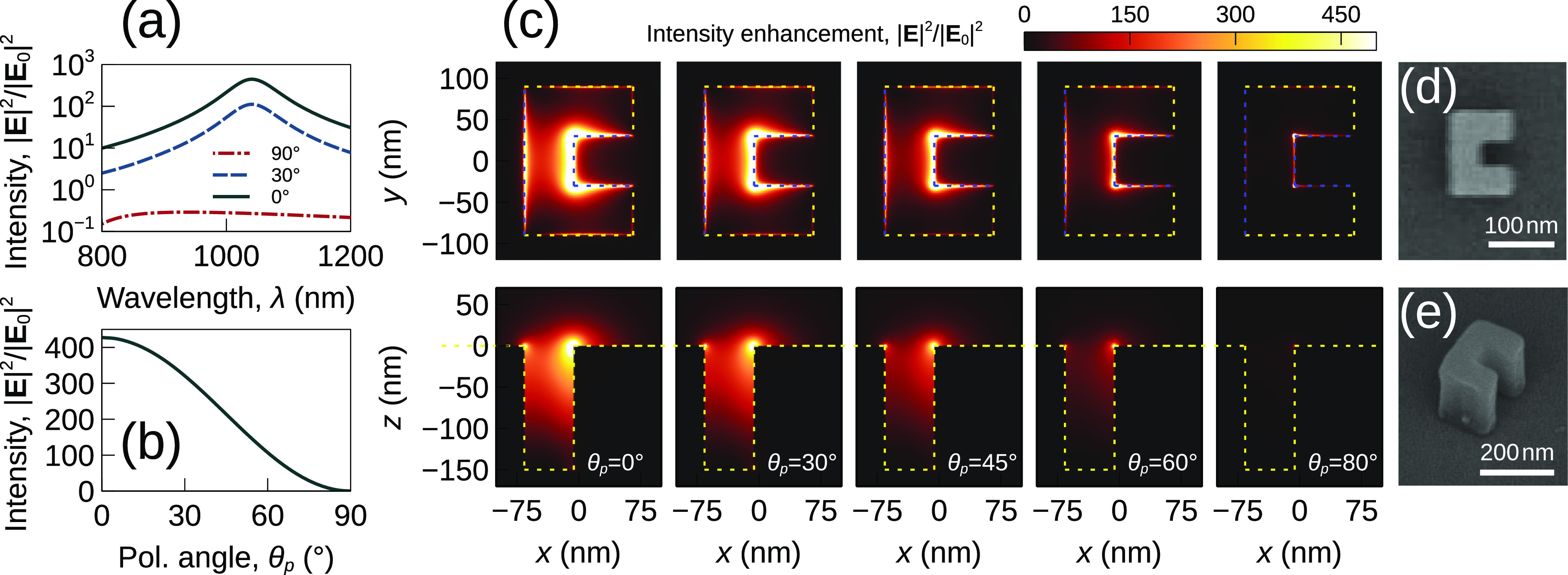
(a) Spectral response showing the intensity enhancement calculated at the point , (b) intensity enhancement as a function of the polarization angle, (c) xy and xz plane field intensity distributions around the CE at different polarization angles, and (d) and (e) SEM images of the fabricated C-structure (after photoresist patterning). The excitation wavelength is taken to be (near resonance wavelength) for (b) and (c). The plots at the top row and the bottom row in (c) share the same x axis. θp is measured with respect to the x axis. Input light intensity of is assumed for all simulations.
To quantify the force, the Maxwell stress tensor (MST)12,22,23 is used. The net force exerted on a particle can be calculated using the following MST formulation:
| (1) |
| (2) |
Here, is the Maxwell stress tensor, E is the electric field, H is the magnetic field, ϵw and μw are the permittivity and permeability of the surrounding medium (water), respectively, is the identity tensor, F is the net electromagnetic force exerted on the nanoparticle, S is the outer surface of the nanoparticle, and is the surface normal. The operator represents time-averaging. It should be noted that E and H depend on the particle position. Hence, mapping out the force profile requires recalculating the fields for different positions of the particle. The force profile calculated using this approach is shown in Fig. 3(a). For brevity, only the x component of the force (Fx) is plotted. A typical trapping force profile is observed with the equilibrium position located near x = 0. The corresponding potential distribution, ux, is shown in Fig. 3(b). A trapping potential well with depth greater than is observed, which is sufficient to overcome the thermal energy of a particle for stable trapping. Here, ux was obtained by integrating Fx along x.12,15 Note that this method assumes the force to be conservative (i.e., ). A more accurate estimation of the trapping potential can be obtained by using the Helmholtz–Hodge decomposition method,24 which works even if the force is non-conservative.
FIG. 3.
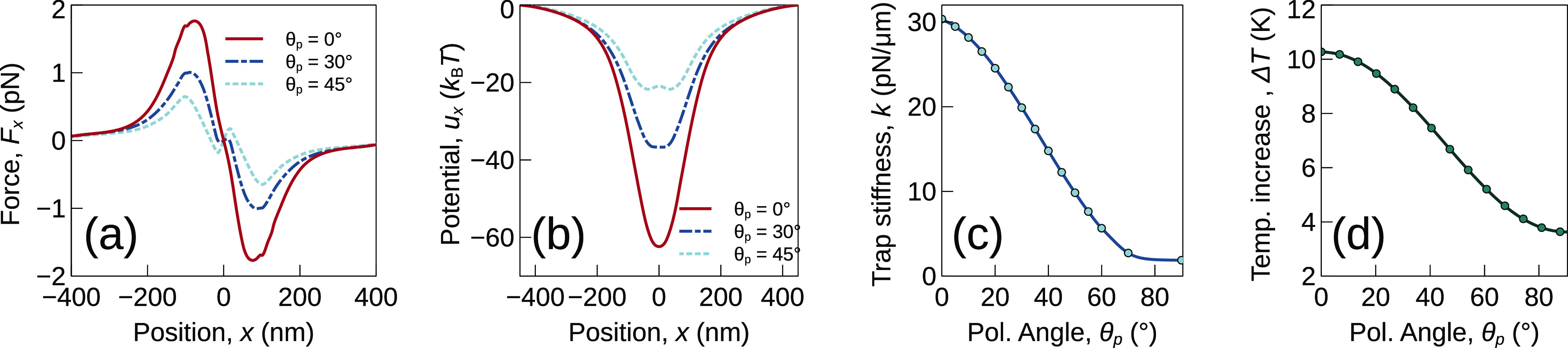
(a) Force profile along the x direction at y = 0, , (b) trapping potential corresponding to the force, (c) trap stiffness as a function of the polarization angle, and (d) temperature increase above ambient at the point (0, 0, 5 nm).
The parameter trap stiffness is often used to characterize optical traps.7,14 For small particle displacement around the equilibrium trap position, the optical force can be compared to the restoring force of a spring. The equivalent spring constant of this force is referred to as the trap stiffness, k. A stiffer trap implies tighter confinement of a trapped particle. We calculate k from the force and the potential using regression analysis (i.e., fitting data near the equilibrium position to the equations and ). The calculated stiffness as a function of the polarization angle is shown in Fig. 3(c). It is observed that the stiffness can be tuned over a large range ( ) by varying θp. The force value, potential well depth, and trap stiffness are largest for , which is consistent with our observation of the field distributions.
In addition to the force, the thermal characteristics are also important. The electromagnetic power losses in the materials convert to heat. The temperature increase due to this photo-thermal heating for different polarization angles is shown in Fig. 3(d). Details of the thermal analysis are discussed in the supplementary material. The results show that the configurations which produce larger fields have higher temperature increase. Thus, trapping with a lower field can reduce heating effects.
After obtaining the force distribution, the trajectory of a nanoparticle near the CE can be calculated from the Langevin equation.25,26 In a low Reynolds number environment (discussed in the supplementary material), the Langevin equation for a nanoparticle with negligible mass is given by
| (3) |
Here, is the particle position, F is the net external force acting on the particle, is the diffusion tensor, is the element-wise square root of , and is a vector white noise term, which models Brownian motion. In isotropic conditions, , where is the dynamic viscosity of water. Equation (3) is a stochastic differential equation that can be numerically solved using the Euler–Maruyama method27,28 to obtain sample trajectories. The solution approach discussed in Ref. 28 is used here. It should be noted that thermally induced fluid-flow may also affect particle trajectory, which is not taken into account in this model. According to Fig. 3(d), the maximum temperature increase is about 11 K at which the fluid velocity due to convection is not expected to be significant.29 This effect can be taken into account in a future work for a more comprehensive model.
Using the calculated force profile around the CE, nanoparticle trajectories for a few initial particle positions are studied. First, an initial position of is assumed which is about away from the trap center located at (0, 0). Figures 4(a) and 4(b) show the particle trajectory on the xy plane for and , respectively. The Brownian nature of the particle motion is easily discernible from plots. It can be observed that while the particle gets trapped for the case, this is not the case for . Figure 3(a) indicates that the peak force value is approximately four times less for . Hence, the nanoparticle at its initial position does not experience sufficient force for trapping. As a result, the trajectory is purely driven by the Brownian motion and appears random. However, when the initial position is selected closer to the trap at , trapping can be achieved even at as shown in Fig. 4(c). These simulations suggest that initially trapping a particle from a moderate distance may require a larger force, but it requires lesser force to confine the particle once it is near the trap. Since the field strength and the temperature experienced by a particle are significantly less for , as shown in Figs. 2(b) and 3(d), the particle would be exposed to less harsh conditions. It should also be noted that the high temperature region is located near the equilibrium trapping position only (discussed in the supplementary material). Thus, during the initial trapping phase with a high electric field, there should only be a brief time when the particle experiences a high temperature environment. Once trapped, the field is reduced which eliminates (or significantly decreases) the high-temperature region. Thus, when trapping sensitive bio-samples, a larger field can be used to draw a particle closer and then the field can be dynamically decreased to reduce thermal damage when it is already trapped.
FIG. 4.

Simulated trajectory of a nanoparticle for different initial positions (xi, yi) and polarization angles (θp).
To verify the design, the device is experimentally tested. The experimental parameters are kept identical to the simulation parameters. The details regarding the optical setup are provided in the supplementary material. During experiment, the motion of a trapped particle is recorded as the polarization angle is varied with the help of a half-wave plate. The captured video (multimedia file 1) is post-processed to extract particle position data. Any change in the trapping force would be reflected in the position data in the form of increased/decreased Brownian motion. Figure 5(a) shows the polarization angle at different times during the experiment, and Fig. 5(b) (Multimedia view) shows the corresponding particle position data along the x direction. A clear increase in Brownian motion can be observed when θp is increased from 0°. This clearly indicates that the trap stiffness and the potential well are being modulated by the polarization angle. To verify this further, numerical trajectory simulation data for the same θp sweep are shown in Fig. 5(c). The simulation and experimental results are in good agreement. Thus, a dynamically controllable plasmonic trap is achieved.
FIG. 5.

To summarize, CE based plasmonic tweezers with the ability to dynamically adjust the optical trapping force were presented. Experimental and numerical data show that the field distributions and the associated force profile can be varied by adjusting the polarization angle of the incident light. Using this mechanics, a trapped sample could be maintained in place with lower field values, which reduces the probability of thermal damage.
See the supplementary material for the details about the sample preparation, experimental setup, and thermal simulations.
Acknowledgments
This work was partially supported by the National Institutes of Health (NIH) via Grant No. R01GM138716. Part of this work was performed at the Stanford Nano Shared Facilities (SNSF), supported by the National Science Foundation (NSF) under Award No. ECCS-1542152.
AUTHOR DECLARATIONS
Conflict of Interest
The authors have no conflicts to disclose.
Author Contributions
Mohammad Asif Zaman: Conceptualization (equal); Formal analysis (equal); Investigation (equal); Methodology (equal); Software (equal); Visualization (equal); Writing – original draft (equal). Lambertus Hesselink: Conceptualization (equal); Funding acquisition (equal); Supervision (equal); Writing – review & editing (equal).
DATA AVAILABILITY
The data that support the findings of this study are available from the corresponding author upon reasonable request.
References
- 1. Ashkin A. and Dziedzic J., Science 235, 1517 (1987). 10.1126/science.3547653 [DOI] [PubMed] [Google Scholar]
- 2. Zhou J., Dai X., Jia B., Qu J., Ho H.-P., Gao B. Z., Shao Y., and Chen J., Appl. Phys. Lett. 120, 163701 (2022). 10.1063/5.0086855 [DOI] [Google Scholar]
- 3. Wang M. D., Yin H., Landick R., Gelles J., and Block S. M., Biophys. J. 72, 1335 (1997). 10.1016/S0006-3495(97)78780-0 [DOI] [PMC free article] [PubMed] [Google Scholar]
- 4. Tan H., Hu H., Huang L., and Qian K., Analyst 145, 5699 (2020). 10.1039/D0AN00577K [DOI] [PubMed] [Google Scholar]
- 5. Wright W., Sonek G., and Berns M., Appl. Phys. Lett. 63, 715 (1993). 10.1063/1.109937 [DOI] [Google Scholar]
- 6. Juan M. L., Righini M., and Quidant R., Nat. Photonics 5, 349 (2011). 10.1038/nphoton.2011.56 [DOI] [Google Scholar]
- 7. Kotsifaki D. G., Truong V. G., and Chormaic S. N., Appl. Phys. Lett. 118, 021107 (2021). 10.1063/5.0032846 [DOI] [Google Scholar]
- 8. Wang K., Schonbrun E., Steinvurzel P., and Crozier K. B., Nat. Commun. 2, 469 (2011). 10.1038/ncomms1480 [DOI] [PubMed] [Google Scholar]
- 9. Kwak E.-S., Onuta T.-D., Amarie D., Potyrailo R., Stein B., Jacobson S. C., Schaich W., and Dragnea B., J. Phys. Chem. B 108, 13607 (2004). 10.1021/jp048028a [DOI] [Google Scholar]
- 10. Wong H. M. K., Righini M., Gates J. C., Smith P. G. R., Pruneri V., and Quidant R., Appl. Phys. Lett. 99, 061107 (2011). 10.1063/1.3625936 [DOI] [Google Scholar]
- 11. Zhang Y., Min C., Dou X., Wang X., Urbach H. P., Somekh M. G., and Yuan X., Light 10, 59 (2021). 10.1038/s41377-021-00474-0 [DOI] [PMC free article] [PubMed] [Google Scholar]
- 12. Ren Y., Chen Q., He M., Zhang X., Qi H., and Yan Y., ACS Nano 15, 6105 (2021). 10.1021/acsnano.1c00466 [DOI] [PubMed] [Google Scholar]
- 13. Shi X. and Hesselink L., J. Opt. Soc. Am., B 21, 1305 (2004). 10.1364/JOSAB.21.001305 [DOI] [Google Scholar]
- 14. Neuman K. C. and Block S. M., Rev. Sci. Instrum. 75, 2787 (2004). 10.1063/1.1785844 [DOI] [PMC free article] [PubMed] [Google Scholar]
- 15. Kotsifaki D. G. and Chormaic S. N., Nanophotonics 8, 1227 (2019). 10.1515/nanoph-2019-0151 [DOI] [Google Scholar]
- 16. Righini M., Volpe G., Girard C., Petrov D., and Quidant R., Phys. Rev. Lett. 100, 186804 (2008). 10.1103/PhysRevLett.100.186804 [DOI] [PubMed] [Google Scholar]
- 17. Zaman M. A., Padhy P., and Hesselink L., Phys. Rev. A 96, 043825 (2017). 10.1103/PhysRevA.96.043825 [DOI] [Google Scholar]
- 18. Ndukaife J. C., Kildishev A. V., Nnanna A. G. A., Shalaev V. M., Wereley S. T., and Boltasseva A., Nat. Nanotechnol. 11, 53 (2016). 10.1038/nnano.2015.248 [DOI] [PubMed] [Google Scholar]
- 19. Zheng Y., Ryan J., Hansen P., Cheng Y.-T., Lu T.-J., and Hesselink L., Nano Lett. 14, 2971 (2014). 10.1021/nl404045n [DOI] [PubMed] [Google Scholar]
- 20. Matteo J., Fromm D., Yuen Y., Schuck P., Moerner W., and Hesselink L., Appl. Phys. Lett. 85, 648 (2004). 10.1063/1.1774270 [DOI] [Google Scholar]
- 21. Johnson P. B. and Christy R.-W., Phys. Rev. B 6, 4370 (1972). 10.1103/PhysRevB.6.4370 [DOI] [Google Scholar]
- 22. Yannopapas V., Phys. Rev. B 78, 045412 (2008). 10.1103/PhysRevB.78.045412 [DOI] [Google Scholar]
- 23. Miljkovic V. D., Pakizeh T., Sepulveda B., Johansson P., and Kall M., J. Phys. Chem. C 114, 7472 (2010). 10.1021/jp911371r [DOI] [Google Scholar]
- 24. Zaman M. A., Padhy P., Hansen P. C., and Hesselink L., Appl. Phys. Lett. 112, 091103 (2018). 10.1063/1.5016810 [DOI] [Google Scholar]
- 25. Volpe G. and Volpe G., Am. J. Phys. 81, 224 (2013). 10.1119/1.4772632 [DOI] [Google Scholar]
- 26. Lukić B., Jeney S., Sviben Ž., Kulik A. J., Florin E.-L., and Forró L., Phys. Rev. E 76, 011112 (2007). 10.1103/PhysRevE.76.011112 [DOI] [PubMed] [Google Scholar]
- 27. Higham D. J., SIAM Rev. 43, 525 (2001). 10.1137/S0036144500378302 [DOI] [Google Scholar]
- 28. Zaman M. A., Wu M., Padhy P., Jensen M. A., Hesselink L., and Davis R. W., Micromachines 12, 1265 (2021). 10.3390/mi12101265 [DOI] [PMC free article] [PubMed] [Google Scholar]
- 29. Roxworthy B. J., Bhuiya A. M., Vanka S. P., and Toussaint K. C., Nat. Commun. 5, 3173 (2014). 10.1038/ncomms4173 [DOI] [PubMed] [Google Scholar]
Associated Data
This section collects any data citations, data availability statements, or supplementary materials included in this article.
Supplementary Materials
See the supplementary material for the details about the sample preparation, experimental setup, and thermal simulations.
Data Availability Statement
The data that support the findings of this study are available from the corresponding author upon reasonable request.