The numerical solution of a mathematical model of the Covid-19 pandemic utilizing a meshless local discrete Galerkin method

Abstract

It was in early December 2019 that the terrible news of the outbreak of new coronavirus disease (Covid-19) was reported by the world media, which appeared in Wuhan, China, and is rapidly spreading to other parts of China and several overseas countries. In the field of infectious diseases, modeling, evaluating, and predicting the rate of disease transmission are very important for epidemic prevention and control. Several preliminary mathematical models for Covid-19 are formulated by various international study groups. In this article, the SEIHR(D) compartmental model is proposed to study this epidemic and the factors affecting it, including vaccination. The proposed model can be used to compute the trajectory of the spread of the disease in different countries. Most importantly, it can be used to predict the impact of different inhibition strategies on the development of Covid-19. A computational approach is applied to solve the offered model utilizing the Galerkin method based on the moving least squares approximation constructed on a set of scattered points as a locally weighted least square polynomial fitting. As the method does not need any background meshes, its algorithm can be easily implemented on computers. Finally, illustrative examples clearly show the reliability and efficiency of the new technique and the obtained results are in good agreement with the known facts about the Covid-19 pandemic.

Introduction

Coronaviruses are RNA single-stranded positive viruses about 26–32 kilobytes in size and covered with symmetrical polyhedral particles approximately 80–200 nm in diameter. These types of viruses have a wide range of hosts, including birds and wild animals, infect wild and domestic mammals, which can be infected humans through animal agents [15, 54]. Most human coronaviruses usually cause relatively mild respiratory illness [25]. The coronavirus family is divided into four genera: $\alpha ,\beta ,\gamma ,\delta$-Cov. The $\alpha ,\beta$-Cov can infect mammals, while $\gamma ,\delta$-Cov tend to infect birds [28]. Six species of human viruses have been reported since the 1960s. Four of them (229E and NL63 of type $\alpha$ and HKU1 and OC43 of type $\beta$) cause mild illnesses such as colds and gastrointestinal infections [56]. However, two types of coronaviruses, SARS-Cov and MERS-Cov, may cause severe illness and eventually death [58].

The SARS virus, thought to be spread by bats in China, created a global SARS epidemic in 2002 that killed about 800 people. Coronavirus SARS causes acute and severe respiratory syndrome in patients [46]. The outbreak of the coronavirus Mers in 2012, known as Middle East Respiratory Syndrome, killed 858 people in the Middle East. A new coronavirus has been identified to cause respiratory illness, such as atypical pneumonia, in humans. This disease, with the interim name “2019-nCov acute respiratory disease (ARD)” (official name: Covid-19), is first detected in the winter month of December 2019 in Wuhan city with a population of 11 million people in Hubei Province, China. The 2019-nCov is believed to be zoonotic in origin, from bats to intermediate hosts to humans, and its initiation is geographically associated, but with uncertainty, with the Huanan Seafood Market in Wuhan.

Covid-19 features mild symptoms in most cases, and short serial intervals [40, 60] are similar to the pandemic in influenza, rather than other coronaviruses. Therefore, it may be reasonable to look for the 1918 modeling framework in the influenza epidemic history in London, United Kingdom [29]. To model the spread of a disease in a population, a very logical choice is to use compartmental models. In such models, the population is divided into compartments that show the progression of the disease. To better understand the dynamics of Covid-19, researchers have proposed several models. A mathematical model incorporating the presence of undetected infectious cases, sanitizing conditions of hospitalized cases, and the fraction of detected cases was proposed in [31]. Yang and Wang [59] gave an SEIR model which incorporating environment-to-human and human-to-human transmission routes. The effect of delay in diagnosis on disease transmission with a deterministic model is investigated in [42]. The authors reported that increasing the proportion of timely diagnosis is not sufficient for the eradication of Covid-19 but can effectively reduce the transmission risk.

The compartment models based on partial differential equations (PDEs) are significantly less common than conventional ordinary differential equation (ODE) models, especially due to the increased hardness and time involved in execution and numerical solution. However, such additional costs are offset by the fact that PDE models naturally store spatial information, which makes it possible to continuously describe spatio-temporal dynamics with the potential for geographical features, population heterogeneity, and multidimensional dynamics. In fact, recent research shows that the release of Covid-19 offers multidisciplinary characteristics ranging from the scale of the virus and the individual immune system to the collective behavior of the entire population [6]. For the scale of virus transmission between individuals, there are studies such as the area of potential infection produced by cough [64] or the spread of the virus in a built environment [39]. On a smaller scale, the anti-viral effects can even be studied with ultraviolet light [63]. The space–time-dependent model of Covid-19 has been solved [9, 24, 51].

In recent years, the main focus of the applications of meshless methods seems to have shifted from scattered data approximation to computational mathematics [12, 13]. The most usual basic meshfree methods are known in the literature as radial basis functions (RBFs) and the moving least squares (MLS) methods. The MLS scheme, as a general case of Shepard’s method, has been introduced by Lancaster and Salkauskas [32]. The MLS consists of a local weighted least squares fitting, valid on a small neighborhood of a point and only based on the information provided by its closest points. The MLS algorithm involves a single independent variable weight function regardless of the dimension of the problem, so applying them in higher dimensions is simple. A valuable advantage of using the MLS approximation is that it sets up and solves many small systems, instead of a single, but large system [17, 55].

We would like to review some applications of meshless methods in various problems of computational mathematics. The Galerkin boundary node method [37, 38] has been utilized for two-dimensional exterior Neumann problems. Element-free Galerkin methods [7] have been given to solve the elasticity and heat conduction problems. The local boundary integral equation method [45] has been applied to solve the problem of elasticity. The RBF method [10] has been developed for solving coupled Burgers’ equations [43], hyperbolic PDEs [44], the heat conduction equation [19, 22], nonhomogeneous elastic problems [23], inverse wave propagation problems [53] fracture mechanics equations [52] and hyperbolic conservation laws [26, 27]. The meshless discrete collocation schemes have been investigated for solving two-dimensional weakly singular integral equations [3, 4]. Authors of [20, 21] have investigated a domain-type RBF collocation method to solve special integro-differential models as fractional diffusion models. The reproducing kernel method has been applied for solving integro-differential equations [1, 2], an MLS-based Galerkin meshless method [5, 36] has been utilized to solve logarithmic boundary integral equations.

In the current work, we present a time-dependent SEIHR(D) compartmental model for Covid-19 disease, including a system of ODEs. The effect of vaccination is also investigated in this model by adding a new compartment. This article gives a computational scheme based on the MLS method for solving the presented mathematical model for Covid-19. To start the method, we first reduce the system of ODEs derived from SEIHR(D) model to equivalent to a system of Volterra integral equations. Subsequently, the solution of the mentioned system of Volterra integral equations is estimated by the discrete Galerkin method together with the shape functions of the MLS constructed on a set of nodal points as a basis. The numerical scheme developed in the current paper utilizes the non-uniform Gauss–Legendre quadrature rule to estimate all integrals in the method. We are also interested in studying the dynamics of viruses spread in specific areas by a system of PDEs. Therefore, we extend the proposed scheme to a space–time-dependent SEIHR(D) model for Covid-19 on two-dimensional space domains. Traditional numerical methods to solve PDE problems of this type in space dimensions $\ge 2$, such as the finite element method, use an underlying mesh (e.g., a triangulation) for the definition of basis functions or elements [18]. Developing and reconstructing a mesh often represent a significant hurdle to accomplish these methods. Since the offered scheme does not require any mesh generations on the domain, it is free from these difficulties.

In the following, we consider the outline of the article. In Sect. 2, we propose a compartmental model for Covid-19 disease. In Sect. 3 reviews some of the basic formulations and properties of the MLS approximation. In Sect. 4, we present a numerical method for solving the time and space–time-dependent SEIHR(D)-compartment model based on the MLS approximation and the Gauss–Legendre formula in the Galerkin method. We consider illustrated examples in Sect. 5. Finally, the conclusion of the paper is given in Sect. 6.

Covid-19 mathematical model

When we use a mathematical model to discuss the dynamics of the progression and transmission of a particular disease in a community, it can be used to consider different ways to control this disease. Although social, political and economic factors have a special role in planning the health principles of a society, the use of mathematical models has a very important role in decision making. As one of the first academic works in the field of mathematical models of diseases, Daniel Bernoulli and Jean Le Rond d’Alembert argued for a smallpox vaccination model in the late 1700s [8, 14]. In 1927, Kermack and McKendrick proposed a simple mathematical model to study the dynamics of the spread of infectious diseases [47]. In this model, the people who live in a community are divided into three groups which are known as the SIR model.

To model the Covid-19 pandemic, we consider six compartments for people in a community as follows. Susceptible, indicated by S, includes those who are healthy and can get a disease. Exposed, indicated by E, includes those who are infected and can transmit the disease, but they have not been identified as patients yet by a standard test for Covid-19. Infective, indicated by I, includes those who are infected whose test results are positive for the disease and can also transmit the disease. Hospitalized, indicated by H, includes those who are hospitalized. Recovered, indicated by R, includes people who have recovered from the disease and are immune to it. Deaths, indicated by D, include those who are dead. The progression of the disease is shown schematically in Fig. 1. Based on the clinical progression of the disease, epidemiological status of the individuals and intervention measures (including government measures, segregation, protection, etc.), we propose a deterministic Covid-19 transmission model.

Fig. 1.

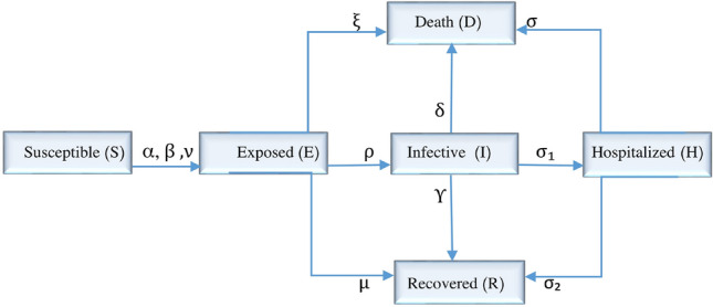
The proposed compartmental epidemic model

Let N(t) denote the sum of the total population, i.e.,

$$\begin{array}{c}\hfill N(t)=S(t)+E(t)+I(t)+H(t)+R(t).\end{array}$$

The population of susceptible individuals in group S is decreased by the exposed individuals in group E (at the rate $\alpha (t)$), infective individuals in group I (at a rate $\beta (t)$) and hospitalized individuals in group H (at the rate $\nu$), so that

$$\begin{array}{c}\hfill \frac{\text{d}S(t)}{\text{d}t}=-\left(\alpha ,(,t,),E,(,t,),+,\beta ,(,t,),I,(,t,),+,\nu ,H,(,t,)\right)\frac{S(t)}{N(t)},\end{array}$$ 1

the initial population of these people is $S(0)=s_0$.

It should be noted that the parameters $\alpha (t)$, $\beta (t)$ and $\nu$ are the average number of contacts per person per time, multiplied by the probability of disease transmission in contact between a susceptible with an exposed, an infectious and a hospitalized, respectively. $\alpha (t)$ usually has a downward trend over time, the amount of which depends generally on public awareness, government measures, quarantine, medical facilities and health principles. $\beta (t)$ also depends on similar factors in some way, especially how to quarantine of infectious people. So, it can be considered as a descending function in terms of time. Since infectious people after diagnosis generally have to be in home quarantine and, therefore, their number of contacts with other people is limited, $\beta (t)$ is chosen smaller with less changes over time compared to $\alpha (t)$. As people who are admitted to the hospital are only in contact with the treatment staff, $\nu$ is selected a small fixed number.

The population of exposed individuals in group E is generated by susceptible individuals in group S and decreases as the disease progresses, recovery and death in group E (at the rates $\rho (t)$, $\mu$ and $\xi$). Hence,

$$\begin{array}{c}\hfill \frac{\text{d}E(t)}{\text{d}t}=\left(\alpha ,(,t,),E,(,t,),+,\beta ,(,t,),I,(,t,),+,\nu ,H,(,t,)\right)\frac{S(t)}{N(t)}-\rho (t)E(t)-\left(\mu ,+,\xi \right)E(t),\end{array}$$ 2

where the initial population of this group is $E(0)=e_0$.

The rate $\rho (t)$ as a diagnostic parameter can be considered as ascending function respect to time, because the diagnostic parameter increases during the course of the disease due to the advancement of facilities, such as laboratory kits. So that by increasing $\rho (t)$ and quarantining known patients, this parameter has a significant impact on the prevalence and control of Covid-19.

The population of infective individuals in group I is generated by the disease progresses in group E (at a rate $\rho$). It is decreased by recovery, death in group I (at the rates $\gamma$ and $\delta$) and with the progression of the disease in this group and its transfer to the group H (at a rate ${\sigma }_1$), so

$$\begin{array}{c}\hfill \frac{\text{d}I(t)}{\text{d}t}=\rho (t)E(t)-\left(\gamma ,+,\delta \right)I(t)-{\sigma }_{1}I(t),\end{array}$$ 3

the initial population of this group is $I(0)=i_0$.

The population of hospitalized individuals in group H is generated by the disease progresses in group I (at a rate ${\sigma }_1$) and decreased by recovery and death in this group (at the rates ${\sigma }_2$ and $\sigma$). Thus,

$$\begin{array}{c}\hfill \frac{\text{d}H(t)}{\text{d}t}={\sigma }_{1}I(t)-\left({\sigma }_2,+,\sigma \right)H(t),\end{array}$$ 4

and has an initial population of $H(0)=h_0$.

Based on the above assumptions, the device of differential equations governing the proposed model is obtained as follows:

$$\begin{array}{c}\hfill \left\{\begin{array}{cc}\frac{\text{d}S(t)}{\text{d}t}=-\left(\alpha ,(,t,),E,(,t,),+,\beta ,(,t,),I,(,t,),+,\nu ,H,(,t,)\right)\frac{S(t)}{N(t)},\hfill & \hfill \\ \hfill \\ \frac{\text{d}E(t)}{\text{d}t}=\left(\alpha ,(,t,),E,(,t,),+,\beta ,(,t,),I,(,t,),+,\nu ,H,(,t,)\right)\frac{S(t)}{N(t)}-\rho (t)E(t)-\left(\mu ,+,\xi \right)E(t),\hfill & \hfill \\ \hfill \\ \frac{\text{d}I(t)}{\text{d}t}=\rho (t)E(t)-\left(\gamma ,+,\delta \right)I(t)-{\sigma }_{1}I(t),\hfill & \hfill \\ \hfill \\ \frac{\text{d}H(t)}{\text{d}t}={\sigma }_{1}I(t)-\left({\sigma }_2,+,\sigma \right)H(t),\hfill & \hfill \end{array}\right)\end{array}$$ 5

with initial conditions

$$\begin{array}{c}\hfill S(0)=s_0,E(0)=e_0,I(0)=i_0\text{and}H(0)=h_0.\end{array}$$

Since births and natural deaths are not considered during this disease period, N(t) is equal to the initial population, i.e., $N_0$, regardless of time.

The population of recovered individuals in group R is generated by the recovery in group E (at a rate $\mu$), recovery in group I (at a rate $\gamma$) and recovered individuals in group H (at a rate ${\sigma }_2$), so that

$$\begin{array}{c}\hfill \frac{\text{d}R(t)}{\text{d}t}=\mu E(t)+\gamma I(t)+{\sigma }_{2}H(t).\end{array}$$ 6

The initial population recovered from the disease is $R(0)=r_0$.

The population of deceased individuals in group D is generated by death in group E (at a rate $\xi$), death in group I (at a rate $\delta$) and deceased individuals in group H (at a rate $\sigma$). Thus,

$$\begin{array}{c}\hfill \frac{\text{d}D(t)}{\text{d}t}=\xi E(t)+\delta I(t)+\sigma H(t),\end{array}$$ 7

where $D(0)=d_0$ is the number of people who died at the initial time.

Therefore, the number of people who have recovered and died of the disease can be obtained from the following device:

$$\begin{array}{c}\hfill \left\{\begin{array}{cc}\frac{\text{d}R(t)}{\text{d}t}=\mu E(t)+\gamma I(t)+{\sigma }_{2}H(t),\hfill & \hfill \\ \hfill \\ \frac{\text{d}D(t)}{\text{d}t}=\xi E(t)+\delta I(t)+\sigma H(t),\hfill & \hfill \end{array}\right)\end{array}$$ 8

with the conditions

$$\begin{array}{c}\hfill R(0)=r_0\text{and}D(0)=d_0.\end{array}$$

The parameters of the model are listed in Table 1 and the unit of all the parameters is ${\text{day}}^{-1}$.

Table 1.

The parameters of the SEIHR(D) model

Symbol	Interpretation
$\alpha (t)$	The transmission rate of disease from exposed individuals at the time t
$\beta (t)$	The transmission rate of disease from infective individuals at the time t
$\nu$	The transmission rate of disease from hospitalized individuals
$\rho (t)$	Rate of disease progression of exposed individuals at the time t
$\xi$	The death rate of exposed individuals
$\mu$	The recovery rate of exposed individuals
$\gamma$	The recovery rate of infective individuals
$\delta$	The death rate of infective individuals
${\sigma }_1$	Rate of disease progression of infective individuals
${\sigma }_2$	The recovery rate of hospitalized individuals
$\sigma$	The death rate of hospitalized individuals

Remark 1

Here the question arises, can an infectious disease attack a population that is in a static population situation with all susceptible individuals? To answer this question, the reproduction number is mathematically defined as the expected secondary number produced by a typical infected individual during its entire infectious period in a susceptible population. Explaining of the time course of an epidemic can be partly achieved by estimating the effective reproduction number $R_t$ defined as the actual average number of secondary cases per primary case at calendar time $t>0$, which is given for a certain susceptible population fraction S/N by [16]

$$\begin{array}{c}\hfill R_t=\left(\frac{\alpha }{\rho +\mu +\xi },+,\frac{\beta \rho }{(\rho +\mu +\xi )(\gamma +\delta +{\sigma }_1)},+,\frac{\nu \rho {\sigma }_1}{(\rho +\mu +\xi )(\gamma +\delta +{\sigma }_1)(\sigma +{\sigma }_2)}\right)\frac{S}{N}.\end{array}$$ 9

Note that $R_t$ shows time-dependent variation due to the decline in susceptible individuals (intrinsic factors) and the implementation of control measures (extrinsic factors). If $R_t\le 1$, it suggests that the epidemic is in decline and may be regarded as being under control at time t and conversely this situation occurs when $R_t>1$. The basic reproduction number $R_0$ is considered by evaluating at the trivial disease-free equilibrium ($S=1$ and $E,I,H,R,D=0$), i.e.,

$$\begin{array}{c}\hfill R_0=\left(\frac{\alpha }{\rho +\mu +\xi },+,\frac{\beta \rho }{(\rho +\mu +\xi )(\gamma +\delta +{\sigma }_1)},+,\frac{\nu \rho {\sigma }_1}{(\rho +\mu +\xi )(\gamma +\delta +{\sigma }_1)(\sigma +{\sigma }_2)}\right).\end{array}$$ 10

Indeed, the quantity $R_0$ must be bigger than 1 to occur an epidemic in a susceptible population.

The basic reproductive number is affected by several factors, such as [34]:

• $✓$ The rate of contact in the host population.

• $✓$ The probability of infection being transmitted during contact.

• $✓$ The duration of infectiousness.

Derivation and discussion of the basic reproduction number make evaluating the effectiveness of different containment measures more clear, as the dependence of transmission in terms of the model parameters becomes explicit (for more details, see [11, 16])

Vaccination effect on the model

Vaccines to prevent Covid-19 infection are considered the most promising approach for curbing the Covid-19 pandemic. All vaccine platforms are designed to train our immune system. Currently, there are several Covid-19 vaccines available around the world, which are generally divided into four categories including inactivated virus vaccine, viral vector vaccine, encapsulated mRNA vaccine and recombinant protein vaccine. The World Health Organization (WHO) maintains an updated list of vaccine candidates under evaluation [62]. All vaccines approved by WHO are highly effective, substantially reduce the risk of Covid-19, especially severe diseases, and have been associated with substantial reductions in Covid-19-associated hospitalizations and deaths [48–50]. In addition to direct reductions in Covid-19-associated morbidity and mortality, vaccination has been associated with lower non-Covid-19 mortality rates, supporting evidence that Covid-19 vaccination does not increase the risk of death [57].

To observe the effect of the vaccination on the Covid-19 pandemic, especially the infected people, we add the vaccination compartment to the previous model and apply the necessary changes to the dynamic system. The schematic of the model is drawn in Fig. 2. Let susceptible people be vaccinated at the rate $v_1$, so its effect on the equation (1) can be considered as follows:

$$\begin{array}{c}\hfill \frac{\text{d}S(t)}{\text{d}t}=-\left(\alpha ,(,t,),E,(,t,),+,\beta ,(,t,),I,(,t,),+,\nu ,H,(,t,)\right)\frac{S(t)}{N(t)}-v_{1}S(t).\end{array}$$ 11

On the other hand, we assume that the used vaccine has an inefficacy rate $v_2$ and an efficacy rate $v_3$. Therefore, vaccinated people with the rates $v_2\alpha (t)$, $v_2\beta (t)$ and $v_2\nu$ may be re-infected in contact with exposed individuals, infected individuals and hospitalized individuals and enter the compartment of exposed people, and also the vaccinated people with the rate $v_3$ recover and become immune. Susceptible people who receive the vaccine enter the compartment of the vaccinated. The differential equation describing the compartment of vaccinated people is given as

$$\begin{array}{c}\hfill \frac{\text{d}V(t)}{\text{d}t}=v_{1}S(t)-v_2\left(\alpha ,(,t,),E,(,t,),+,\beta ,(,t,),I,(,t,),+,\nu ,H,(,t,)\right)\frac{V(t)}{N(t)}-v_{3}V(t),\end{array}$$ 12

with the initial condition $V(0)=v_0$. For the differential equations describing recovered and exposed people, we have the following changes

$$\begin{array}{cc}\hfill \frac{\text{d}E(t)}{\text{d}t}& =\left(\alpha ,(,t,),E,(,t,),+,\beta ,(,t,),I,(,t,),+,\nu ,H,(,t,)\right)\frac{S(t)}{N(t)}-\rho (t)E(t)\hfill \\ \hfill & -\left(\mu ,+,\xi \right)E(t)+v_2\left(\alpha ,(,t,),E,(,t,),+,\beta ,(,t,),I,(,t,),+,\nu ,H,(,t,)\right)\frac{V(t)}{N(t)},\hfill \end{array}$$ 13

and

$$\begin{array}{c}\hfill \frac{\text{d}R(t)}{\text{d}t}=\mu E(t)+\gamma I(t)+{\sigma }_{2}H(t)+v_{3}V(t).\end{array}$$ 14

Fig. 2.

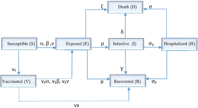
The proposed compartmental epidemic model with vaccination effect

Space–time model for Covid-19

We investigate the SEIHR(D) model when the effect of the space is also considered on the spread of the disease. This model enables the continuous description of spatio-temporal dynamics with the potential of geographic features, population heterogeneity and multidimensional dynamics. In fact, this model states that the movement of people in each compartment affects the progression of the disease. Let $\mathrm{\Omega }\subset {\mathbb{R}}^2$ be a two-dimensional simply connected domain with the boundary $\partial \mathrm{\Omega }$ and $[0,t_f]$ denote a generic time interval. Therefore, by making the functions dependent on space as well as time, the following system of coupled PDEs over $\mathrm{\Omega }\times [0,t_f]$ is given to simulate a space–time model for Covid-19:

$$\begin{array}{c}\hfill \left\{\begin{array}{cc}\frac{\partial \mathbf{u}(t,\mathbf{x})}{\partial t}=\left(\mathbf{A},+,\mathbf{B},\left(\mathbf{u},(,t,,,\mathbf{x},)\right)\right)\mathbf{u}(t,\mathbf{x})+\mathrm{\nabla }·\left(\mathbf{v},\mathrm{\nabla },\mathbf{u},(,t,,,\mathbf{x},)\right),\hfill & (t,\mathbf{x})\in [0,t_f]\times \mathrm{\Omega },\hfill \\ \hfill \\ \mathbf{v}\mathrm{\nabla }\mathbf{u}(t,\mathbf{x})·n=\mathbf{g}(t,\mathbf{x}),\hfill & (t,\mathbf{x})\in [0,t_f]\times \partial \mathrm{\Omega },\hfill \\ \hfill \\ \mathbf{u}(0,\mathbf{x})={\mathbf{u}}_0(\mathbf{x}),\hfill & \mathbf{x}\in \mathrm{\Omega },\hfill \end{array}\right)\end{array}$$ 15

where $\mathbf{u}(t,\mathbf{x})$ is the compact vector notation to represent the compartments as follows:

$$\begin{array}{c}\hfill \mathbf{u}(t,\mathbf{x})={\left[S,(,t,,,\mathbf{x},),,,E,(,t,,,\mathbf{x},),,,I,(,t,,,\mathbf{x},),,,H,(,t,,,\mathbf{x},),,,R,(,t,,,\mathbf{x},),,,D,(,t,,,\mathbf{x},)\right]}^T,\end{array}$$

where the unknown functions depend on both the time t and the space $\mathbf{x}$. The given function $\mathbf{g}$ is specified values on the Neumann condition on the boundary $\partial \mathrm{\Omega }$ and $\text{n}$ is the unit outward vector to $\partial \mathrm{\Omega }$. The tensors $\mathbf{A}$, $\mathbf{B}$ and $\mathbf{v}$ are defined according to the particular dynamics of the system, i.e.,

$$\begin{array}{cc}\hfill \mathbf{A}=& \left[\begin{array}{cccccc}0& 0& 0& 0& 0& 0\\ 0& -\rho (t,\mathbf{x})-\mu -\xi & 0& 0& 0& 0\\ 0& \rho (t,\mathbf{x})& -\gamma -\delta -{\sigma }_1& 0& 0& 0\\ 0& 0& {\sigma }_1& -{\sigma }_2-\sigma & 0& 0\\ 0& \mu & \gamma & {\sigma }_2& 0& 0\\ 0& \xi & \delta & \sigma & 0& 0\end{array}\right],\hfill \end{array}$$ 16

$$\begin{array}{cc}\hfill \mathbf{B}=& \left[\begin{array}{cccccc}0& -\alpha (t,\mathbf{x})S& -\beta (t,\mathbf{x})S& -\nu S& 0& 0\\ 0& \alpha (t,\mathbf{x})S& \beta (t,\mathbf{x})S& \nu S& 0& 0\\ 0& 0& 0& 0& 0& 0\\ 0& 0& 0& 0& 0& 0\\ 0& 0& 0& 0& 0& 0\\ 0& 0& 0& 0& 0& 0\end{array}\right],\hfill \end{array}$$ 17

and

$$\begin{array}{c}\hfill \mathbf{v}=\left[\begin{array}{cccccc}{\mathbf{v}}_S& 0& 0& 0& 0& 0\\ 0& {\mathbf{v}}_E& 0& 0& 0& 0\\ 0& 0& {\mathbf{v}}_I& 0& 0& 0\\ 0& 0& 0& {\mathbf{v}}_H& 0& 0\\ 0& 0& 0& 0& {\mathbf{v}}_R& 0\\ 0& 0& 0& 0& 0& 0\end{array}\right],\end{array}$$ 18

where

$$\begin{array}{c}\hfill {\mathbf{v}}_j=\left[\begin{array}{cc}{v}_{\mathit{xx}}^j& v_{\mathit{xy}}^j\\ v_{\mathit{yx}}^i& v_{\mathit{yy}}^i\end{array}\right],j=S,E,I,H,R.\end{array}$$ 19

In most applications, $\mathbf{v}=\mathbf{v}(t,\mathbf{x})$, i.e., diffusion is time dependent, heterogeneous, and anisotropic. In addition, we consider the following homogeneous Neumann boundary conditions:

$$\begin{array}{c}\hfill (\mathbf{v}\mathrm{\nabla }\mathbf{u})·n=0.\end{array}$$ 20

The MLS approximation

Given data values of the function $u(\mathbf{x})$ at certain data sites $X=\{{\mathbf{x}}_1,\dots ,{\mathbf{x}}_N\}$ in the closed domain $\mathrm{\Omega }\subset {\mathbb{R}}^d$. The idea of the MLS method is to approximate $u(\mathbf{x})$ for every point $\mathbf{x}\in \mathrm{\Omega }$ in a weighted least squares sense. For $\mathbf{x}\in \mathrm{\Omega }\subset {\mathbb{R}}^d$, the value $s_{u,X}(\mathbf{x})$ of the MLS approximation is given by the solution of

$$\begin{array}{c}\hfill min\left\{\sum _{i=1}^N,{[u({\mathbf{x}}_i)-p({\mathbf{x}}_i)]}^2,w,(\mathbf{x},{\mathbf{x}}_i),:,p,\in ,{\mathrm{\Pi }}_q,({\mathbb{R}}^d)\right\},\end{array}$$ 21

where $w:\mathrm{\Omega }\times \mathrm{\Omega }\to [0,\infty ]$ is a continuous weight function and ${\mathrm{\Pi }}_q({\mathbb{R}}^d)$ is the linear space of polynomials of total degree less than or equal to q in d-variables with the basis $\{p_1,\dots ,p_J\}$ [55]. We are mainly interested in the local continuous weight function w, which gets smaller as its arguments move away from each other. Ideally, w vanishes for arguments $\mathbf{x},\mathbf{y}\in \mathrm{\Omega }$ with ${\Vert \mathbf{x}-\mathbf{y}\Vert }_2$ greater than a certain threshold. Therefore, we can assume that

$$\begin{array}{c}\hfill w(\mathbf{x},\mathbf{y})={\mathrm{\Phi }}_{\delta }(\mathbf{x}-\mathbf{y})=\varphi \left(\frac{{\Vert \mathbf{x}-\mathbf{y}\Vert }_2}{\delta }\right),\delta >0,\end{array}$$ 22

where $\mathrm{\Phi }$ is a radial function, meaning that $\mathrm{\Phi }(\mathbf{x})={\varphi (\Vert \mathbf{x}\Vert }_2),\mathbf{x}\in {\mathbb{R}}^d$, in which $\varphi$ is a univariate and non-negative function, $\varphi :[0,\infty )\to \mathbb{R}$, with the property $\varphi (r)=0$ when $r\ge 1$ [55].

In the following theorem, we will find a direct approach to obtain the solution of the problem (21), but prior to that we present the following definition.

Definition 3.1

[55] We call a set of points $X=\{{\mathbf{x}}_1,\dots ,{\mathbf{x}}_N\}\subset {\mathbb{R}}^d$ q-unisolvent if the only polynomial of total degree at most q, interpolating zero data on X is the zero polynomial.

Theorem 3.1

[55] Suppose that for every $\mathbf{x}\in \mathrm{\Omega }$ the set $\{{\mathbf{x}}_1,\dots ,{\mathbf{x}}_N\}$ is q-unisolvent. In this situation, problem (21) is uniquely solvable and the solution $s_{u,X}(\mathbf{x})$ can be represented as

$$\begin{array}{c}\hfill s_{u,X}(\mathbf{x})=\sum _{i=1}^N{\psi }_i(\mathbf{x})u({\mathbf{x}}_i),\end{array}$$ 23

where the basis functions ${\psi }_i(\mathbf{x})$ are determined by

$$\begin{array}{c}\hfill {\psi }_i(\mathbf{x})=w(\mathbf{x},{\mathbf{x}}_i)\sum _{k=1}^J{z}_k{p}_k({\mathbf{x}}_i),\end{array}$$ 24

in which the coefficients $z_1,\dots ,z_J$ are a unique solution of

$$\begin{array}{c}\hfill \sum _{k=1}^J{z}_k\sum _{i=1}^{N}w(\mathbf{x},{\mathbf{x}}_i)p_k({\mathbf{x}}_i)p_l({\mathbf{x}}_i)=p_l(\mathbf{x}),1\le l\le J.\end{array}$$ 25

Remark 2

We call the basis functions ${\psi }_i(\mathbf{x})$ as the shape functions of the MLS method, corresponding to data sites $X=\{{\mathbf{x}}_1,\dots ,{\mathbf{x}}_N\}$ and the weight function w. If $w(\mathbf{x},{\mathbf{x}}_i)\in C^r(\mathrm{\Omega })$ and $p_k\in C^s(\mathrm{\Omega })$ then ${\psi }_i(\mathbf{x})\in C^{min\{r,s\}}(\mathrm{\Omega })$ and so $s_{u,X}(\mathbf{x})\in C^{min\{r,s\}}(\mathrm{\Omega })$ [55].

The Gaussian and spline weight functions are applied in the present work as

$$\begin{array}{c}\hfill w(\mathbf{x},{\mathbf{x}}_j)=\left\{\begin{array}{cc}\hfill \frac{exp[-{(d_j/\alpha )}^2]-exp[-{(\delta /\alpha )}^2]}{1-exp[-{(\delta /\alpha )}^2]},& 0\le d_j\le \delta ,\hfill \\ \hfill 0,& d_j>\delta ,\hfill \end{array}\right)\end{array}$$ 26

where $d_j=\Vert \mathbf{x}-{\mathbf{x}}_j{\Vert }_2$ (the Euclidean distance between $\mathbf{x}$ and ${\mathbf{x}}_j$), $\alpha$ is a constant controlling the shape of the weight function $w(\mathbf{x},{\mathbf{x}}_j)$ and $\delta$ is the size of the support domain. To obtain a general algorithm of the MLS approximation, we formulate the expansion (23) with the matrix form

$$\begin{array}{c}\hfill s_{u,X}(\mathbf{x})=U^t\mathrm{\Psi }(\mathbf{x}),\end{array}$$ 27

where

$$\mathrm{\Psi }(\mathbf{x})={[{\psi }_1(\mathbf{x}),\dots ,{\psi }_N(\mathbf{x})]}^t,U={[u({\mathbf{x}}_1),\dots ,u({\mathbf{x}}_N)]}^t.$$

Now, to determine $\mathrm{\Psi }(\mathbf{x})$, we define the matrices $\mathbf{P}$ and $\mathbf{W}(\mathbf{x})$ as

$$\begin{array}{ccc}\hfill {\mathbf{P}}^t& ={[{\mathbf{p}}^t({\mathbf{x}}_1),{\mathbf{p}}^t({\mathbf{x}}_2),\dots ,{\mathbf{p}}^t({\mathbf{x}}_N)]}_{J\times N},\mathbf{W}(\mathbf{x})\hfill & \hfill ={\left[\begin{array}{ccc}w(\mathbf{x},{\mathbf{x}}_1)& \cdots & 0\\ \cdots & \ddots & \cdots \\ 0& \cdots & w(\mathbf{x},{\mathbf{x}}_N)\end{array}\right]}_{N\times N},\end{array}$$

where

$$\begin{array}{c}\hfill \mathbf{p}(\mathbf{x})={[p_1(\mathbf{x}),p_2(\mathbf{x}),\dots ,p_J(\mathbf{x})]}^t.\end{array}$$

As a conclusion from Theorem 3.1, we have

$$\begin{array}{c}\hfill {\mathrm{\Psi }}^t(\mathbf{x})={\mathbf{p}}^t(\mathbf{x})A^{-1}(\mathbf{x})B(\mathbf{x}),\end{array}$$ 28

or

$$\begin{array}{c}\hfill {\psi }_j(\mathbf{x})=\sum _{k=1}^J{\mathbf{p}}_k(\mathbf{x}){[A^{-1}(\mathbf{x})B(\mathbf{x})]}_{\mathit{kj}},\end{array}$$ 29

where the matrices $A(\mathbf{x})$ and $B(\mathbf{x})$ are defined by

$$\begin{array}{cc}\hfill A(\mathbf{x})=& {\mathbf{P}}^t\mathbf{W}\mathbf{P}=B(\mathbf{x})\mathbf{P}=\sum _{j=1}^{N}w(\mathbf{x},{\mathbf{x}}_j)\mathbf{p}({\mathbf{x}}_j){\mathbf{p}}^t({\mathbf{x}}_j),\hfill \end{array}$$ 30

$$\begin{array}{cc}\hfill B(\mathbf{x})=& {\mathbf{P}}^t\mathbf{W}=[\mathbf{w}(\mathbf{x},{\mathbf{x}}_1)\mathbf{p}({\mathbf{x}}_1),w(\mathbf{x},{\mathbf{x}}_2)\mathbf{p}({\mathbf{x}}_2),\dots ,w(\mathbf{x},{\mathbf{x}}_N)\mathbf{p}({\mathbf{x}}_n)].\hfill \end{array}$$ 31

Remark 3

It should be noted that the moving least squares approximation based on a vector of the d-variable complete monomial basis polynomials has inherent instability. The shifted and scaled polynomial basis function can be used to improve the stability of the MLS approximation [33]. In practical computations, the argument $\mathbf{x}$ in $\mathbf{p}(\mathbf{x})$ is usually replaced by $\frac{\mathbf{x}-{\mathbf{x}}^e}{\sigma }$ to shift the origin to a fixed point ${\mathbf{x}}^e={[x_1^e,\dots ,x_d^e]}^t$ on $\mathfrak{R}(\mathbf{x})$ with scale factor $\sigma >0$, where $\mathfrak{R}(\mathbf{x})$ denotes the influence domain of $\mathbf{x}$ [37]. The readers can obtain more useful details about the stabilized MLS methods in the nice research works [35].

The solution of the Covid-19 model

In this section, we investigate a method to obtain the numerical solution of SEIHR(D) compartment models (5) and (15).

Solving time-dependent SEIHR(D) model

The differential equations can be converted to weaker forms such as the integral equations, because this allows the boundary conditions of the problem to enter the corresponding integral equations and no longer requires an approach to work with boundary conditions. Thus, we first reduce the system of differential equations (5) to the system of Volterra integral equations. By integrating from the differential equation (1) from 0 to t, we have

$$\begin{array}{c}\hfill S(t)=s_{0}exp\left(-,\frac{1}{N_0},{\int }_0^t,\left(\left(\alpha ,(,\tau ,),E,(,\tau ,),+,\beta ,(,\tau ,),I,(,\tau ,),+,\nu ,H,(,\tau ,)\right)\right),\text{d},\tau \right).\end{array}$$ 32

Replacing (32) in (2) yields the following integro-differential equations:

$$\begin{array}{cc}\hfill \frac{\text{d}E}{\text{d}t}& =\frac{s_0}{N_0}\left(\alpha ,(,t,),E,(,t,),+,\beta ,(,t,),I,(,t,),+,\nu ,H,(,t,)\right)\hfill \\ \hfill & \times exp\left(-,\frac{1}{N_0},{\int }_0^t,\left(\alpha ,(,\tau ,),E,(,\tau ,),+,\beta ,(,\tau ,),I,(,\tau ,),+,\nu ,H,(,\tau ,)\right),\text{d},\tau \right)-\rho (t)E(t)-\left(\mu ,+,\xi \right)E(t).\hfill \end{array}$$ 33

We integrate again from the both sides of (33), thus

$$\begin{array}{cc}\hfill E(t)=& -s_{0}exp\left(-,\frac{1}{N_0},{\int }_0^t,\left(\alpha ,(\tau ),E,(\tau ),+,\left(\nu ,+,\beta ,(\tau ),\frac{({\sigma }_2+\sigma )}{{\sigma }_1},H,(\tau )\right),\text{d},\tau \right)\right)\hfill \\ \hfill & -\left(\left(\frac{\beta (t)}{N_0{\sigma }_1},H,(t)\right)\right)-{\int }_0^t\left(\rho ,(,\tau ,),+,\mu ,+,\xi \right)E(\tau )\text{d}\tau +e_0.\hfill \end{array}$$ 34

Similarly, we obtain the following integral equation by integrating from (3):

$$\begin{array}{c}\hfill I(t)=i_0+{\int }_0^t\left(\rho ,(\tau ),E,(\tau ),-,\left(\gamma ,+,\delta ,+,{\sigma }_1\right),I,(\tau )\right)\text{d}\tau .\end{array}$$ 35

Using (4), we get I(t) by

$$\begin{array}{c}\hfill I(t)=\frac{1}{{\sigma }_1}\frac{\text{d}H}{\text{d}t}+\frac{{\sigma }_2+\sigma }{{\sigma }_1}H(t).\end{array}$$ 36

Now, combining (35) and (36) concludes

$$\begin{array}{cc}& \frac{1}{{\sigma }_1}\frac{\text{d}H}{\text{d}t}+\frac{{\sigma }_2+\sigma }{{\sigma }_1}H(t)={\int }_0^t(\rho (\tau )E(\tau )\hfill \\ \hfill & -\frac{(\gamma +\delta +{\sigma }_1)({\sigma }_2+\sigma )}{{\sigma }_1}H(\tau ))\text{d}\tau \hfill \\ \hfill & -\frac{(\gamma +\delta +{\sigma }_1)}{{\sigma }_1}\left(H,(t),-,h_0\right)+i_0.\hfill \end{array}$$ 37

Therefore, we have

$$\begin{array}{cc}\hfill H(t)=& {\displaystyle {\sigma }_1{\int }_0^t({\int }_0^{\tau }\left(\rho ,(y),E,(y),-,(\gamma +\delta +{\sigma }_1),({\sigma }_2+\sigma ),H,(y)\right)\text{d}y}\hfill \\ \hfill & -\left(({\sigma }_2+\sigma ),+,{\sigma }_1,(\gamma +\delta +{\sigma }_1)\right)H(\tau ))\text{d}\tau \hfill \\ \hfill & +\left({\sigma }_1,i_0,+,(\gamma +\delta +{\sigma }_1),h_0\right)t.\hfill \end{array}$$ 38

Finally, the following integral equations are obtained based on the use of (34) and (38):

$$\begin{array}{cc}\hfill E(t)=& -s_{0}exp\left({\displaystyle -\frac{a(t)}{N_0}H(t)-\frac{1}{N_0}{\int }_0^t\left(\alpha ,(,\tau ,),E,(,\tau ,),+,b,H,(,\tau ,)\right)\text{d}\tau }\right)\hfill \\ \hfill & {\displaystyle -{\int }_0^t\left(\rho ,(,\tau ,),+,c\right)E(\tau )\text{d}\tau +f_1(t),}\hfill \end{array}$$ 39

and

$$\begin{array}{c}\hfill {\displaystyle H(t)={\sigma }_1{\int }_0^t\left({\displaystyle {\int }_0^{\tau }\left(\rho ,(,y,),E,(,y,),-,d,H,(,y,)\right)\text{d}y-eH(\tau )}\right)\text{d}\tau +f_2(t),}\end{array}$$ 40

where

$$\begin{array}{cc}& a(t)=\frac{\beta (t)}{{\sigma }_1},b=\nu +\beta \frac{({\sigma }_2+\sigma )}{{\sigma }_1},c=\mu +\xi ,\hfill \\ \hfill & d=(\gamma +\delta +{\sigma }_1)({\sigma }_2+\sigma ),e=({\sigma }_2+\sigma )+{\sigma }_1(\gamma +\delta +{\sigma }_1),f_1(t)=e_0,f_2(t)=\left({\sigma }_1,i_0,+,(\gamma +\delta +{\sigma }_1),h_0\right)t.\hfill \end{array}$$

To apply the presented method, we need N nodal points $\{t_1,\dots ,t_N\}$ selected in the interval $[0,t_f]$ and estimate the unknown functions E(t) and H(t) by the MLS approximation as follows:

$$\begin{array}{c}\hfill E(t)\approx \sum _{i=1}^N{\overline{c}}_{1_i}{\psi }_i(t),H(t)\approx \sum _{i=1}^N{\overline{c}}_{2_i}{\psi }_i(t),t\in [0,t_f].\end{array}$$ 41

Let V be the framework of some complete function space on $[0,t_f]$ with the inner product

$$\begin{array}{c}\hfill <f,g>={\int }_0^{t_f}f(t)g(t)\text{d}t,f,g\in V.\end{array}$$ 42

By replacing the expansions (4.1) in the integral equations (39) and (40) instead of E(t) and H(t) and taking inner product $<.,{\psi }_i>$ upon both sides, we obtain

$$\begin{array}{cc}& {\displaystyle \sum _{i=1}^N{\overline{c}}_{1_i}{\int }_0^{t_f}{\psi }_i(t){\psi }_j(t)\text{d}t=-s_0{\int }_0^{t_f}exp\left(-,\left(\frac{a(t)}{N_0},\sum _{i=1}^N,{\overline{c}}_{2_i},{\psi }_i,(t)\right)\right)}\hfill \\ \hfill & {\displaystyle +\left(\left({\displaystyle \frac{1}{N_0}{\int }_0^t\left(\alpha ,(\tau ),\sum _{i=1}^N,{\overline{c}}_{1_i},{\psi }_i,(\tau ),+,b,\sum _{i=1}^N,{\overline{c}}_{2_i},{\psi }_i,(\tau )\right)}\right),\text{d},\tau \right){\psi }_j(t)\text{d}t}\hfill \\ \hfill & {\displaystyle -\sum _{i=1}^N{\overline{c}}_{1_i}{\int }_0^{t_f}{\int }_0^t\left(\rho ,(,\tau ,),+,c\right){\psi }_i(\tau ){\psi }_j(t)\text{d}\tau \text{d}t+{\int }_0^{t_f}{f}_1(t){\psi }_j(t)\text{d}t,}\hfill \end{array}$$ 43

and

$$\begin{array}{cc}\hfill {\displaystyle \sum _{i=1}^N{\overline{c}}_{2_i}{\int }_0^{t_f}{\psi }_i(t){\psi }_j(t)\text{d}t=}& {\displaystyle {\sigma }_1{\int }_0^{t_f}{\int }_0^t\left({\displaystyle {\int }_0^{\tau }\left(\rho ,(y),\sum _{i=1}^N,{\overline{c}}_{1_i},{\psi }_i,(y),-,d,\sum _{i=1}^N,{\overline{c}}_{2_i},{\psi }_i,(y)\right)\text{d}y}\right)}\hfill \\ \hfill & {\displaystyle -\left(e,\sum _{i=1}^N,{\overline{c}}_{2_i},{\psi }_i,(\tau )\right)\text{d}\tau {\psi }_j(t)\text{d}t+{\int }_0^{t_f}{f}_2(t){\psi }_j(t)\text{d}t,}\hfill \end{array}$$ 44

where $j=1,\dots ,N$. The discrete Galerkin method is obtained from the numerical integration of all integrals in equations (43) and (44) related to the Galerkin method.

To approximate integrals, we use the composite $m_N$-point Gauss–Legendre rule with M uniform subdivisions relative to the coefficients $\{v_k\}$ and weights $\{w_k\}$ in interval $[-1,1]$. Suppose $h\in C^{m_N}[0,t_f]$, then

$$\begin{array}{c}\hfill {\int }_0^{t_f}h(t)\text{d}t=\frac{\mathrm{\Delta }t}{2}\sum _{k=1}^{m_N}{w}_k\sum _{q=1}^{M}h({\theta }_k^q)+\mathcal{O}\left(\frac{1}{M^{2m_N}}\right),\end{array}$$ 45

where $\mathrm{\Delta }t=\frac{t_f}{M}$ and ${\theta }_k^q=\frac{\mathrm{\Delta }t}{2}{v}_k+\left(q,-,\frac{1}{2}\right)\mathrm{\Delta }t.$

It should be noted that the shape functions ${\psi }_j$ are several times continuously differentiable by selecting an appropriate weight function w. Therefore, we can apply the quadrature formula (45) with $m_N$-point and M uniform subdivisions to calculate the integral products as follows:

$$\begin{array}{c}\hfill ⟨{\psi }_i,{\psi }_j⟩={\int }_0^{t_f}{\psi }_i(t){\psi }_j(t)\text{d}t\approx \frac{\mathrm{\Delta }t}{2}\sum _{q=1}^M\sum _{k=1}^{m_N}{w}_k{\psi }_i({\theta }_k^q){\psi }_j({\theta }_k^q),\end{array}$$ 46

and

$$\begin{array}{c}\hfill {\int }_0^{t_f}{f}_{\ell }(t){\psi }_j(t)\text{d}t\approx \frac{\mathrm{\Delta }t}{2}\sum _{q=1}^M\sum _{k=1}^{m_N}{w}_k{f}_{\ell }({\theta }_k^q){\psi }_j({\theta }_k^q),\ell =1,2.\end{array}$$ 47

By applying the scheme (45) for internal integrals in the right hand side of (43), we have

$$\begin{array}{cc}& {\int }_0^t\left(\alpha ,(\tau ),\sum _{i=1}^N,{\overline{c}}_{1_i},{\psi }_i,(\tau ),+,b,\sum _{i=1}^N,{\overline{c}}_{2_i},{\psi }_i,(\tau )\right)\text{d}\tau \hfill \\ \hfill & \approx \frac{\mathrm{\Delta }\tau }{2}\sum _{p=1}^M\sum _{r=1}^{m_N}{w}_r\left(\alpha ,({\eta }_r^p),\sum _{i=1}^N,{\overline{c}}_{1_i},{\psi }_i,({\eta }_r^p),+,b,\sum _{i=1}^N,{\overline{c}}_{2_i},{\psi }_i,({\eta }_r^p)\right),\hfill \end{array}$$ 48

and

$$\begin{array}{c}\hfill {\int }_0^t\left(\rho ,(,\tau ,),+,c\right){\psi }_i(\tau )\text{d}\tau \approx \frac{\mathrm{\Delta }\tau }{2}\sum _{p=1}^M\sum _{r=1}^{m_N}{w}_r\left(\rho ,(,{\eta }_r^p,),+,c\right){\psi }_i({\eta }_r^p),\end{array}$$ 49

where ${\eta }_r^p=\frac{\mathrm{\Delta }\tau }{2}{v}_r+(p-1)\mathrm{\Delta }\tau$ and $\mathrm{\Delta }\tau =\frac{t}{M}$.

To estimate the remaining integrals in (43), we have

$$\begin{array}{cc}& {\int }_0^{t_f}exp\left(-,\left({\displaystyle \frac{a(t)}{N_0}\sum _{i=1}^N{\overline{c}}_{2_i}{\psi }_i(t)+\frac{1}{N_0}{\int }_0^t\left(\alpha ,(\tau ),\sum _{i=1}^N,{\overline{c}}_{1_i},{\psi }_i,(\tau ),+,b,\sum _{i=1}^N,{\overline{c}}_{2_i},{\psi }_i,(\tau )\right)}\right),\text{d},\tau \right){\psi }_j(t)\text{d}t\hfill \\ \hfill & \approx \frac{\mathrm{\Delta }t}{2}\sum _{q=1}^M\sum _{k=1}^{m_N}{w}_{k}exp\left(-,{\mathcal{I}}_2,[{\eta }_r^p,{\theta }_k^q]\right){\psi }_j({\theta }_k^q),\hfill \end{array}$$ 50

where

$$\begin{array}{c}\hfill {\mathcal{I}}_2[{\eta }_r^p,{\theta }_k^q]=\frac{a({\theta }_k^q)}{N_0}\sum _{i=1}^N{\widehat{c}}_{2_i}{\psi }_i({\theta }_k^q)+\frac{\mathrm{\Delta }\tau ({\theta }_k^q)}{2N_0}\sum _{p=1}^M\sum _{r=1}^{m_N}{w}_r\left(\alpha ,({\eta }_r^p),\sum _{i=1}^N,{\overline{c}}_{1_i},{\psi }_i,({\eta }_r^p),+,b,\sum _{i=1}^N,{\overline{c}}_{2_i},{\psi }_i,({\eta }_r^p)\right),\end{array}$$

and

$$\begin{array}{c}\hfill {\displaystyle {\int }_0^{t_f}{\int }_0^t\left(\rho ,(,\tau ,),+,c\right){\psi }_i(\tau ){\psi }_j(t)\text{d}\tau \text{d}t\approx \frac{\mathrm{\Delta }t}{2}\sum _{q=1}^M\sum _{k=1}^{m_N}{w}_k{\mathcal{I}}_3[{\eta }_r^p,{\theta }_k^q],}\end{array}$$ 51

where

$$\begin{array}{c}\hfill {\mathcal{I}}_3[{\eta }_r^p,{\theta }_k^q]=\frac{\mathrm{\Delta }\tau ({\theta }_k^q)}{2}\sum _{p=1}^M\sum _{r=1}^{m_N}{w}_r\left(\rho ,(,{\eta }_r^p,),+,c\right){\psi }_i({\eta }_r^p){\psi }_j({\theta }_k^q).\end{array}$$

Similarly, we use the integration formula (45) for the integrals in the right hand side of (44) as follows:

$$\begin{array}{cc}& {\displaystyle {\int }_0^{t_f}{\int }_0^t\left({\displaystyle {\int }_0^{\tau }\left(\rho ,(y),\sum _{i=1}^N,{\overline{c}}_{1_i},{\psi }_i,(y),-,d,\sum _{i=1}^N,{\overline{c}}_{2_i},{\psi }_i,(y)\right)\text{d}y-e\sum _{i=1}^N{\overline{c}}_{2_i}{\psi }_i(\tau )}\right)\text{d}\tau {\psi }_j(t)\text{d}t}\hfill \\ \hfill & \approx \frac{\mathrm{\Delta }t}{2}\sum _{q=1}^M\sum _{k=1}^{m_N}{w}_k\frac{\mathrm{\Delta }\tau ({\theta }_k^q)}{2}\sum _{p=1}^M\sum _{r=1}^{m_N}{w}_r{\mathcal{I}}_1[{\eta }_r^p,{\theta }_{k_1}^{q_1}({\eta }_r^p)]{\psi }_j({\theta }_k^q),\hfill \end{array}$$ 52

where

$$\begin{array}{cc}& {\mathcal{I}}_1[{\eta }_r^p,{\theta }_{k_1}^{q_1}({\eta }_r^p)]=\frac{\mathrm{\Delta }y({\eta }_r^p)}{2}\sum _{q_1=1}^M\sum _{k_1=1}^{m_N}{w}_{k_1}\left(\rho ,({\theta }_{k_1}^{q_1}({\eta }_r^p)),\sum _{i=1}^N,{\overline{c}}_{1_i},{\psi }_i,({\theta }_{k_1}^{q_1}({\eta }_r^p))\right)\hfill \\ \hfill & \left(-,d,\sum _{i=1}^N,{\overline{c}}_{2_i},{\psi }_i,({\theta }_{k_1}^{q_1}({\eta }_r^p))\right)-e\sum _{i=1}^N{\overline{c}}_{2_i}{\psi }_i({\eta }_r^p).\hfill \end{array}$$

Utilizing these numerical integration schemes in (43) and (44) yields the nonlinear system of algebraic equations

$$\begin{array}{cc}& {\displaystyle \frac{\mathrm{\Delta }t}{2}\sum _{i=1}^N{\widehat{c}}_{1_i}\sum _{q=1}^M\sum _{k=1}^{m_N}{w}_k{\psi }_i({\theta }_k^q){\psi }_j({\theta }_k^q)=-s_0\frac{\mathrm{\Delta }t}{2}\sum _{q=1}^M\sum _{k=1}^{m_N}{w}_{k}exp\left({\displaystyle -{\mathcal{I}}_2[{\eta }_r^p,{\theta }_k^q]}\right){\psi }_j({\theta }_k^q)}\hfill \\ \hfill & {\displaystyle -\sum _{i=1}^N{\widehat{c}}_{1_i}\frac{\mathrm{\Delta }t}{2}\sum _{q=1}^M\sum _{k=1}^{m_N}{w}_k{\mathcal{I}}_3[{\eta }_r^p,{\theta }_k^q]+\frac{\mathrm{\Delta }t}{2}\sum _{q=1}^M\sum _{k=1}^{m_N}{w}_k{f}_1({\theta }_k^q){\psi }_j({\theta }_k^q),}\hfill \end{array}$$ 53

and

$$\begin{array}{cc}& {\displaystyle \frac{\mathrm{\Delta }t}{2}\sum _{i=1}^N{\widehat{c}}_{2_i}\sum _{q=1}^M\sum _{k=1}^{m_N}{w}_k{\psi }_i({\theta }_k^q){\psi }_j({\theta }_k^q)={\sigma }_1\frac{\mathrm{\Delta }t}{2}\sum _{q=1}^M\sum _{k=1}^{m_N}{w}_k\frac{\mathrm{\Delta }\tau ({\theta }_k^q)}{2}\sum _{p=1}^M\sum _{r=1}^{m_N}{w}_r}\hfill \\ \hfill & {\displaystyle \times {\mathcal{I}}_1[{\eta }_r^p,{\theta }_{k_1}^{q_1}({\eta }_r^p)]{\psi }_j({\theta }_k^q)+\frac{\mathrm{\Delta }t}{2}\sum _{q=1}^M\sum _{k=1}^{m_N}{w}_k{f}_2({\theta }_k^q){\psi }_j({\theta }_k^q).}\hfill \end{array}$$ 54

By solving this nonlinear system of algebraic equations for the unknowns $\{{\widehat{c}}_{1_i}\}$ and $\{{\widehat{c}}_{2_i}\}$, the values of E(t) and H(t) at any point $t\in [0,t_f]$ can be approximated by

$$\begin{array}{c}\hfill \widehat{E}(t)=\sum _{i=1}^N{\widehat{c}}_{1_i}{\psi }_i(t),\widehat{H}(t)=\sum _{i=1}^N{\widehat{c}}_{2_i}{\psi }_i(t)t\in [0,t_f].\end{array}$$ 55

Therefore, using the equation (36), the approximation of I(t) at the point $t\in [0,t_f]$ can be obtained. After that, according to the equation (32), we get the approximation of S(t). Now, by integrating the sides of the equations (6) and (7), we have

$$\begin{array}{c}\hfill R(t)={\int }_0^t\left(\mu ,E,(\tau ),+,\gamma ,I,(\tau ),+,{\sigma }_2,H,(\tau )\right)\text{d}\tau +r_0,\end{array}$$ 56

and

$$\begin{array}{c}\hfill D(t)={\int }_0^t\left(\xi ,E,(,\tau ,),+,\delta ,I,(,\tau ,),+,\sigma ,H,(,\tau ,)\right)\text{d}\tau +d_0.\end{array}$$ 57

As a result of the above explanations, the approximations of R(t) and D(t) at any point $t\in [0,t_f]$ can also be obtained.

Remark 4

For the numerical solution of the mathematical model of Covid-19 with the effect of vaccination presented in Sect. 4.1, the computations are straightforward similarly by approximating V(t) via the MLS method as follows:

$$\begin{array}{c}\hfill V(t)\approx \sum _{i=1}^N{\widehat{c}}_{7_i}{\psi }_i(t).\end{array}$$

Solving space–time-dependent SEIHR(D) model

Now, a numerical scheme is presented to solve space–time-dependent SEIHR(D)-compartment model over a two-dimensional domain by the meshless local Galerkin method. Since the proposed scheme is only independent of the pairwise distances between points, it could be easily extended to higher dimension problems. We first discrete the time variable by the MLS method and then approximate the resulting equation based on the space variable by the MLS method. To use the MLS approximation in time domain, according to the system (15), it is clear that

$$\begin{array}{cc}& \mathbf{u}(t,\mathbf{x})+{\int }_0^t\left(\mathbf{A},+,\mathbf{B},(,\mathbf{u},(,\tau ,,,\mathbf{x},),)\right)\mathbf{u}(\tau ,\mathbf{x})\text{d}\tau \hfill \\ \hfill & -{\int }_0^t\mathrm{\nabla }.\left(\mathbf{v},\mathrm{\nabla },\mathbf{u},(,\tau ,,,\mathbf{x},)\right)\text{d}\tau ={\mathbf{u}}_0(\mathbf{x}),t\in [0,t_f],\mathbf{x}=(x,y)\in \mathrm{\Omega }\subset {\mathbb{R}}^2,\hfill \end{array}$$ 58

with Neumann boundary conditions

$$\begin{array}{c}\hfill \mathbf{v}\mathrm{\nabla }\mathbf{u}(t,\mathbf{x})·n=0,(t,\mathbf{x})\in [0,t_f]\times \partial \mathrm{\Omega }.\end{array}$$

Consider Q distinct points $T=\{t_1,\dots ,t_Q\}$ in the time domain $[0,t_f]$ such that $t_1=0$ and $t_Q=t_f$. Utilizing the univariate MLS approximation in respect to the time variable t and picking distinct node points $\{t_1,\dots ,t_Q\}$ result

$$\begin{array}{cc}& \sum _{\ell =1}^Q{\psi }_{\ell }(t_k)\mathbf{u}(t_{\ell },\mathbf{x})+\sum _{\ell =1}^Q{\int }_0^{t_k}{\psi }_{\ell }(\tau )\left[\left(\mathbf{A},+,\mathbf{B},\left(\sum _{\ell =1}^Q,{\psi }_{\ell },(\tau ),\mathbf{u},(t_{\ell },\mathbf{x})\right)\right),\mathbf{u},(t_{\ell },\mathbf{x})\right)\hfill \\ \hfill & -\left(\mathrm{\nabla },.,\left(\mathbf{v},\mathrm{\nabla },\mathbf{u},(,t_{\ell },,,\mathbf{x},)\right)\right]\text{d}\tau ={\mathbf{u}}_0(\mathbf{x}),k=1,\dots ,Q.\hfill \end{array}$$ 59

Now, the integration rule (45) can be used to compute the integral in (59) as

$$\begin{array}{cc}& \sum _{\ell =1}^Q{\psi }_{\ell }(t_k)\mathbf{u}(t_{\ell },\mathbf{x})+\frac{\mathrm{\Delta }\tau }{2}\sum _{\ell =1}^Q\sum _{q^{\prime }=1}^M\sum _{k^{\prime }=1}^{m_N}{w}_{k^{\prime }}{\psi }_{\ell }({\theta }_{k^{\prime }}^{q^{\prime }})\hfill \\ \hfill & \times \left[\left(\mathbf{A},+,\mathbf{B},\left(\sum _{\ell =1}^Q,{\psi }_{\ell },({\theta }_{k^{\prime }}^{q^{\prime }}),\mathbf{u},(t_{\ell },\mathbf{x})\right)\right),\mathbf{u},(t_{\ell },\mathbf{x}),-,\mathrm{\nabla },.,\left(\mathbf{v},\mathrm{\nabla },\mathbf{u},(,t_{\ell },,,\mathbf{x},)\right)\right]={\mathbf{u}}_0(\mathbf{x}),\hfill \end{array}$$ 60

where $k=1,\dots ,Q$. Also, the Neumann boundary conditions convert to

$$\begin{array}{c}\hfill \mathbf{v}\sum _{\ell =1}^Q{\psi }_{\ell }(t_k)\mathrm{\nabla }\mathbf{u}(t_{\ell },\mathbf{x})·n=0,\mathbf{x}\in \partial \mathrm{\Omega },k=1,\dots ,Q.\end{array}$$ 61

Again, the MLS approximation must be applied for the space variable $\mathbf{x}$. But before that, we first obtain the weak form of the equation (60) as follows:

$$\begin{array}{cc}& \sum _{\ell =1}^Q{\psi }_{\ell }(t_k){\int }_{\mathrm{\Omega }}\mathbf{u}(t_{\ell },\mathbf{x})w(\mathbf{x})\text{d}\mathbf{x}+\frac{\mathrm{\Delta }\tau }{2}\sum _{\ell =1}^Q\sum _{q^{\prime }=1}^M\sum _{k^{\prime }=1}^{m_N}{w}_{k^{\prime }}{\psi }_{\ell }({\theta }_{k^{\prime }}^{q^{\prime }})\hfill \\ \hfill & \times {\int }_{\mathrm{\Omega }}\left[\left(\mathbf{A},+,\mathbf{B},\left(\sum _{\ell =1}^Q,{\psi }_{\ell },({\theta }_{k^{\prime }}^{q^{\prime }}),\mathbf{u},(t_{\ell },\mathbf{x})\right)\right),\mathbf{u},(t_{\ell },\mathbf{x}),-,\mathrm{\nabla },.,\left(\mathbf{v},\mathrm{\nabla },\mathbf{u},(,t_{\ell },,,\mathbf{x},)\right)\right]w(\mathbf{x})\text{d}\mathbf{x}={\int }_{\mathrm{\Omega }}{\mathbf{u}}_0(\mathbf{x})w(\mathbf{x})\text{d}\mathbf{x},\hfill \end{array}$$ 62

where $w(\mathbf{x})$ is a weight function. Using Divergence theorem and Neumann boundary conditions (61) yields

$$\begin{array}{cc}& \sum _{\ell =1}^Q{\psi }_{\ell }(t_k){\int }_{\mathrm{\Omega }}\mathbf{u}(t_{\ell },\mathbf{x})w(\mathbf{x})\text{d}\mathbf{x}+\frac{\mathrm{\Delta }\tau }{2}\sum _{\ell =1}^Q\sum _{q^{\prime }=1}^M\sum _{k^{\prime }=1}^{m_N}{w}_{k^{\prime }}{\psi }_{\ell }({\theta }_{k^{\prime }}^{q^{\prime }})\hfill \\ \hfill & \times {\int }_{\mathrm{\Omega }}\left[\left(\mathbf{A},+,\mathbf{B},\left(\sum _{\ell =1}^Q,{\psi }_{\ell },({\theta }_{k^{\prime }}^{q^{\prime }}),\mathbf{u},(t_{\ell },\mathbf{x})\right)\right),\mathbf{u},(t_{\ell },\mathbf{x}),w,(\mathbf{x}),+,\mathbf{v},\mathrm{\nabla },\mathbf{u},(t_{\ell },\mathbf{x}),\mathrm{\nabla },w,(\mathbf{x})\right]\text{d}\mathbf{x}={\int }_{\mathrm{\Omega }}{\mathbf{u}}_0(\mathbf{x})w(\mathbf{x})\text{d}\mathbf{x}.\hfill \end{array}$$ 63

To solve the integral equation (63), let $X=\{{\mathbf{x}}_1,\dots ,{\mathbf{x}}_N\}$ be N nodal points randomly selected on the domain $\mathrm{\Omega }$. We estimate the unknown function $\mathbf{u}(t_{\ell },\mathbf{x})$ by the MLS approximation as follows:

$$\begin{array}{c}\hfill \mathbf{u}(t_{\ell },\mathbf{x})\approx {\overline{\mathbf{u}}}_N(t_{\ell },\mathbf{x})=\sum _{i=1}^N\overline{\mathbf{u}}(t_{\ell },{\mathbf{x}}_i){\psi }_i(\mathbf{x}),\mathbf{x}\in \mathrm{\Omega },\end{array}$$ 64

where $\{{\psi }_1(\mathbf{x}),\dots ,{\psi }_N(\mathbf{x})\}$ are the shape functions of the MLS method corresponding to the set X, and the coefficients $\{\overline{\mathbf{u}}(t_{\ell },{\mathbf{x}}_i)\}$ are found by solving the next system.

Replacing the expansion (64) in the integral equation (63) instead of $\mathbf{u}(t_{\ell },\mathbf{x})$ and selecting the base of MLS as the weight function, we have

$$\begin{array}{cc}& \sum _{\ell =1}^Q\sum _{i=1}^N\overline{\mathbf{u}}(t_{\ell },{\mathbf{x}}_i){\psi }_{\ell }(t_k){\int }_{\mathrm{\Omega }}{\psi }_i(\mathbf{x}){\psi }_j(\mathbf{x})\text{d}\mathbf{x}+\frac{\mathrm{\Delta }\tau }{2}\sum _{\ell =1}^Q\sum _{i=1}^N\overline{\mathbf{u}}(t_{\ell },{\mathbf{x}}_i)\sum _{q^{\prime }=1}^M\sum _{k^{\prime }=1}^{m_N}{w}_{k^{\prime }}{\psi }_{\ell }({\theta }_{k^{\prime }}^{q^{\prime }})\hfill \\ \hfill & \times {\int }_{\mathrm{\Omega }}\left[\left(\mathbf{A},+,\mathbf{B},\left(\sum _{\ell =1}^Q,\sum _{i=1}^N,\overline{\mathbf{u}},(t_{\ell },{\mathbf{x}}_i),{\psi }_{\ell },({\theta }_{k^{\prime }}^{q^{\prime }}),{\psi }_i,(\mathbf{x})\right)\right),{\psi }_i,(\mathbf{x}),{\psi }_j,(\mathbf{x})\right)\hfill \\ \hfill & +\left(\mathbf{v},\mathrm{\nabla },{\psi }_i,(\mathbf{x}),\mathrm{\nabla },{\psi }_j,(\mathbf{x})\right]\text{d}\mathbf{x}={\int }_{\mathrm{\Omega }}{\mathbf{u}}_0(\mathbf{x}){\psi }_j(\mathbf{x})\text{d}\mathbf{x}.\hfill \end{array}$$ 65

For approximating the integrals in the nonlinear system (65), we expand the Gauss–Legendre rule to two-dimensional some normal domains. If $f(\mathbf{x})\in C^{2m_N}(\mathrm{\Omega })$, then the quadrature formula for the double integrals gives

$$\begin{array}{c}\hfill {\int }_{\mathrm{\Omega }}f(\mathbf{x})\text{d}\mathbf{x}={\int }_a^b{\int }_{{\alpha }_1(x)}^{{\alpha }_2(x)}f(x,y)\text{d}y\text{d}x={\int }_a^{b}F(x)\text{d}x.\end{array}$$ 66

The integral ${\int }_a^{b}F(x)\text{d}x$ can be approximated by a composite $m_N$-point Gauss–Legendre rule using M subintervals relative to the coefficients $\{v_k\}$ and weights $\{w_k\}$ in the interval $[-1,1]$. Thus, in the x direction, we can write

$$\begin{array}{c}\hfill {\int }_a^{b}F(x)\text{d}x=\frac{\mathrm{\Delta }x}{2}\sum _{q=1}^M\sum _{k=1}^{m_N}{w}_{k}F({\theta }_k^q)+\mathcal{O}\left(\frac{1}{M^{2m_N}}\right),\end{array}$$ 67

where $\mathrm{\Delta }x=\frac{b-a}{M}$ and ${\theta }_k^q=\frac{\mathrm{\Delta }x}{2}{v}_k+(q-\frac{1}{2})\mathrm{\Delta }x$. For each node ${\theta }_k^q$, the approximate evaluation of the integral $F({\theta }_k^q)$ is carried out by a similar composite Gauss–Legendre quadrature rule as

$$\begin{array}{c}\hfill F({\theta }_k^q)={\int }_{{\alpha }_1({\theta }_k^q)}^{{\alpha }_2({\theta }_k^q)}f({\theta }_k^q,y)\text{d}y=\frac{\mathrm{\Delta }y({\theta }_k^q)}{2}\sum _{r=1}^M\sum _{p=1}^{m_N}{w}_{p}f({\theta }_k^q,{\eta }_r^p)+\mathcal{O}\left(\frac{1}{M^{2m_N}}\right),\end{array}$$ 68

where $\mathrm{\Delta }y({\theta }_k^q)=\frac{{\alpha }_2({\theta }_k^q)-{\alpha }_1({\theta }_k^q)}{M}$ and ${\eta }_r^p=\frac{\mathrm{\Delta }y}{2}{v}_p+(r-\frac{1}{2})\mathrm{\Delta }y$.

Utilizing the numerical integration scheme (67) in the system (65), we obtain the nonlinear system of algebraic equations

$$\begin{array}{cc}& \frac{b-a}{2M}\sum _{\ell =1}^Q\sum _{i=1}^N\widehat{\mathbf{u}}(t_{\ell },x_i,y_i){\psi }_{\ell }(t_k)\sum _{q=1}^M\sum _{k=1}^{m_N}{w}_k\frac{\mathrm{\Delta }y({\theta }_k^q)}{2}\sum _{r=1}^M\sum _{p=1}^{m_N}{w}_p{\psi }_i({\theta }_k^q,{\eta }_r^p){\psi }_j({\theta }_k^q,{\eta }_r^p)\hfill \\ \hfill +\frac{(b-a)\mathrm{\Delta }\tau }{4M}\sum _{\ell =1}^Q\sum _{i=1}^N\widehat{\mathbf{u}}(t_{\ell },x_i,y_i)\sum _{q^{\prime }=1}^M\sum _{k^{\prime }=1}^{m_N}{w}_{k^{\prime }}{\psi }_{\ell }({\theta }_{k^{\prime }}^{q^{\prime }})\sum _{q=1}^M\sum _{k=1}^{m_N}{w}_k\mathcal{I}[i,j,\ell ,k,p]\\ \hfill & =\frac{b-a}{2M}\sum _{q=1}^M\sum _{k=1}^{m_N}{w}_k\frac{\mathrm{\Delta }y({\theta }_k^q)}{2}\sum _{r=1}^M\sum _{p=1}^{m_N}{w}_p{\mathbf{u}}_0({\theta }_k^q,{\eta }_r^p){\psi }_j({\theta }_k^q,{\eta }_r^p),\hfill \end{array}$$ 69

where

$$\begin{array}{cc}\hfill \mathcal{I}[i,j,\ell ,k,p]& =\frac{\mathrm{\Delta }y({\theta }_k^q)}{2}\sum _{r=1}^M\sum _{p=1}^{m_N}{w}_p\left[\left(\mathbf{A},+,\mathbf{B},(,\sum _{\ell =1}^Q,\sum _{i=1}^N,\widehat{\mathbf{u}},(t_{\ell },x_i,y_i),{\psi }_{\ell },({\theta }_{k^{\prime }}^{q^{\prime }}),{\psi }_i,({\theta }_k^q,{\eta }_r^p)\right)\right)\hfill \\ \hfill & \times {\psi }_i({\theta }_k^q,{\eta }_r^p){\psi }_j({\theta }_k^q,{\eta }_r^p)+\mathbf{v}\mathrm{\nabla }{\psi }_i({\theta }_k^q,{\eta }_r^p)\mathrm{\nabla }{\psi }_j({\theta }_k^q,{\eta }_r^p)].\hfill \end{array}$$ 70

The solution of the system (69) for the unknowns $\{\widehat{\mathbf{u}}(t_{\ell },x_i,y_i)\}$ eventually leads to the following numerical solution, which can be approximated $\mathbf{u}(t,x,y)$ at any point $(t,x,y)\in [0,t_f]\times \mathrm{\Omega }$ as follows:

$$\begin{array}{c}\hfill \mathbf{u}(t,x,y)\approx {\widehat{\mathbf{u}}}_N(t,x,y)=\sum _{\ell =1}^Q\sum _{i=1}^N\widehat{\mathbf{u}}(t_{\ell },x_i,y_i){\psi }_i(x,y){\psi }_{\ell }(t),(t,x,y)\in [0,t_f]\times \mathrm{\Omega }.\end{array}$$ 71

It should be noted that a traveling wave front for the system (15) is defined as a special solution [30, 61]

$$\begin{array}{c}\hfill \mathbf{u}(\zeta )=\left(S,(,\zeta ,),,,E,(,\zeta ,),,,I,(,\zeta ,),,,H,(,\zeta ,),,,R,(,\zeta ,),,,D,(,\zeta ,)\right),\zeta =\mathbf{x}+ct,\end{array}$$ 72

where parameter c is called the wave speed. Substituting (72) into (15) results in the following system for a traveling wave front:

$$\begin{array}{c}\hfill \mathbf{v}{\mathbf{u}}^{\prime \prime }(\zeta )-c{\mathbf{u}}^{\prime }(\zeta )-\left(\mathbf{A},+,\mathbf{B},\left(\mathbf{u},(,\zeta ,)\right)\right)\mathbf{u}(\zeta )=0.\end{array}$$ 73

It can be shown that if the basic reproduction number $R_0>1$, then there exists a critical wave speed $c\ge c^{\ast }$ [30], where

$$\begin{array}{c}\hfill c^{\ast }:=2{\left(\left[{\mathbf{v}}_E,(\rho +\mu +\xi ),+,{\mathbf{v}}_I,(\rho +\mu \xi ),(\gamma +\delta +{\sigma }_1),+,{\mathbf{v}}_H,(\rho +\mu +\xi ),(\gamma +\delta +{\sigma }_1),(\sigma +{\sigma }_2)\right],(R_0-1)\right)}^{\frac{1}{2}},\end{array}$$

such that for each $c>c^{\ast }$, the system (15) admits a non-trivial and non-negative traveling wave solution $\mathbf{u}(\zeta )$ which satisfies the asymptotic boundary conditions

$$\begin{array}{c}\hfill \mathbf{u}(-\infty )={\mathbf{u}}_{-\infty },\mathbf{u}(\infty )={\mathbf{u}}_{\infty },\end{array}$$

where

$$\begin{array}{c}\hfill E(-\infty )=I(-\infty )=H(-\infty )=R(-\infty )=D(-\infty )=0.\end{array}$$

Also, if $R_0\le 1$ or $c<c^{\ast }$, then the system (15) has no non-trivial and non-negative traveling wave solutions [30]. As can be seen, many parameters influence the minimal wave speed $c^{\ast }$, including diffusion coefficients. Changes in these parameters can have adverse effects on the performance of the presented method, both in terms of stability and accuracy, which applying it in such conditions may require special strategies.

Numerical results

In this section, we present some numerical experiments to confirm the accuracy and efficiency of the meshless local Galerkin method for solving the system of differential equations arisen from the proposed mathematical models for the Covid-19 pandemic. The Gaussian weight function ($\delta =3h,\alpha =h/2$) through the quadratic basis functions and $N=129$ scattered data are used. Furthermore, 7-points Gauss–Legendre quadrature rule with $M=10$ is applied to compute the integrals in the scheme.

In the time-dependent SEIHR(D)-compartment model, a virus transmission model based on the simulation of crowd flow has been presented, to simulate the transmission process of Covid-19 in a society and to judge how many infections will be in the 1000218 people. Here, we assume that 1000000 of these people are susceptible to disease, 200 are infected, including those in the early stages and the rest are infected with the disease that has been diagnosed and quarantined. In this paper, to solve the proposed model, we have considered the period time of 100 days.

As mentioned in Sect. 2, the diagnosis parameter $\rho (t)$ and the transfer parameter $\alpha (t)$ have a significant impact on the disease control process. Changes in transmission and diagnosis parameters affect the prevalence of the disease, disease peaks, as well as the number of infected people, deaths and recovered people. In fact, in the time-dependent SEIHR(D)-compartment model, we consider a baseline case in which other cases, made of the different values of parameters, are compared to this case. In all cases, we give $\nu =0.009,\gamma =0.0029,\mu =0.001,\xi =0.095,\delta =0.262,{\sigma }_1=0.016,{\sigma }_2=0.009,\sigma =0.470$.

Based on the discussion in Sect. 2 about how to choose model parameters and factors affecting it, the parameters $\alpha (t)$, $\beta (t)$ and $\rho (t)$ are chosen.

For the baseline case, the parameters $\alpha (t)$, $\beta (t)$ and $\rho (t)$ are allotted as follows:

$$\begin{array}{c}\hfill \alpha (t)=0.336e^{-\frac{t}{30}},\beta (t)=0.009e^{-\frac{t}{40}},\rho (t)=0.641854(1-e^{-\frac{t}{300}}).\end{array}$$

Since the basic reproduction number $R_0$ is estimated to be approximately 3.5 for the baseline case, Remark 1 satisfies that the disease spreads in the susceptible population of the baseline case.

As seen in Table 2, exposed individuals have the highest incidence of the disease on approximately the 30th day and hospitalized individuals have the highest incidence on the 37th day. Also, the number of infected people peaks on the 33rd day. Therefore, the health system in the government can plan for disease control according to the results obtained by these models. In the following, we compare the results obtained by the baseline case with five test cases.

Table 2.

Number of people exposed and hospitalized between 0 and 100 days for the baseline case

t	0	10	20	30	40	50	60	70	80	90	100
E(t)	200	1214	2683	2765	1594	588	154	31	5	1	1
H(t)	3	4	22	48	51	31	13	4	1	1	1

Case 1

In this case, the diagnostician parameter $\rho (t)$ and transmission parameters $\alpha (t)$ and $\beta (t)$ are as follows:

$$\begin{array}{c}\hfill \alpha (t)=0.336e^{-\frac{t}{50}},\beta (t)=0.038e^{\frac{-t}{72}},\rho (t)=0.641854(1-e^{-\frac{t}{300}}).\end{array}$$

According to Table 3, compared to baseline, we model a scenario in which no serious restrictions are imposed on the population, this case has a higher transmission rate compared to the baseline case. Thus, as shown in Fig. 3, the number of infected people in Case 1 is higher than in the baseline case. The peak day of the disease is shifted in Case 1 compared to the baseline case and people are more affected by the disease. As can be seen, the disease disappears in about 70th days in the baseline case, but in Case 1 the disease lasts until the 90th day. Table 4 shows that the peak of the disease in Case 1 is approximately on the 40th day. Therefore, compared to the baseline case, not only the number of infected people has increased, but also the duration of the disease, in this case, has increased and this prolongs the control of the disease. Figure 4 (left) shows the number of people who died due to this disease, and as can be seen the number of deaths in Case 1 is more than the baseline case. Also, Fig. 4 (right) shows the comparison of the number of recovered people in the baseline case with Case 1, according to the number of infected people in the baseline case, the percentage of recovered people, in this case, is better than Case 1.

Table 3.

Prescribed parameters for Case 1 in comparison with the baseline case

t	Baseline case			Case 1
	$\alpha (t)$	$\beta (t)$	$\rho (t)$	$\alpha (t)$	$\beta (t)$	$\rho (t)$
0	0.33647	0.00995	0.00000	0.33647	0.03826	0.00000
10	0.24109	0.00774	0.02104	0.27548	0.03329	0.02104
20	0.17275	0.00603	0.04139	0.22554	0.02897	0.04139
30	0.12378	0.00470	0.06108	0.18466	0.02522	0.06108
40	0.08869	0.00366	0.08012	0.15119	0.02195	0.08012
50	0.06355	0.00285	0.09854	0.12378	0.01910	0.09854
60	0.04553	0.00222	0.11635	0.10134	0.01662	0.11635
70	0.03262	0.00173	0.13358	0.08297	0.01447	0.13358
80	0.02337	0.00134	0.15024	0.06793	0.01259	0.15024
90	0.01675	0.00105	0.16636	0.05561	0.01096	0.16636
100	0.01200	0.00081	0.18194	0.04553	0.00953	0.18194

Fig. 3.

Graphs of E(t), I(t) and H(t) for Case 1 in comparison with the baseline case

Table 4.

Number of people exposed and hospitalized between 0 and 100 days for Case 1

t	0	10	20	30	40	50	60	70	80	90	100
E(t)	200	1465	5031	8996	9178	5842	2512	778	183	35	6
H(t)	3	4	34	123	219	223	144	65	22	6	2

Fig. 4.

Number of people deaths and recovery for Case 1 in comparison with the baseline case

Case 2

Consider the diagnostician parameter $\rho (t)$ and transmission parameters $\alpha (t)$ and $\beta (t)$ as follows:

$$\begin{array}{c}\hfill \alpha (t)=0.437e^{-\frac{t}{15}},\beta (t)=0.039e^{-\frac{t}{50}},\rho (t)=0.641854(1-e^{-\frac{t}{300}}).\end{array}$$

Table 5 shows that Case 2 has a very low transmission rate compared to the baseline case almost from the middle of the disease days. It can be seen in Fig. 5 and Table 6 that the number of infected people in Case 2 is less than the baseline case and the peak of the disease, in this case, has reached the previous days compared to the baseline case. When the peak of the disease reaches the previous days, the control of that disease improves. According to Fig. 6 (left), the number of people who died of this disease in Case 2 is lower than in the baseline case. Since the number of infected people in Case 2 is less than the baseline case, according to Fig. 6 (right), the percentage of improved people, in this case, is better than the baseline case.

Table 5.

Prescribed parameters for Case 2 in comparison with the baseline case

t	Baseline case			Case 2
	$\alpha (t)$	$\beta (t)$	$\rho (t)$	$\alpha (t)$	$\beta (t)$	$\rho (t)$
0	0.33647	0.00995	0.00000	0.43741	0.03922	0.00000
10	0.24109	0.00774	0.02104	0.22457	0.03211	0.02104
20	0.17275	0.00603	0.04139	0.11530	0.02629	0.04139
30	0.12378	0.00470	0.06108	0.05919	0.02152	0.06108
40	0.08869	0.00366	0.08012	0.03039	0.01762	0.08012
50	0.06355	0.00285	0.09854	0.01560	0.01442	0.09854
60	0.04553	0.00222	0.11635	0.00801	0.01181	0.11635
70	0.03262	0.00173	0.13358	0.00411	0.00967	0.13358
80	0.02338	0.00134	0.15024	0.00211	0.00791	0.15024
90	0.01675	0.00105	0.16636	0.00108	0.00648	0.16636
100	0.01200	0.00081	0.18194	0.00557	0.00530	0.18194

Fig. 5.

Graphs of E(t), I(t) and H(t) for Case 2 in comparison with the baseline case

Table 6.

Number of people exposed and hospitalized between 0 and 100 days for Case 2

t	0	10	20	30	40	50	60	70	80	90	100
E(t)	200	1688	2475	1375	436	98	18	3	1	1	1
H(t)	3	5	24	33	20	8	2	1	1	1	1

Fig. 6.

Number of people deaths and recovery for Case 2 in comparison with the baseline case

Case 3

From the transmission parameter in Table 7, it is clear that the people in Case 3 were aware of the disease in the early days of the disease and followed health protocols; therefore, the transmission rate was low in the early days. According to this table, the transfer rate increased in the middle of the sick days due to the non-observance of the people in this case and the transfer rate decreased at the end of the sick days by observing and informing the people in this case. In fact, the rate of disease transmission has fluctuated. Figure 7 and Table 8 show that the transmission rate has fluctuated in Case 3, so the disease has multi-peak and on the other hand, compared to the baseline case, the disease control period in Case 3 has increased. The number of deaths and recovery from the disease are shown in Fig. 8 (left) and (right), respectively. The death toll from the disease has almost doubled compared to the baseline case. Since the number of people infected with this disease is more than the baseline case, the number of recoveries has increased.

Table 7.

Prescribed parameters for Case 3 in comparison with the baseline case

t	Baseline case			Case 3
	$\alpha (t)$	$\beta (t)$	$\rho (t)$	$\alpha (t)$	$\beta (t)$	$\rho (t)$
0	0.33647	0.00995	0.00000	0.33647	0.05827	0.00000
10	0.24109	0.00774	0.02104	0.24109	0.04932	0.02104
20	0.17275	0.00603	0.04139	0.17275	0.04175	0.04139
30	0.12378	0.00470	0.06108	0.12378	0.03534	0.06108
40	0.08869	0.00366	0.08012	0.15000	0.02991	0.08012
50	0.06355	0.00285	0.09854	0.25000	0.02532	0.09853
60	0.04554	0.00222	0.11635	0.15000	0.02143	0.11635
70	0.03262	0.00173	0.13358	0.09000	0.01814	0.13358
80	0.02338	0.00134	0.15024	0.07000	0.01535	0.15024
90	0.01675	0.00105	0.16636	0.05000	0.01300	0.16636
100	0.01200	0.00081	0.18194	0.03000	0.01100	0.18194

Fig. 7.

Graphs of E(t), I(t) and H(t) for Case 3 in comparison with the baseline case

Table 8.

Number of people exposed and hospitalized between 0 and 100 days for Case 3

t	0	10	20	30	40	50	60	70	80	90	100
E(t)	200	1226	2713	2756	1952	2608	2965	1139	284	54	8
H(t)	3	4	22	49	54	63	109	82	32	9	2

Fig. 8.

Number of people deaths and recovery for Case 3 in comparison with the baseline case

Case 4

Consider the diagnostician parameter $\rho (t)$ and transmission parameters $\alpha (t)$ and $\beta (t)$ as follows:

$$\begin{array}{c}\hfill \alpha (t)=0.336e^{-\frac{t}{30}},\beta (t)=0.038e^{-\frac{t}{50}},\rho (t)=0.966984(1-e^{-\frac{t}{300}}).\end{array}$$

In this case, according to the diagnosis rate, we compare Case 4 with the baseline case. From Table 9, it can be seen that the diagnosis rate of Case 4 is higher compared to the baseline case, so according to Fig. 9 and Table 10, the number of infected people, in this case, is lower than the baseline case. Also, the peak of the disease in this case has reached the previous days, so the duration of the disease can be controlled. It should be noted that the diagnosis rate should be controlled so as not to hit the medical staff. According to Fig. 10 (left), the total number of deaths in the present case has decreased compared to the baseline case. Also, in Fig. 10 (right), the number of improved people, in this case, has a better percentage compared to the baseline case, due to less infected people.

Table 9.

Prescribed parameters for Case 4 in comparison with the baseline case

t	Baseline case			Case 4
	$\alpha (t)$	$\beta (t)$	$\rho (t)$	$\alpha (t)$	$\beta (t)$	$\rho (t)$
0	0.33647	0.00995	0.00000	0.33647	0.03826	0.00000
10	0.24109	0.00774	0.02104	0.24109	0.03132	0.03170
20	0.17275	0.00603	0.04139	0.17275	0.02564	0.06236
30	0.12378	0.00470	0.06108	0.12378	0.02099	0.09202
40	0.08869	0.00366	0.08012	0.08869	0.01719	0.12070
50	0.06355	0.00285	0.09854	0.06355	0.01407	0.14845
60	0.04554	0.00222	0.11635	0.04554	0.01152	0.17528
70	0.03263	0.00173	0.13358	0.03263	0.00943	0.20124
80	0.02338	0.00134	0.15024	0.02338	0.00772	0.22634
90	0.01675	0.00105	0.16636	0.01675	0.00632	0.25062
100	0.01200	0.00081	0.18194	0.01200	0.00517	0.27411

Fig. 9.

Graphs of E(t), I(t) and H(t) for Case 4 in comparison with the baseline case

Table 10.

Number of people exposed and hospitalized between 0 and 100 days for Case 4

t	0	10	20	30	40	50	60	70	80	90	100
E(t)	200	1154	2200	1795	760	194	34	5	1	1	1
H(t)	3	6	34	64	52	24	7	2	1	1	1

Fig. 10.

Number of people deaths and recovery for Case 4 in comparison with the baseline case

Case 5

Based on Table 11, the diagnosis rate of Case 5 is almost the same as the baseline case until the 30th day of the disease. But from the 30th day onwards, it has been increased the diagnosis rate due to the development of diagnostic facilities, including the diagnostic kits for Covid-19, and course, increasing the accuracy of the tests. Figure 11 and Table 12 show that the number of exposed individuals, in this case, is less than the baseline case, but due to the increase in detection rate from the 30th day onwards, the number of infected people, in this case, has increased compared to the baseline case. Figure 12 (left) and (right) show the number of people who died and recovered from the disease, respectively. As mentioned, increasing the diagnosis rate has a significant effect on controlling the virus.

Table 11.

Prescribed parameters for Case 5 in comparison with the baseline case

t	Baseline case			Case 5
	$\alpha (t)$	$\beta (t)$	$\rho (t)$	$\alpha (t)$	$\beta (t)$	$\rho (t)$
0	0.33647	0.00995	0.00000	0.33647	0.03922	0.00000
10	0.24109	0.00774	0.02104	0.24109	0.03319	0.02104
20	0.17275	0.00603	0.04139	0.17275	0.02810	0.04139
30	0.12378	0.00470	0.06108	0.12378	0.02378	0.06500
40	0.08869	0.00366	0.08012	0.08869	0.02013	0.20000
50	0.06355	0.00285	0.09854	0.06355	0.01704	0.25999
60	0.04554	0.00222	0.11635	0.04554	0.011442	0.30000
70	0.03263	0.00173	0.13358	0.03263	0.01221	0.34000
80	0.02338	0.00134	0.15023	0.02338	0.01033	0.40000
90	0.01675	0.00105	0.16636	0.01675	0.00875	0.50000
100	0.01200	0.00081	0.18194	0.01200	0.00740	0.60000

Fig. 11.

Graphs of E(t), I(t) and H(t) for Case 5 in comparison with the baseline case

Table 12.

Number of people exposed and hospitalized between 0 and 100 days for Case 5

t	0	10	20	30	40	50	60	70	80	90	100
E(t)	200	797	1767	1821	617	70	6	1	1	1	1
H(t)	3	4	26	58	89	37	6	1	1	1	1

Fig. 12.

Number of people deaths and recovery for Case 5 in comparison with the baseline case

Case 6

In this case, the effect of vaccination on the baseline case is investigated. All the parameters are the same as the baseline case parameters. We hypothesized that the vaccine effect and immunity started in the vaccinated individuals. The vaccination rate is 0.049, and we considered the AstraZeneca vaccine, which its efficacy is 0.72 [41]. Table 13, shows the number of people exposed and hospitalized people at times from 0 to 100. It can be seen from Fig. 13 and Table 13 that the number of exposed, infected and hospitalized people with the effect of the vaccination has decreased in comparison with the baseline case. Also, the peak of the disease occurred in the early times in this case. Figure 14 (left) and (right) show the number of people who died and recovered from the disease, respectively. These figures show that by vaccinating people in a community, the number of dead people decreases and the number of recovered people increases (significantly).

Table 13.

Number of people exposed and hospitalized between 0 and 100 days for Case 6

t	0	10	20	30	40	50	60	70	80	90	100
E(t)	200	708	555	200	46	8	1	0	0	0	0
H(t)	3	7	19	15	6	2	0	0	0	0	0

Fig. 13.

Graphs of E(t), I(t) and H(t) for Case 6 in comparison with the baseline case

Fig. 14.

Number of people deaths and recovery for Case 6 in comparison with the baseline case

Case 7

In this case, we solve a two-dimensional space–time-dependent SEIHR(D)-compartment model using the proposed method for 80 days. The domain of this model is a square 2 km $\times$ 2 km in which the population is placed in such a way that the largest number of persons are in its center, shown in Fig. 15. The initial conditions for S(t), E(t) and I(t) in the model are considered as follows:

$$\begin{array}{cc}\hfill S(0,x,y)=& 10000-5000({(x-1)}^2+{(y-1)}^2)\hfill \\ \hfill E(0,x,y)=& 20-10(0.25{(x-1)}^2+0.25{(y-1)}^2),\hfill \\ \hfill I(0,x,y)=& 2-({(x-1)}^2+{(y-1)}^2).\hfill \end{array}$$

In addition, the initial conditions for other functions are zero. We have also given up birth and natural death. The simulation parameters for this model are presented as follows:

$$\begin{array}{cc}\hfill \gamma =& 0.04167,\xi =0,\mu =0.8827,\delta =0.002,\sigma ={\sigma }_1={\sigma }_2=0,\hfill \\ \hfill \alpha (t,x,y)=& ln(1.07)\left(20.042,-,10.021,(,{(x-1)}^2,+,{(y-1)}^2,)\right)e^{-t/8},\hfill \\ \hfill \beta (t,x,y)=& ln(1.0003)\left(10022,-,5011,(,{(x-1)}^2,+,{(y-1)}^2,)\right),\rho (t,x,y)=0.1250,\hfill \end{array}$$

and the diffusion parameter for each compartment is

$$\begin{array}{c}\hfill {\mathbf{v}}_S={\mathbf{v}}_E={\mathbf{v}}_R={10}^{-3},{\mathbf{v}}_I={10}^{-5},{\mathbf{v}}_H=0.\end{array}$$

In computations, we put 129 scattered points in the space domain and discretize the time interval with 81 nodal points. Figure 16 shows the exposed population at different times. As we can see from Fig. 16, with the passage of time, the number of exposed population increases such that its maximum number occurs at time $t=20$. Then in the following times, besides the exposed population decline, they are moving towards boundary regions. We show the total number of deaths up to time $t=80$ on the domain in Fig. 17. The total number of exposed population and deaths at the different times are estimated over 129 scattered data in Table 14. According to Table 14, the peak of this disease is between 20 and 30 days, and therefore it is expected that the number of deaths will increase in later times, which can be seen in Table 14.

Fig. 15.

Simulation of the total population in the target domain

Fig. 16.

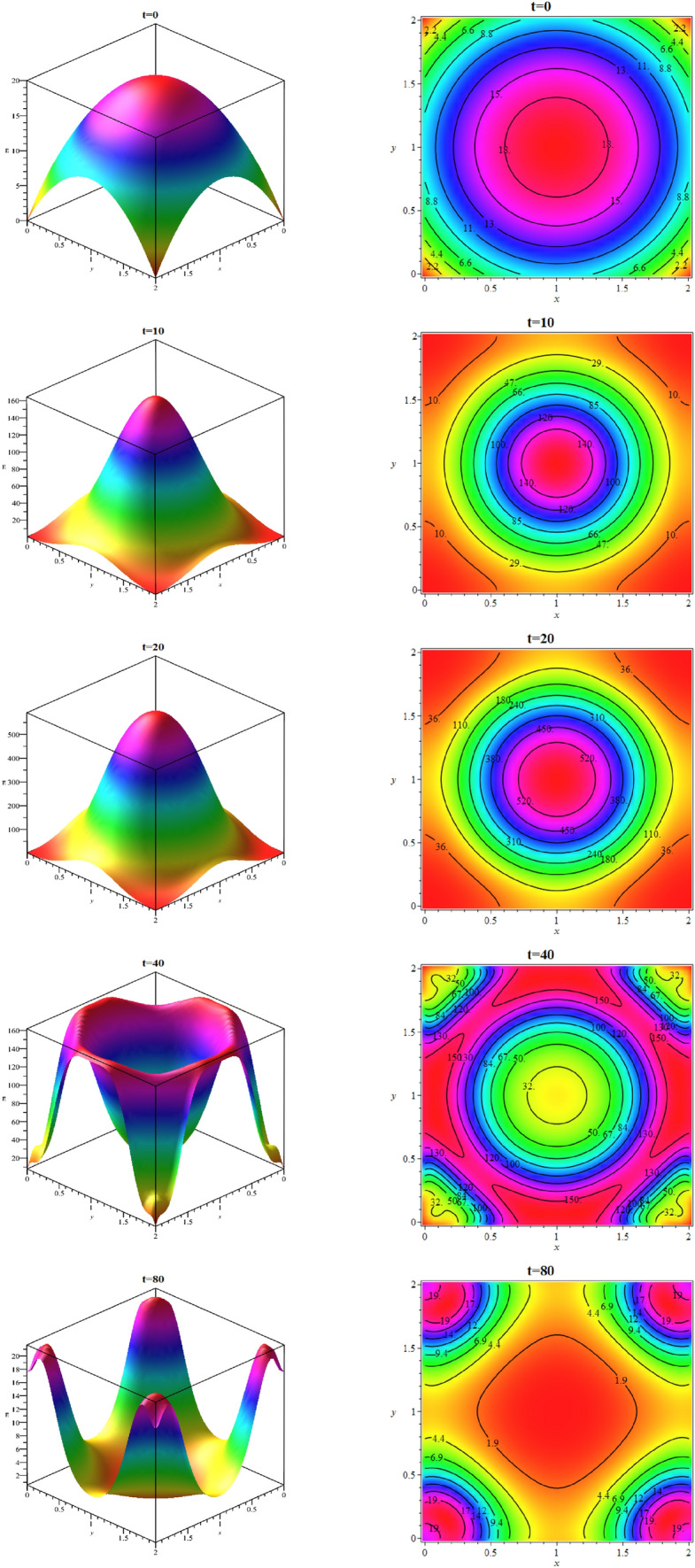
Simulating the target domain for the exposed population

Fig. 17.

Simulation of deaths in the target domain up to time $t=80$ (total)

Table 14.

Number of people exposed and deaths between 0 and 80 days for Case 7

t	0	10	20	30	40	50	60	70	80
E(t)	433	1845	7102	6803	3527	1624	795	424	236
D(t)	0	8	62	230	471	698	879	1013	1108

Conclusion

The current work has presented a computational method to solve some systems of differential equations arising from SEIHR(D)-compartment models for the Covid-19 pandemic. The technique has utilized the MLS scheme constructed on scattered points by combining the discrete Galerkin method to estimate the solution of these systems. The MLS methodology is an effective technique for the approximation of an unknown function that involves a locally weighted least squares polynomial fitting. In order to compute the integrals appeared in the method, we have used the composite Gauss–Legendre integration rule. The proposed scheme has been constructed on a set of scattered data and does not require any background cells, so it is meshless. The numerical results for different cases in confronting Covid-19 have been reported to show the validity and the efficiency of the method. Finally, as a future research, a question is raised that would it be possible to define a problem based on the raw numeric geographic data (for instance, using latitude/longitude coordinates together with case counts) and solve it using the presented method? Investigating such questions can open the way for favorable research works in this area.

Declarations

Conflict of interest

The authors declare that they have no conflict of interest.

References

- 1.Arqub OA, Maayah B. Numerical algorithm for solving time-fractional partial integrodifferential equations subject to initial and Dirichlet boundary conditions. Numer Methods Partial Differ Equ. 2018;34:1577–1597. doi: 10.1002/num.22209. [DOI] [Google Scholar]
- 2.Arqub OA, Al-Smadi M, Shawagfeh N. Solving Fredholm integro-differential equations using reproducing kernel Hilbert space method. Appl Math Comput. 2013;219(17):8938–8948. [Google Scholar]
- 3.Assari P, Dehghan M. A meshless method for the numerical solution of nonlinear weakly singular integral equations using radial basis functions. Eur Phys J Plus. 2017;132:1–23. doi: 10.1140/epjp/i2017-11467-y. [DOI] [Google Scholar]
- 4.Assari P, Dehghan M. Solving a class of nonlinear boundary integral equations based on the meshless local discrete Galerkin (MLDG) method. Appl Numer Math. 2018;123:137–158. doi: 10.1016/j.apnum.2017.09.002. [DOI] [Google Scholar]
- 5.Assari P, Dehghan M. The numerical solution of two-dimensional logarithmic integral equations on normal domains using radial basis functions with polynomial precision. Eng Comput. 2017;33(4):853–870. doi: 10.1007/s00366-017-0502-5. [DOI] [Google Scholar]
- 6.Bellomo N, Bingham R, Chaplain MA, Dosi G, Forni G, Knopoff DA, Lowengrub J, Twarock R, Virgillito ME. A multiscale model of virus pandemic: heterogeneous interactive entities in a globally connected world. Math Models Methods Appl Sci. 2020;30:1591–1651. doi: 10.1142/S0218202520500323. [DOI] [PMC free article] [PubMed] [Google Scholar]
- 7.Belytschko T, Lu YY, Gu L. Element-free Galerkin methods. Int J Numer Methods Eng. 1994;37(2):229–256. doi: 10.1002/nme.1620370205. [DOI] [Google Scholar]
- 8.Bernoulli D (1982) Reflexions sur les avantages de l’inoculation. Mercure de France, 173–190, 1760. Also in: Die Werke von Daniel Bernoulli, Band 2. Birkhauser, Basel, pp 268–274
- 9.Bertrand F, Pirch E (2021) Least-squares finite element method for a meso-scale model of the spread of COVID-19. Computation:1–22
- 10.Chen YH, Farnham PG, Hicks KA, Sansom SL. Estimating the HIV effective reproduction number in the united states and evaluating HIV elimination strategies. J Public Health Manag Pract. 2022;28(2):152–161. doi: 10.1097/PHH.0000000000001397. [DOI] [PubMed] [Google Scholar]
- 11.Chen W, Fu Z, Chen CS. Recent advances in radial basis function collocation methods. Berlin: Springer; 2014. [Google Scholar]
- 12.Cuomo S, Galletti A, Giunta G, Starace A (2013) Surface reconstruction from scattered point via GBF interpolation on GPU. In: 2013 Federated conference on computer science and information systems, pp 433–440
- 13.Cuomo S, Galletti A, Giunta G, Marcellino L. Reconstruction of implicit curves and surfaces via RBF interpolation. Appl Numer Math. 2017;116:157–171. doi: 10.1016/j.apnum.2016.10.016. [DOI] [Google Scholar]
- 14.d’Alembert J (1761) Onzieme memoire, Sur l’application du calcul des probabilites a l’inoculation de la petite verole. In: Opuscules mathematiques, Tome second, David, Paris, pp 26–95. books.google.com
- 15.Decaro N, Mari V, Elia G, Addie DD, Camero M, Lucente MS, et al. Recombinant canine coronaviruses in dogs. Europe Emerg Infect Dis. 2010;16(1):41–47. doi: 10.3201/eid1601.090726. [DOI] [PMC free article] [PubMed] [Google Scholar]
- 16.Diekmann O, Heesterbeek JAP, Metz JAJ. On the definition and the computation of the basic reproduction ratio in models for infectious diseases in heterogeneous populations. J Math Biol. 1990;28:365–382. doi: 10.1007/BF00178324. [DOI] [PubMed] [Google Scholar]
- 17.Fasshauer GE (2007) Meshfree approximation methods with MATLAB. In: Interdisciplinary mathematical sciences 6
- 18.Fasshauer GE (2005) Meshfree methods. In: Handbook of theoretical and computational nanotechnology. American Scientific Publishers, New York
- 19.Fu Z, Chen W, Ling L. Method of approximate particular solutions for constant- and variable-order fractional diffusion models. Eng Anal Bound Elem. 2015;57:37–46. doi: 10.1016/j.enganabound.2014.09.003. [DOI] [Google Scholar]
- 20.Fu Z, Chen W, Yang H. Boundary particle method for Laplace transformed time fractional diffusion equations. J Comput Phys. 2013;235:52–66. doi: 10.1016/j.jcp.2012.10.018. [DOI] [Google Scholar]
- 21.Fu Z, Xi Q, Chen W, Cheng AH-D. A boundary-type meshless solver for transient heat conduction analysis of slender functionally graded materials with exponential variations. Comput Math Appl. 2018;76(4):760–773. doi: 10.1016/j.camwa.2018.05.017. [DOI] [Google Scholar]
- 22.Feng WZ, Yang K, Cui M, Gao XW. Analytically-integrated radial integration bem for solving three-dimensional transient heat conduction problems. Int Commun Heat Mass Transf. 2016;79:21–30. doi: 10.1016/j.icheatmasstransfer.2016.10.010. [DOI] [Google Scholar]
- 23.Gao XW, Zhang Ch, Guo L. Boundary-only element solutions of 2D and 3D nonlinear and nonhomogeneous elastic problems. Eng Anal Bound Elem. 2007;31:974–982. doi: 10.1016/j.enganabound.2007.05.002. [DOI] [Google Scholar]
- 24.Grave M, Viguerie A, Barros GF, Reali A, Coutinho ALGA. Assessing the Spatio-temporal Spread of COVID-19 via Compartmental Models with Diffusion in Italy, USA, and Brazil. Arch Comput Method E. 2021;28:4205–4223. doi: 10.1007/s11831-021-09627-1. [DOI] [PMC free article] [PubMed] [Google Scholar]
- 25.Guan WJ, Ni ZY, Hu Y, Liang WH, Ou CQ, He JX, et al. Clinical characteristics of coronavirus disease 2019 in China. N Engl J Med. 2020;382(18):1708–1720. doi: 10.1056/NEJMoa2002032. [DOI] [PMC free article] [PubMed] [Google Scholar]
- 26.Guo RY, Cao DQ, Hong ZS, Tan YY, Chen SD, Jin HJ, et al. The origin, transmission and clinical therapies on coronavirus disease 2019 (COVID-19) outbreak—an update on the status. Mil Med Res. 2020;7(1):2020. doi: 10.1186/s40779-020-00240-0. [DOI] [PMC free article] [PubMed] [Google Scholar]
- 27.Guo J, Jung JH. Radial basis function ENO and weno finite difference methods based on the optimization of shape parameters. J Sci Comput. 2017;70(2):551–575. doi: 10.1007/s10915-016-0257-y. [DOI] [Google Scholar]
- 28.Guo J, Jung JH. A RBF-WENO finite volume method for hyperbolic conservation laws with the monotone polynomial interpolation method. Numer Math. 2017;122:27–50. doi: 10.1016/j.apnum.2016.10.003. [DOI] [Google Scholar]
- 29.He D, Dushoff J, Day T, Ma J, Earn DJ. Inferring the causes of the three waves of the 1918 in uenza pandemic in England and Wales. Proc R Soc B Biol Sci. 2013;280(1766):20131345. doi: 10.1098/rspb.2013.1345. [DOI] [PMC free article] [PubMed] [Google Scholar]
- 30.Hosono Y, Ilyas B. Traveling waves for a simple diffusive epidemic model. Math Models Methods Appl Sci. 1995;05(07):935–966. doi: 10.1142/S0218202595000504. [DOI] [Google Scholar]
- 31.Krishna MV, Prakash J. Mathematical modelling on phase based transmissibility of coronavirus. Infect Dis Model. 2020;5:375–385. doi: 10.1016/j.idm.2020.06.005. [DOI] [PMC free article] [PubMed] [Google Scholar]
- 32.Lancaster P, Salkauskas K. Surfaces generated by moving least squares methods. Math Comput. 1981;37(155):141–158. doi: 10.1090/S0025-5718-1981-0616367-1. [DOI] [Google Scholar]
- 33.Li MY. An introduction to mathematical modeling of infectious diseases. Mathematics of planet earth. Berlin: Springer; 2018. [Google Scholar]
- 34.Li X. Meshless Galerkin algorithms for boundary integral equations with moving least square approximations. Appl Numer Math. 2011;61(12):1237–1256. doi: 10.1016/j.apnum.2011.08.003. [DOI] [Google Scholar]
- 35.Li X, Li S. On the stability of the moving least squares approximation and the element-free Galerkin method. Comput Math Appl. 2016;72:1515–1531. doi: 10.1016/j.camwa.2016.06.047. [DOI] [Google Scholar]
- 36.Li X, Zhu J. A meshless Galerkin method for Stokes problems using boundary integral equations. Comput Methods Appl Mech Eng. 2009;198:2874–2885. doi: 10.1016/j.cma.2009.04.009. [DOI] [Google Scholar]
- 37.Li X, Zhu J. A Galerkin boundary node method and its convergence analysis. J Comput Appl Math. 2009;230(1):314–328. doi: 10.1016/j.cam.2008.12.003. [DOI] [Google Scholar]
- 38.Li X, Zhu J. A Galerkin boundary node method for biharmonic problems. Eng Anal Bound Elem. 2009;33(6):858–865. doi: 10.1016/j.enganabound.2008.11.002. [DOI] [Google Scholar]
- 39.Lohner R, Antil H, Idelsohn S, Onate E. Detailed simulation of viral propagation in the built environment. Comput Mech. 2020;66(5):1093–1107. doi: 10.1007/s00466-020-01881-7. [DOI] [PMC free article] [PubMed] [Google Scholar]
- 40.Nishiura H, Linton NM, Akhmetzhanov AR (2020) Serial interval of novel coronavirus (2019-nCoV) infections. medRxiv [DOI] [PMC free article] [PubMed]
- 41.Olivares A, Staffetti E. Uncertainty quantification of a mathematical model of COVID-19 transmission dynamics with mass vaccination strategy. Chaos Solit Fract. 2021;146:110895. doi: 10.1016/j.chaos.2021.110895. [DOI] [PMC free article] [PubMed] [Google Scholar]
- 42.Rong S, Yang L, Chu H, Fan M. Effect of delay in diagnosis on transmission of covid-19. Math Biosci Eng. 2020;17(3):2725–2740. doi: 10.3934/mbe.2020149. [DOI] [PubMed] [Google Scholar]
- 43.Siraj-Ul-Islam R, Vertnik B. Sarler, Local radial basis function collocation method along with explicit time stepping for hyperbolic partial differential equations. Appl Numer Math. 2013;67:136–151. doi: 10.1016/j.apnum.2011.08.009. [DOI] [Google Scholar]
- 44.Siraj-ul-Islam R, Sarler B, Vertnik R, Kosec G. Radial basis function collocation method for the numerical solution of the two-dimensional transient nonlinear coupled Burgers’ equations. Appl Math Model. 2012;36:1148–1160. doi: 10.1016/j.apm.2011.07.050. [DOI] [Google Scholar]
- 45.Sladek J, Sladek V, Atluri SN. Local boundary integral equation (LBIE) method for solving problems of elasticity with nonhomogeneous material properties. Comput Mech. 2000;24(6):456–462. doi: 10.1007/s004660050005. [DOI] [Google Scholar]
- 46.Smith DR. Responding to global infectious disease outbreaks: Lessons from SARS on the role of risk perception, communication and management. Soc Sci Med. 2006;63(2):3113–3123. doi: 10.1016/j.socscimed.2006.08.004. [DOI] [PMC free article] [PubMed] [Google Scholar]
- 47.Storgatz SH. Nonlinear dynamics and chaos: with application to physics, biology, chemistry and engineering. New York: Perseus Books; 1994. [Google Scholar]
- 48.Tenforde MW, Self WH, Gaglani M, et al. Effectiveness of mRNA vaccination in preventing COVID-19-associated invasive mechanical ventilation and death-United States. MMWR Morb Mortal Wkly Rep. 2022;71:459. doi: 10.15585/mmwr.mm7112e1. [DOI] [PMC free article] [PubMed] [Google Scholar]
- 49.Thompson MG, Stenehjem E, Grannis S, et al. Effectiveness of Covid-19 vaccines in ambulatory and inpatient care settings. N Engl J Med. 2021;85:1355. doi: 10.1056/NEJMoa2110362. [DOI] [PMC free article] [PubMed] [Google Scholar]
- 50.Vasileiou E, Simpson CR, Shi T, et al. Interim findings from first-dose mass COVID-19 vaccination roll-out and COVID-19 hospital admissions in Scotland: a national prospective cohort study. Lancet. 2021;397:1646. doi: 10.1016/S0140-6736(21)00677-2. [DOI] [PMC free article] [PubMed] [Google Scholar]
- 51.Viguerie A, Lorenzo G, Auricchio F, Baroli D, Hughes TJR, Patton A, Reali A, Yankeelov TE, Veneziani A. Simulating the spread of COVID-19 via a spatially-resolved susceptible-exposed-infected-recovered-deceased (SEIRD) model with heterogeneous diffusion. Appl Math Lett. 2021;111:106617. doi: 10.1016/j.aml.2020.106617. [DOI] [PMC free article] [PubMed] [Google Scholar]
- 52.Wang L, Chen JS, Hu HY. Subdomain radial basis collocation method for fracture mechanics. Int J Numer Methods Eng. 2010;83(7):851–876. doi: 10.1002/nme.2860. [DOI] [Google Scholar]
- 53.Wang L, Wang Z, Qian Z. A meshfree method for inverse wave propagation using collocation and radial basis functions. Comput Methods Appl Mech Eng. 2017;322(1):311–350. doi: 10.1016/j.cma.2017.04.023. [DOI] [Google Scholar]
- 54.Wendland H. Scattered data approximation. New York: Cambridge University Press; 2005. [Google Scholar]
- 55.Weiss SR, Navas-Martin S. Coronavirus pathogenesis and the emerging pathogen severe acute respiratory syndrome coronavirus. Microbiol Mol Biol Rev. 2005;69(4):635–664. doi: 10.1128/MMBR.69.4.635-664.2005. [DOI] [PMC free article] [PubMed] [Google Scholar]
- 56.Wu A, Peng Y, Huang B, Ding X, Wang X, Niu P, et al. Genome composition and divergence of the novel coronavirus (2019-nCoV) originating in China. Cell Host Microbe. 2020;27(3):325–328. doi: 10.1016/j.chom.2020.02.001. [DOI] [PMC free article] [PubMed] [Google Scholar]
- 57.Xu S, Huang R, Sy LS, et al. COVID-19 vaccination and non-COVID-19 mortality risk-seven integrated health care organizations. MMWR Morb Mortal Wkly Rep. 2021;70:1520. doi: 10.15585/mmwr.mm7043e2. [DOI] [PMC free article] [PubMed] [Google Scholar]
- 58.Yang D, Leibowitz JL. The structure and functions of coronavirus genomic 3’ and 5’ ends. Virus Res. 2015;206:120–133. doi: 10.1016/j.virusres.2015.02.025. [DOI] [PMC free article] [PubMed] [Google Scholar]
- 59.Yang C, Wang J. A mathematical model for the novel coronavirus epidemic in Wuhan, China. Math Biosci Eng. 2020;17(3):2708–2724. doi: 10.3934/mbe.2020148. [DOI] [PMC free article] [PubMed] [Google Scholar]
- 60.You C, Deng Y, Hu W, Sun J, Lin Q, Zhou F et al (2020) Estimation of the time-varying reproduction number of 180 COVID-19 outbreak in China. medRxiv. https://www.medrxiv.org/content/early/181 2020/02/17/2020.02.08.20021253 [DOI] [PMC free article] [PubMed]
- 61.Zhao L, Wang ZC. Traveling wave fronts in a diffusive epidemic model with multiple parallel infectious stages. IMA J Appl Math. 2016;81:795–823. doi: 10.1093/imamat/hxw033. [DOI] [Google Scholar]
- 62.Zhou P, Yang XL, Wang XG, et al. A pneumonia outbreak associated with a new coronavirus of probable bat origin. Nature. 2020;579:270. doi: 10.1038/s41586-020-2012-7. [DOI] [PMC free article] [PubMed] [Google Scholar]
- 63.Zohdi T. Modeling and simulation of the infection zone from a cough. Comput Mech. 2020;66(4):1025–1034. doi: 10.1007/s00466-020-01875-5. [DOI] [PMC free article] [PubMed] [Google Scholar]
- 64.Zohdi T (2020) Rapid simulation of viral decontamination efficacy with irradiation. Comput Methods Appl Mech Eng 369 [DOI] [PMC free article] [PubMed]