Abstract
It is well known in the literature that human behavior can change as a reaction to disease observed in others, and that such behavioral changes can be an important factor in the spread of an epidemic. It has been noted that human behavioral traits in disease avoidance are under selection in the presence of infectious diseases. Here, we explore a complementary trend: the pathogen itself might experience a force of selection to become less “visible,” or less “symptomatic,” in the presence of such human behavioral trends. Using a stochastic SIR agent-based model, we investigated the co-evolution of two viral strains with cross-immunity, where the resident strain is symptomatic while the mutant strain is asymptomatic. We assumed that individuals exercised self-regulated social distancing (SD) behavior if one of their neighbors was infected with a symptomatic strain. We observed that the proportion of asymptomatic carriers increased over time with a stronger effect corresponding to higher levels of self-regulated SD. Adding mandated SD made the effect more significant, while the existence of a time-delay between the onset of infection and the change of behavior reduced the advantage of the asymptomatic strain. These results were consistent under random geometric networks, scale-free networks, and a synthetic network that represented the social behavior of the residents of New Orleans.
Keywords: Mandated social distancing, Self-regulated social distancing, Network, Viral evolution, Symptomatic variant, Asymptomatic variant
Introduction
Epidemic spread of infectious diseases is a topic that has received much attention among computational modelers, see, e.g., Ma and Xia (2009), Diekmann et al. (2012), Siettos and Russo (2013), Heesterbeek et al. (2015), Cobey (2020). One important aspect of this process is the rise and spread of mutant variants of the pathogen (Feng et al. 2006; Day et al. 2011; Poletto et al. 2013, 2015; Griette et al. 2015; Gandon et al. 2016). For example, in a spatially expanding epidemic, it was shown that less virulent strains will dominate the periphery while more virulent strains will prevail at the core (Osnas et al. 2015). It has also been observed that in epidemic models where infection events happen on an interaction network, evolutionary dynamics of the pathogen change depending on the structure of the network (Newman 2005; Karrer and Newman 2011; Bansal and Meyers 2012; Miller 2013). It has been shown, for example, that heterogeneities in contact structure (i.e., network degree) may accelerate the spread of a single disease, and at the same time slow down the rise of a rare advantageous mutation under susceptible–infected–susceptible (SIS) infection dynamics (Leventhal et al. 2015). In the context of spatial networks with host migration, it was reported that the spatial network structure may have important effects on the transient evolutionary dynamics during an epidemic (Lion and Gandon 2016); in particular, the front and the rear of the expanding epidemic are expected to be phenotypically different. Pinotti et al. (2019) studied the influence of the social network structure on competition dynamics of strains (with identical parameters) that are spread via a stochastic SIS model on the network. It was found that network structure can affect the ecology of pathogens: in a more heterogeneous network (a network with a high standard deviation for its degree distribution), a reduction in the number of strains and an increase in the dominance of one strain were observed, while strong community structure (a set of nodes in a network, which are strongly connected to each other, have few or no connection with nodes out of the set) in the social network increased the strain diversity.
Another relevant characteristic of epidemic dynamics that has been investigated is the effect of human behavior on disease spread, see, e.g., Funk et al. (2010), Eksin et al. (2017), Eksin et al. (2019), Weitz et al. (2020). Different aspects of human behavior have been considered, including relational exchange (e.g., replacement of sick individuals by healthy ones in the workplace) (Scarpino et al. 2016), people’s hygiene (Fewtrell et al. 2005), voluntary vaccination and vaccination compliance (Bauch and Earn 2004), “risky” versus “careful” individual behavior (Del Valle et al. 2005; Tanaka et al. 2002; Epstein et al. 2008; Gross et al. 2006; Funk et al. 2009), and the related concept of social distancing. Social distancing is a change of behavior that can roughly be classified into (1) self-regulated (or spontaneous) where individuals may choose to limit their contacts based on information that they receive or on their personal beliefs (Ariful Kabir et al. 2019; Kan and Zhang 2017; Funk et al. 2009; Sun et al. 2011; Wang et al. 2015; Wu et al. 2012); and (2) mandated (public), where the decrease in social contacts is regulated centrally and affects either the entire population or certain subpopulations (Glass et al. 2006; Valdez et al. 2012). The COVID-19 pandemic has triggered much research into the role of social distancing in viral spread, especially because before the advance of vaccination, non-pharmaceutical intervention (NPI) measures were the only intervention available (Lewnard and Lo 2020). NPI policies have taken a variety of forms such as extreme lockdowns, school closures, road and transit systems restrictions, and mandatory isolation/quarantine (Kupferschmidt and Cohen 2020), see, e.g., Feng et al. (2020), Vokó and Pitter (2020), Chowdhury et al. (2020), Kissler et al. (2020), Ferguson et al. (2020), Koo et al. (2020), Hellewell et al. (2020), Gatto et al. (2020), Wang et al. (2020), Liu et al. (2020), Li et al. (2020) on the effects of mandated social distancing on SARS-CoV-2 spread. In a recent paper Huang et al. (2021), the authors considered the combination of both mandated and self-regulated types of social distancing, and studied their effect on the outbreak threshold of an (asymptomatic) infectious disease.
In this paper, we explore the role of mandated and self-regulated social distancing on viral evolution. The focus of this study is the co-evolution of two types of a pathogen: the resident, more symptomatic, pathogen, and an emerging, less symptomatic (or asymptomatic), variant. The two may or may not differ in their infectivity properties, but because they present differently, they will trigger different behavior by individuals, which may result in different levels of self-regulated social distancing. As a result, the less symptomatic variant may experience a selective advantage. We will use the usual framework of the susceptible–infectious–removed (SIR) model on networks, and investigate how the network structure (including random networks of different types and a synthetic network representing social interactions of real individuals) modifies the co-dynamics of the two viral strains.
Methods
The agent-based model (ABM) describes the infection transmission dynamics and intervention strategies. It is assumed that the disease spreads within a susceptible–infected–removed (SIR) framework. Dynamics take place on a network, and three different network types are studied.
Network Structure
We assume that the epidemic spreads on a network of size N, where each node represents a person, and the edges represent interactions. Here, we study two types of random, unweighted networks: the random geometric network, and the scale-free network (each with nodes). Each of these networks represents a different type of abstraction that retains certain features of human interactions. In addition to these two theoretical random networks, we studied disease spread on a real-world synthetic network of a much larger size (), where the edges are weighted by the time the two individuals spend together. This synthetic network was constructed based on interaction data of people in New Orleans (Eubank et al. 2010, 2008).
Random Spatial-Geometric Network This network is constructed by placing N points in a unit square and connecting only the points that are within a prescribed Euclidean distance, r, from each other. Such networks are characterized by strong local structure and clustering properties, and have been studied extensively (Dall and Christensen 2002; Lang et al. 2018). Such networks could represent local social contacts of individuals in the absence of any long-range connections.
Scale-Free Network This network is characterized by a power law degree distribution. As a result, while most individuals only have a limited number of contacts, there are “super-spreaders” with very high degrees (Barabási and Bonabeau 2003; Barabási and Albert 1999). Examples of applications of such networks are the number of sexual partners in a college environment (Crawford 1990) or the network of a city with buildings (nodes) and flows of people as connecting edges (Chowell et al. 2003).
We use Networkx open software platform (Hagberg et al. 2004) to generate spatial-geometric random networks in dimension 2 with a distance threshold . We also use the Barabási–Albert preferential attachment model in Networkx to generate scale-free networks with degree distribution . The random networks have the same size and average degree, but they differ in terms of their degree distributions and other properties, since they have different structures.
Each of these networks has advantages and disadvantages when used to model epidemic spread in populations. Random spatial-geometric networks successfully model the clustering properties of human interactions but do not include long-range connections or super-spreaders. Super-spreaders are a natural part of scale-free networks, but the latter network type has no clustering or neighborhood structure. For these reasons, we perform all the analyses for different network types, to investigate whether observed phenomena depend on any particular network properties. Finally, we implement the most realistic network in the study, the New Orleans synthetic network, which is described below.
Real-World Network Our real-world network is based on the synthetic data generated by Simfrastructure (Eubank et al. 2010, 2008) for synthetic people residing in New Orleans. This network is generated by sampling the real-world data of New Orleans individual activity and contacts. The network statistically reflects the demographics of New Orleans and the social connections of the city’s population. Simfrastructure is a high-performance, service-oriented, agent-based modeling and simulation system for representing and analyzing interdependent infrastructures. In the New Orleans network, each edge ij between two nodes i and j is weighted by , which represents the strength of connectivity between i and j, and reflects the type of connection as well as the amount of time the two individuals spend with each other.
SIR Model on a Network for Two Virus Strains
In our stochastic SIR agent-based model (ABM), an individual i at time t is either susceptible to being infected, infected, or removed from the infection because of recovery or death. During a time-interval , an infected individual can infect any of its susceptible neighbors (that is, susceptible individuals connected with the infected individual by an edge). We denote by the infection rate per edge, such that during time , the probability that a susceptible individual j will be infected by an infected neighbor i is given by . (Note that for the random spatial and scale-free networks, we will use ). For each infected individual, a recovery event occurs during the time-interval with probability , or a death event occurs with probability , and we refer to the rate of death or recovery as the rate of removal, .
We assume the existence of two distinct variants (strains) of the virus, which we denote by and . Our model incorporates permanent cross-immunity for either viruses, that is, if an individual is infected by virus k, then the individual is immune to virus for during infection and after recovery (here ). We further assume that an individual infected with virus k can only induce infection with virus k, that is, we do not consider spontaneous mutations from one type of virus to the other.
Unless noted otherwise, the two virus strains are assumed to have identical parameters, that is, the same values of and . The only difference between the two strains is that one () causes a symptomatic disease, while the other () is asymptomatic. This variation in expression gives rise to differences in people’s behavior, as described in the next subsection. Later on, we consider scenarios in which symptomatic infection is coupled to a higher viral infectivity.
For initialization, we start the epidemic by randomly infecting one individual with . We then advance the simulation until the epidemic grows to 0.1% -infected individuals. At this time, we introduce the next randomly generated newly infected case as a infection; this represents a single mutation event of the resident strain.
At this point, we reset the time to zero and use this state as the initial condition to study the virus co-dynamics in the absence of any further mutant generation.
Simulation speed depends on the time-step size , so it is desirable to pick the largest value for such that the simulations exhibit reasonable convergence accuracy, see also Roche et al. (2011). We have implemented the program for the null scenario (no social distancing) with values representing 1 day, 1 h, and 1 min, and while results differed significantly between day and h, the result for h and min was almost identical. Therefore, we chose h for our simulations in this study.
Social Distancing Strategies
We model two types of social distancing (SD) strategies: (1) mandated SD implemented by the government, and (2) self-regulated SD.
Mandated SD is implemented as follows: When the prevalence of virus (i.e., the fraction of infected individuals among the population) reaches a fixed threshold , all individuals start practicing temporary social distancing. To this end, a fraction of all the edges in the network is removed for consecutive days; connections to be removed are chosen randomly.
Self-regulated SD is also implemented only if the number of infections has reached the threshold prevalence . If an individual has at least one neighbor that is symptomatically infected with (after a delay following infection), the individual removes a fraction of his/her connections. The connections to be removed are chosen randomly, and remain cut for as long as there is a symptomatically infected neighbor.
It is possible that the fraction or of connections is a non-integer number, K. In this case, if [K] stands for the integer part of K, connections are removed with probability , and [K] connections are removed otherwise.
Parameter Values
The definitions of all the variables and parameters of the proposed model are given in Table 1. The parameter values have been chosen to be realistic for respiratory infections and are specified in the figure legends. Under these parameters, the basic reproduction number is between 2 and 3 for the examples considered.
Table 1.
Parameter and state variable definitions and notations
| Notation | Description | Unit | |
|---|---|---|---|
| N | Number of nodes in the network | People | |
| Network | Spatial network | – | |
| Parameters | Scale-free random network | – | |
| Real-world network | – | ||
| The connectivity level between two neighbors i and j | 1 | ||
| Average number of contact per time for random networks | Contact/time | ||
| Prob. of transmission per contact per time for individuals contacting viral strain | 1/contact | ||
| Infection | Per time removal (death or recovery) probability from virus k | 1/time | |
| Parameters | Time period between infection and development of symptoms for individuals infected with viral strain | Time | |
| Prevalence threshold: Infection prevalence to start SD | 1 | ||
| Intervention | Mandated SD: fraction of removed contacts | 1 | |
| Parameters | Self-regulated SD against : fraction of removed contacts | 1 | |
| Duration of mandated SD | Time |
Here, SD stands for social distancing
To estimate the basic reproduction number , starting with a randomly selected individual as the initial infected case, we count the number of neighbors who are subsequently infected by the focal individual during the infectious period. We repeat this process for a large number of independent simulations, seeding each one with a different initially infected individual.
Intervention parameters will change based on different scenarios explored here, and are specified in figure legends.
Results: Positive Selection of the Asymptomatic Strain on Different Networks
Here, we explore the consequences of behavioral changes (self-regulated social distancing) on the spread of an asymptomatic viral strain. This is first done by using two types of abstract random networks, the scale-free and the random spatial network. Both types of random networks have some features resembling different aspects of human social networks. Then, we show how similar scenarios play out on a more realistic network that emulates the behavior of a real-life population of New Orleans.
Self-Regulated Social Distancing Selects for an Asymptomatic Strain
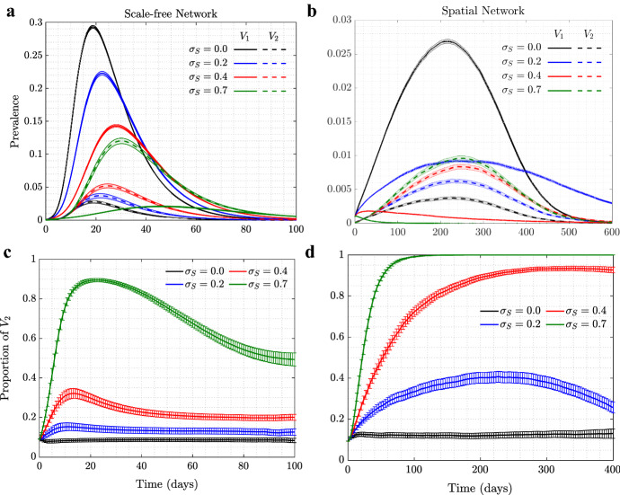
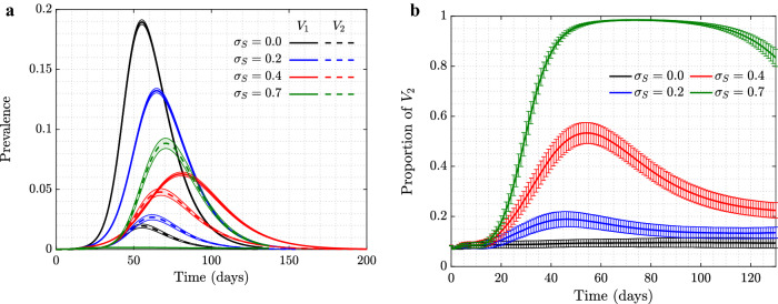
In our model, individuals in the population exercise self-regulated SD if members of their circle become symptomatically infected (that is, become infected with ). To explore the consequence of this behavior on the evolutionary dynamics of asymptomatic virus variants (), we ran simulations where such a mutant was introduced as a minority in the initial stages of the epidemic, see Fig. 1. We explored the dynamics on two different networks: scale-free (left panels) and spatial (right panels); the trajectories and the error bars are averages and standard deviations over 5000 independent simulations. We present four different degrees of self-regulated SD: (a control case where is indistinguishable from in the model, and no selection is expected), (low-degree self-regulated SD), (moderate self-regulated SD), and (high-degree self-regulated SD). As time goes by and the epidemic spreads, we plot the prevalence of each virus (panels (1a) and (1b)), and also follow the relative share of , that is (panels (1c) and (1d)).
Fig. 1.
(Color figure online) The role of self-regulated SD in the spread of viruses. Time series are shown for four scenarios: No (, black), low (, blue), moderate (, red), and high (, green) self-regulated SD, and in the absence of mandated SD. Scale-free (left) and spatial (right) networks of 10, 000 individuals with average degree 10 are used. a, b The prevalence of (solid) and (dashed); c, d the proportion of (). The remaining parameters are per day, , per day per contact for the scale-free and per day per contact for the spatial network (corresponding to ). Means and standard errors are shown for 5000 stochastic realizations
In the absence of self-regulated SD (black lines in panels (1a) and (1b)), the epidemic on the two networks looks different despite similar parameters: infection burns through the scale-free network faster and reaches a higher infection peak, while in the case of the spatial network it lasts longer at relatively low levels.
Under zero self-regulated SD (black lines in panels (1c) and (1d)), as expected, the proportion of remains approximately constant throughout the course of the epidemic, although we do observe an initial increase in the abundance of in the spatial network. This initial increase is due to a somewhat “advantageous” initial location of the infection. In the spatial network, the individuals initially infected with are placed on the “outskirts” of the growing infected neighborhood, which results in a larger mean number of uninfected neighbors that -infected individuals have compared to -infected individuals. This initial increase of the proportion of is therefore due to the initial placement and does not represent an ongoing selection.
A different pattern is observed in the presence of self-regulated SD: the proportion of infected individuals increases well beyond the initial boost. This effect is stronger for a larger extent of self-regulated SD (compare green () to red () to blue () lines in the bottom panels of Fig. 1). The exact extent to which the fraction of increases in the course of the epidemic depends, besides , on the network size and type. Larger networks will result in a larger increase in fraction, simply because they experience a larger and longer epidemic, and will have a longer time to gain on before the epidemic runs out of targets (not shown); a similar result can be demonstrated by using an ODE model of an SIR infection with two viral strains, see “Appendix 1.”
We note a significant difference in the amount of gain experienced by the asymptomatic strain under scale-free (panel (c)) and spatial (panel (d)) networks. Self-regulated SD results in much more effective protection on a spatial network, because if an individual has an infected neighbor, the first individual is likely to have more than one infected neighbor, and self-regulated SD induced by one of the neighbors will work against future infections in the vicinity. This spatial inhibition results in a much larger force of selection experienced by the asymptomatic strain on a spatial network, compared to the case of scale-free network, which does not have a community structure. More details are presented in “Appendix 2.”
Advantage Mediated by Self-Regulated SD Can Offset a Fitness Cost of the Asymptomatic Strain
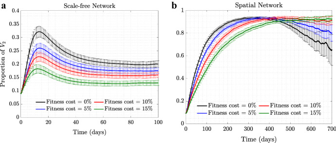
Figure 2 explores a scenario where the asymptomatic mutant, , has a fitness cost compared to the resident virus, , which is manifested through a reduction in the probability of transmission parameter. We can see that although having a small disadvantage in reduces the fraction of , we still observe a rise in the prevalence of caused by self-regulated SD against symptomatic cases. In other words, the behavior-based selection mechanism can work even in the presence of a degree of disadvantage in the transmissibility of the mutant compared to the resident type. We observe that even in the presence of a significant fitness disadvantage for virus , self-regulated SD can provide enough pressure to lead to positive selection of the asymptomatic virus.
Fig. 2.
(Color figure online) Selection for in the presence of a fitness cost. Time series of proportion of under moderate self-regulated SD, (and with ), are shown for fitness cost (, black), fitness cost (, blue), fitness cost (, red), and fitness cost (, green), for a scale-free and b spatial networks. All the other parameters are as in Fig. 1
Again, we note a difference in the force of selection for the asymptomatic strain under scale-free and spatial networks. In the case of a scale-free network, (Fig. 2a) a 15% disadvantage of almost completely eliminates any advantage gained through self-regulated SD. In the case of a spatial network (Fig. 2b), an asymptomatic strain with a 15% fitness costs still rises to almost 90% in the population.
Mandated Social Distancing Makes Selection Stronger
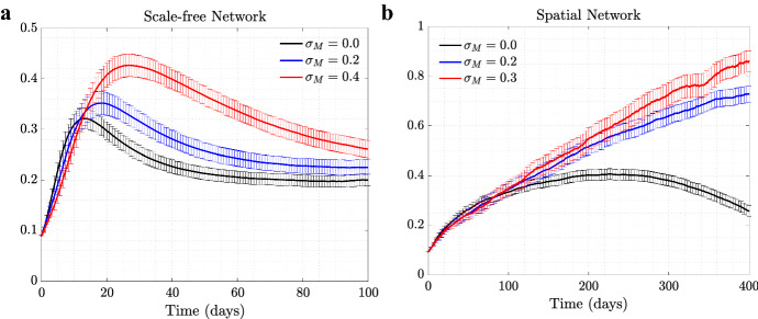
Next, we explored the consequence of mandated SD implementation on the selection for the asymptomatic strain. Mandated SD affects transmission of both viral strains equally, and it is not immediately clear whether the presence of mandated SD can modify the dynamics and change the advantage experienced by through self-regulated SD. Figure 3 assumes the presence of self-regulated SD at an intermediate level, and shows that increasing the level of mandated SD increases the positive selection pressure experienced by the asymptomatic strain.
Fig. 3.
(Color figure online) The effect of mandated SD on the proportion of . The proportion of the asymptomatic strain, , is shown as a function time, for three different levels of mandated SD: a Scale-free network, (black), (blue), and , with ; b spatial network, (black), (blue), and (red), with . All the other parameters are as in Fig. 1. The levels for mandated and self-regulated SD are selected in such a way that remains above one so an outbreak for is observed
To explain some of the patterns observed in our ABM network model, we will turn to SIR models based on ordinary differential equations (ODEs). Such models are an important tool in epidemiological infection studies (Anderson and May 1992), and they have been widely used for various emerging infections such as COVID-19 (Fang et al. 2020). Here, we denote by x the fraction of susceptible individuals, and distinguish between two strains of infection, and . The fraction of individuals infected with is denoted by and the fraction of individuals infected with is denoted by . We assume that an individual cannot be superinfected with a different virus, and that recovered individuals have permanent immunity. These assumptions give rise to the following system:
| 1a |
| 1b |
| 1c |
where and and with initial conditions
Here and are the rate of infection for the two strains, and the rate of removal. Let us denote by z the proportion of the individuals infected with :
This quantity satisfies the following equation:
| 2 |
In particular, if the two strains are neutral to each other () then the fraction z is expected to stay constant. It will increase if and decrease if . In the presence of self-regulated and mandated SD of strengths and , respectively, we can express the infectivity of the two viral strains as
with which Eq. (2) becomes
| 3 |
To investigate how the dynamics of z change with the degree of mandated SD, we note that the only -dependent part of the right-hand side of Eq. (3) is the product . Initially, , and this quantity decays with , that is, we expect that the proportion of the mutant infection grows more slowly under higher degrees of mandated SD. This behavior is indeed what we observe initially in Fig. 3 (other instances of this behavior appear in Figs. 7b and 12b in the appendix). As the epidemic progresses, the number of susceptible individuals (x) decreases, but the amount of decrease depends on the level of mandated SD: the value of x will be higher for higher and lower for lower . As a result, the dynamics of z is under the influence of two competing factors: (1) the infectivity is lower for higher values of , and (2) the population of susceptibles is higher for higher values of . Both numerical simulations (“Appendix 1”) and analytical calculations in the limit of a large time separation of the two infections (“Appendix 1”) show that the overall tendency for the quantity is to increase with .
Fig. 7.
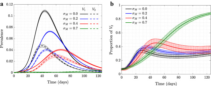
(Color figure online) New Orleans Network of size 150, 000 individuals: the role of mandated SD in the spread of viruses. Time series are shown for four scenarios of no (, black), low (, blue), moderate (, red), and high (, green) mandated SD, in the presence of moderate self-regulated SD (). a plot is the prevalence of (solid) and (dashed); b shows the proportion of (). and all the other parameters are as in Fig. 1 (corresponding to ). Means and standard errors are shown for 1000 stochastic realizations
Fig. 12.
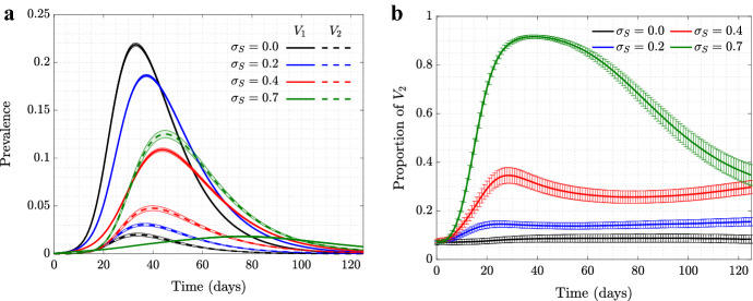
(Color figure online) New Orleans Network under school closure: the role of self-regulated SD in the spread of viruses. Time series are shown for four scenarios of no (, black), low (, blue), moderate (, red), and high (, green) self-regulated SD, in the absence of mandated SD. a Plot is the prevalence of (solid) and (dashed); b shows the proportion of (). and all the other parameters are as in Fig. 1 in the main text (corresponding to ). Means and standard errors are shown for 1000 stochastic realizations
Further patterns of wild-type and mutant virus co-dynamics are investigated in the Appendix. In particular, “Appendix 2” discusses differences in the behavior exhibited by network models compared to ODEs, and “Appendix 4” explores parameter dependence of the mutant fraction, as well as the final epidemic size of the two viral strains.
The Effect of Time-Lag on -Selection
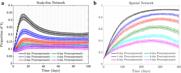
All the simulations shown so far assumed that self-regulated SD behavior was triggered in an individual as soon as a -infected individual became infectious; i.e., there is no pre-symptomatic infection period and the infection status is known instantly. In reality, however, there could be a delay between a neighbor’s infection and a change in response behavior, caused by a delayed onset of symptoms, delayed testing, or a lag in information spread. Figure 4 explores the scenario where a number of days passes between an infection event and the time when self-regulated SD starts.
Fig. 4.
(Color figure online) The effect of delay of self-regulated SD on selection of . The proportion of is shown as time series for the a scale-free and b spatial network, in the presence of time delay in the appearance of symptoms when infected by . The different colors correspond to time delays of 0, 1, , 5 days. Here, , , and the rest of the parameters are as in Fig. 1
We can see that a delay reduces positive selection experienced by the asymptomatic strain. Under scale-free networks, for the parameters in Fig. 4, in the presence of a 5-day lag, the non-delay scenario increase in the fraction of is almost completely eliminated. Again, because the positive selection for is much stronger under spatial networks, we still observe a significant rise in the fraction of in panel (b) even in the presence of a 5-day delay in symptom onset.
Co-dynamics of Strains on the New Orleans Social Network
Thus far we have investigated the co-dynamics of viral strains on two random networks, scale-free and spatial. Both reflect different features of human interaction networks, but possess many very different mathematical properties. All of the major results were consistent across both networks. As the next step, we will use a real-world network to demonstrate that the same trends continue to hold there.
The synthetic network that we employ here was constructed to statistically match the demographics of New Orleans residents, based on the 2009 census data. Of approximately 400, 000 residents living in 190, 000 households, the synthetic network’s sample contains 150, 000 individuals. These individuals comprise the set of network nodes, and the edges represent contacts of synthetic individuals through various activity types, such as “home,” “work,” “school,” and “shopping.” The network statistically reflects the social connections of the city’s population. Each edge of the network is labeled with one of the activity types and contains information on the amount of time spent on these contacts per day, resulting in a weighted network (Eubank et al. 2010, 2008). We assumed that the amount of contact time necessary to cause an infection event is 15 min (or 0.01 of day, which is based on COVID-19 data Keeling et al. (2020)); therefore, we removed all edges with weight less than 0.01. The resulting network has average degree 15.82 and average clustering coefficient 0.32. The degree distribution of this synthetic network is shown in Fig. 5. To further parameterize the model, we chose the same removal probability as in the random networks studied above, and adjusted the probability of transmission to obtain .
Fig. 5.
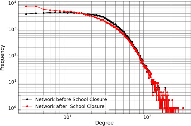
(Color figure online) Degree distribution of the New Orleans synthetic network. Red: the basic network; black: the network under school closure (see “Appendix 3”). The network includes 150, 000 nodes and has average degree 15.82 (with average degree 12.67 under school closure)
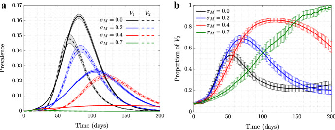
Figure 6 presents the time series of prevalence of the two viruses and the proportion of under different levels of self-regulated SDs, in the absence of mandated SD. As established with the two types of random networks, the presence of self-regulated SD confers selective advantage to the asymptomatic virus strain, . We observe that self-regulated SD at level reduces the peak of the symptomatic strain, , to less than half, and at level it reduces the peak of by about a factor of 10, while the impact on the peak of is much more modest. The proportion of in the right panel of Fig. 6 increases to a peak, and this effect is stronger for higher levels of self-regulated SD. These results are consistent with those obtained for the random networks.
Fig. 6.
(Color figure online) New Orleans Network of size 150, 000 individuals: the role of self-regulated SD in the spread of viruses. Time series are shown for four scenarios of no (, black), low (, blue), moderate (, red), and high (, green) self-regulated SD, in the absence of mandated SD. a plot is the prevalence of (solid) and (dashed); b shows the proportion of (). and all the other parameters are as in Fig. 1 (corresponding to ). Means and standard errors are shown for 1000 stochastic realizations
Figure 7 explores the effect of mandated SD in the presence of an intermediate-level self-regulated SD, . Again, the results are consistent with those observed for random networks. Increasing the level of mandated SD can make the selection for significantly stronger.
Discussion
It has been reported in the literature that human behavior can change as a reaction to disease observed in others, see, e.g., Andersson-Ellström et al. (1996), Darrow (1997), Hays (2005), Curtis (2014), Azizi et al. (2020), Komarova et al. (2021). It has further been emphasized that such behavioral changes can be an important factor in epidemic spread, e.g., in the context of sexually transmitted diseases (Hadeler and Castillo-Chávez 1995; Hyman and Li 1997), or more generally (Funk et al. 2010; Eksin et al. 2017, 2019; Weitz et al. 2020). It has been noted that human behavioral traits in disease avoidance are under selection in the presence of infectious diseases (Tanaka et al. 2002). Here, we explore a complementary trend: the pathogen itself might experience a force of selection to become less “visible,” or less “symptomatic,” in the presence of such human behavioral trends.
We used a discrete-time stochastic network model to investigate the spread of two co-circulating virus strains, one of which () is symptomatic and the other () asymptomatic. The resident strain () is assumed to give rise to a mutant strain () sometime during the epidemic. Three types of networks are studied: scale-free and spatial random networks, and a real-world synthetic network statistically describing social activity of individuals in New Orleans. We implemented two types of social distancing, self-regulated SD and mandated SD. Under mandated social distancing, individuals cut a given fraction of their contacts randomly, while in self-regulated social distancing, individuals opt to protect themselves based on the infection status of their contacts. More precisely, individuals cut some of their connections randomly if they find a symptomatically infected individual among their contacts.
We observed that in the presence of self-regulated protection against symptomatic cases (self-regulated SD), the proportion of asymptomatic carriers increased over time with a stronger effect corresponding to higher levels of self-regulated SD. Adding mandated SD made the effect even more significant: the proportion of increased for a longer duration of time and reached a higher maximum in the presence of mandated SD. Interestingly, the intensity of these trends was higher for the spatial (more homogeneous and clustered) network compared with the scale-free network, which was a result of more local infection spread and community structure. When the simulations were repeated for the real-world social network based on the New Orleans data, the selection effect was more similar to that observed for the scale-free than for the spatial network.
The selection effects observed could be weakened, e.g., by the existence of an inherent fitness disadvantage of (as a result, for example, of a lower infectivity of this strain), or by a time delay that exists between the onset of infection and the change of behavior triggered under self-regulated SD. Nonetheless, we have shown that even in the presence of these factors the selective advantage of the asymptomatic strain resulting from human behavior can still be significant and lead to a noticeable shift in the prevalence of this virus type.
While our model suggests that cautious human behavior can select for a virus variant that is less symptomatic, this selection pressure can in principle also lead to more complex outcomes. A similar advantage would be gained if the onset of symptoms was delayed and if the host could transmit the virus during this prolonged pre-symptomatic phase. Such a virus variant would also evade the behavioral reduction of network connections, yet this variant does not have to be less symptomatic or be less pathogenic. This property might be at work to some extent with the SARS-CoV-2 delta variant, which is characterized by a longer window between testing positive and developing symptoms compared to previous variants (Kang et al. 2021). Although the delta variant appears to produce higher viral loads than previous variants (Li et al. 2021), which alone can lead to a significant transmission advantage, the longer duration of an infectious pre-symptomatic phase of delta can lead to a strong amplification of this advantage if people adjust their behavior solely in response to symptomatic social contacts. This mechanism might be an important contributor to the rapid rise of the delta variant across the globe.
The model presented here is a simplification of reality. Modeling human behavior is challenging, and here we ignored many complexities by, for example, assuming that individuals remove connections probabilistically when learning of a symptomatically infected individual among their circle of contacts. This approach does not distinguish between prolonged contacts with friends and brief contacts such as encounters in a supermarket. It also ignores demographic and socioeconomic factors that may alter the extent to which individuals can adopt new behaviors to avoid getting infected. In addition, a static network of contacts has been assumed while in reality individuals may not have the same contacts every time unit.
Despite these uncertainties, our analysis shows robustly that human behavior in response to an infection outbreak can modulate the evolutionary trajectory of the virus. In particular, a cautious reaction of people to personal contacts that display symptomatic disease can promote the emergence of virus strains that induce less symptomatic disease, and we have argued that the delta variant of SARS-CoV-2 arose from this mechanism. While we have not modeled one particular infection, the modeling approach is geared to describing generic respiratory infections that are transmitted through casual social contact, and therefore has implications for the current SARS-CoV-2 pandemic.
Appendix A: The Effect of Mandated Social Distancing: An ODE Model
We can use ODE modeling of the type (1–1c) to explore the effect of mandated SD on the dynamics of the asymptomatic strain.
Let us consider the problem where is an advantageous mutant (), which is initially in a minority, that is, . From the equation for the mutant fraction, see (2), we note that in this case, z will be an increasing function of time. Its initial growth is exponential with the rate approximately given by (assuming that ). As x decreases, the growth slows down. Two extreme scenarios can be distinguished, see Fig. 8:
z approaches 1 well before x decreases significantly; in this case the dynamics of z is well described by the logistic growth model.
The epidemic ends well before z approaches 1, in which case near the epidemic end, the growth of z becomes linear with the rate approximately given by , where is the final epidemic size.
We observe that larger overall values of corresponds to a more modest expansion of the advantageous virus (assuming that the % advantage is fixed; it is for example in Fig. 8).
Fig. 8.
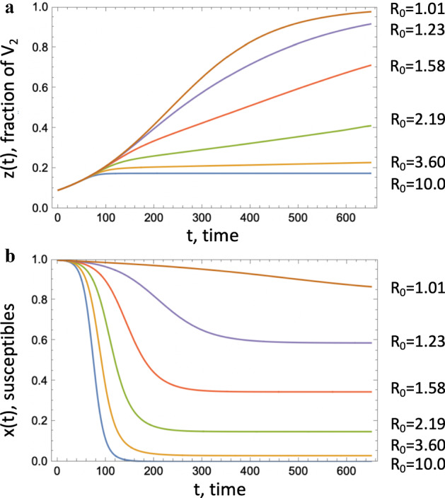
Fraction of an advantageous virus, . a The quantity z(t) obtained by solving Eqs. (1–1c) is plotted as a function of time for several values of , obtained by changing the death rate, a. b The corresponding susceptible populations as functions of time. The rest of the parameters are
In this context, it is useful to calculate the value
If , then we have the following final size relation:
which is an implicit formula for . In the case of two different pathogens, if we denote , we have Arino et al. (2007)
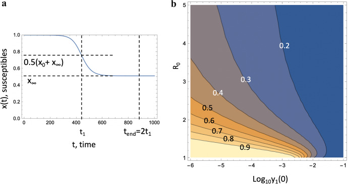
The ODE model can be used to calculate the proportion of by the end of epidemic. Figure 9 shows an example where we fixed the values and , such that has a advantage in terms of infectivity, and also assumed that . Parameters and were varied over a wide range, which corresponds to varying (associated with the resident virus) and the total population size relative to the initial number of infected individuals. Panel (a) illustrates the way we numerically calculate the end of epidemic time, , and panel (b) shows the fraction of at time as a function of and .
Fig. 9.
(Color figure online) Fraction of at the end of the epidemic. a Calculation of , which represents the end of the epidemic, is illustrated. The blue line is the fraction of susceptible individuals, x(t), obtained as a solution of Eqs. (1–1c); , where corresponds to . In other words, at time the population of susceptible individuals reaches halfway to its final value, . b Quantity obtained by solving Eqs. (1–1c), is plotted at time , as a function of the initial proportion of individuals infected with , and . The rest of the parameters are
We observe that typically, increasing leads to a smaller final fraction of . For relatively large values, the fraction of susceptible individuals decreases quickly leading to an extremely slow linear growth of the fraction z(t). On the other hand, decreasing (which is equivalent to considering larger total populations) leads to an increase in the final fraction of . Larger populations result in a longer epidemic, and consequently has a longer time to gain on .
Appendix B: The Case of Time Separation Between Wild-Type and Mutant Infections
In the ODE model, the dynamics of the mutant fraction, z, is described by Eqs. (2) or (3). The dependence on in the right-hand side of this equation is through the term
| 4 |
In “Appendix 1,” we showed numerically that as increases (which is equivalent of decreasing), F increased, resulting in an enhanced growth of advantageous mutants. In this section, we will prove this result in a special case of a time-separated epidemic.
Figure 10a shows an example of a system that experiences two epidemic peaks, an early one in terms of (the wild type epidemic) and then a later one in terms of (the mutant epidemic). This happens in this particular ODE model because the initial conditions for and satisfy , that is, at time , the abundance of the mutant is significantly lower than that of the wild type. In this case, first the wild type infection experiences a peak of , which is then followed by a second, delayed peak of a mutant infection. In a sense, the fact that the mutant strain is introduced at a relatively low level compared to the wild type strain causes a delay of the epidemic caused by the mutant virus.
Fig. 10.
Illustration of time-separated epidemics. a Numerical solution of system (1–1c) with initial conditions , where the mutant infection is characterized by an initial condition much lower than that of the wild type. The three populations are plotted as a function of time. The dashed lines show the system behavior in the absence of the mutant, and in particular, the quantity is shown. b Numerical solutions of system (–) with for and system (8–10) with for . The other parameters are
To gain understanding of the dynamics, we can study a simplified system that exhibits a similar behavior. Figure 10b shows a scenario where the mutant strain is introduced after the wild type strain has already burned through the population. Suppose the wild type strain satisfies the usual system,
and the initial conditions are given by . The final epidemic size,
is given by Harko et al. (2014), Komarova et al. (2021)
| 5 |
where u is the solution of
| 6 |
The fraction of susceptible individuals left by the first epidemic is then given by
| 7 |
Note that is a decreasing function of (the higher the infectivity, the fewer susceptibles are left). The second epidemic can then be described by the system
| 8 |
| 9 |
| 10 |
with the initial conditions imposed at some time T after the first wave of the epidemic has passed: . The growth rate for the infected individuals in Eq. (9) is given by
Note that this growth rate is positive only if the advantage of the virus (factor ) is sufficiently high. would like to investigate the dependence of the quantity on the mandated distancing, which enters the expressions through . To assess the sign of the dependence, it is enough to consider the function F defined in (4), and in the current setting can be approximated as
We can see that while decreases with , it is not immediately clear whether the product increases or decreases. From Eqs. (5) and (7),
and we have
| 11 |
Differentiating Eq. (6) respect to and resolving for , we obtain
Using this in (11), we obtain
| 12 |
where
First let us show that
| 13 |
To get an upper bound on u, we will use a well-known inequality, which, when substituted into (6), gives
For this is equivalent to
On the other hand, we have
where the last inequality follows from the fact that is the initial fraction of susceptible individuals. Therefore, we conclude that inequality (13) holds.
To determine the sign of the derivative in (12), we notice that (this is the condition for the first epidemic to take off), and . Therefore, , and together with inequality (13), we obtain from (12) that
In other words, the growth rate of the mutant virus, , decreases with . This means that as mandated SD, , increases, this leads to a decrease in , which in turn causes to increase. Thus, ma
ndated SD increases the growth rate of a delayed, advantageous infection.
Appendix C: Further Details of Viral Co-Dynamics
In Fig. 1, as well as others (such as Figs. 3, 2), we observe that the fraction of often has a one-humped shape: it first increases to a peak and then decreases as the epidemic dwindles down. This is a phenomenon that does not have an analogy in the simple ODE model, (1–1c). Equation (2) for the fraction suggests that the proportion of always increases if . On the other hand, in the agent-based models for symptomatic virus and its asymptomatic counterpart, , we observe that, both for scale-free and spatial networks, the numerical gain of eventually decreases. This is related to the epidemic duration of the two strands: the advantageous virus experiences a shorter epidemic, and this effect increases with the amount of advantage. Figure 11 shows that the time it take to reach its infection peak is shorter compared to that for , and as we increase the level of self-regulated SD (thus increasing the advantage of ), the difference in the peak time grows. Therefore, there is a time-interval during which the amount of infection already decreases while still grows toward its peak, resulting in a reduction in the fraction.
Fig. 11.
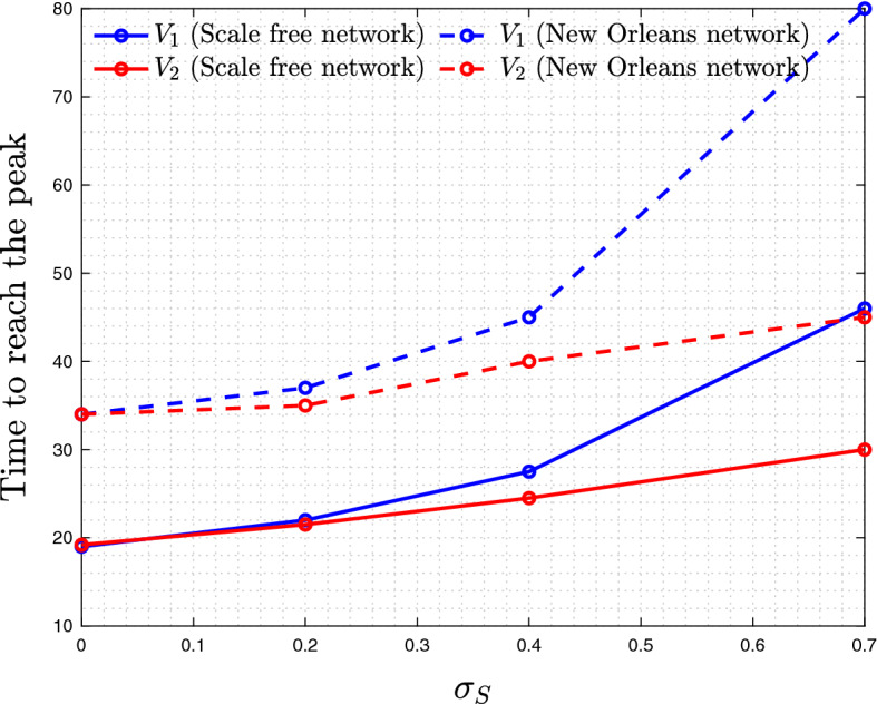
(Color figure online) Time to reach infection peak for viruses (blue) and (red), as a function of (the measure of advantage)
Note that this is not observed in the ODE system and also was less pronounced in more clustered spatial network. In ODE model, the peak of infection is reached when , which corresponds to the time when , for . Since x(t) is a decreasing function and (in analogy with self-regulated SD), we necessarily conclude that , that is, the epidemic corresponding to a more infectious type is always longer.
Appendix D: Co-Dynamics of Strains on New Orleans Social network Under School Closure
School closure is an important component of social distancing measures, which has for example been implemented widely during the SARS-CoV-2 pandemic. Therefore, we have repeated the analysis of Sect. 3.5 after removing all the edges related to “school.” Degree distribution of the resulting network is shown in black in Fig. 5. We tuned up the transmission rates and to have and reran our simulations on the new network, see Figs. 12 and 13.
Fig. 13.
(Color figure online) New Orleans Network under school closure: the role of mandated SD in the spread of viruses. Time series are shown for four scenarios of no (, black), low (, blue), moderate (, red), and high (, green) mandated SD, in the presence of moderate self-regulated SD (). a plot is the prevalence of (solid) and (dashed); b shows the proportion of (). and all the other parameters are as in Fig. 1 in the main text (corresponding to ). Means and standard errors are shown for 1000 stochastic realizations
In Fig. 12, we implemented the impact of various levels for self-regulated SD ( and 0.7) in the absence of mandated SD (). Similar to previous results, increasing the level of self-regulated SD causes more selective advantage to the asymptomatic virus strain, .
Figure 13 explores the effect of mandated SD in the presence of an intermediate-level self-regulated SD, . Again, and similar to the results of Sect. 3.5, increasing the level of mandated SD causes that the selection for to become significantly stronger.
While the results for the New Orleans Network are qualitatively similar with and without school closure, we notice that the effect of further SD measures on the background of closed schools is stronger, since we start with a somewhat sparser network.
Appendix E: Parameter Dependence of the Results
Here, we present simulation results that show how the viral co-dynamics change with system parameters.
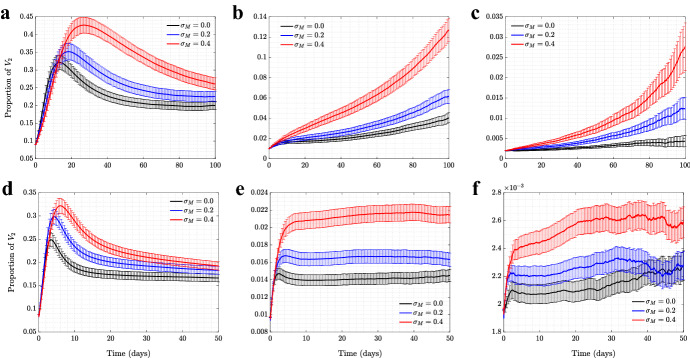
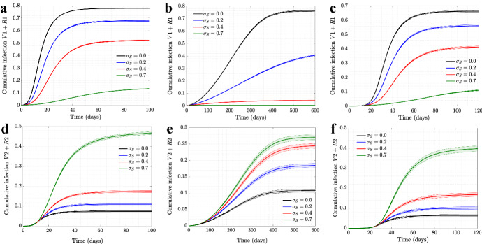
Figure 14 plots the proportion of mutant infections as a function of time, and shows results for six different scenarios. The top row panels correspond to a lower overall transmission rate ( per day) and the bottom panels to a higher transmission rate ( per day). Further, we investigate the role of initial conditions: from left to right the ratio takes values 0.1, 0.01, and 0.002. Shown is the impact of different levels of mandated SD (, and 0.4) for the fixed level of self-regulated SD (), for the dynamics on a scale-free network.
Fig. 14.
The effect of mandated SD on the proportion of for scenarios of low/high transmission rate and different initial conditions. The proportion of the asymptomatic strain, , is shown as a function time, for 3 different levels of mandated SD () and fixed positive level of self-regulated SD () on scale-free network: a per day and ; b per day and ; c per day and ; d per day and ; e per day and ; and f per day and . All the other parameters are as in Fig. 1. The levels for mandated and self-regulated SD are selected in such a way that remains above one so an outbreak for is observed
We observe that in all cases, increasing the level of mandated SD () enhances the asymptomatic mutant. Decreasing causes larger separation between the peaks of and (Turkyilmazoglu 2021), and therefore, the proportion of stays higher for a longer time. On the other hand, increasing transmission rate reduces the advantage of as a result of both types of SDs.
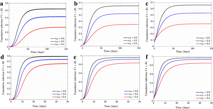
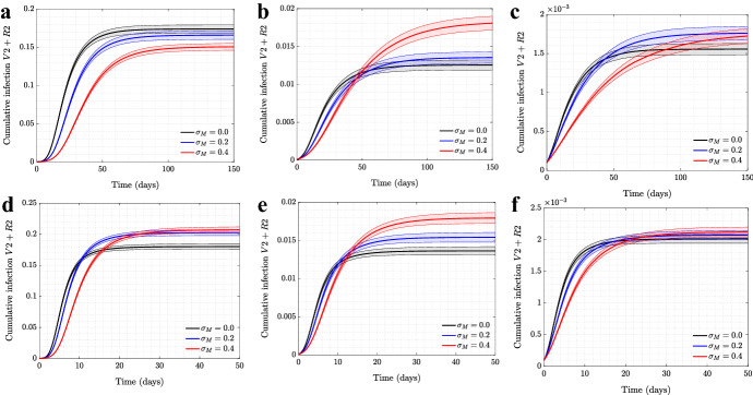
Figures 15 and 16 show the cumulative infection for the wild type and mutant virus, respectively. We observe, not surprisingly, that the total number of infections decreases with the level of mandated SD, see Fig. 15. On the other hand, the influence of on the dynamics of is less straightforward. In Fig. 16, we can see that for relatively small infectivity and a larger initial proportion of the mutant virus (panel (a)), higher values of result in a lower number of individuals infected with the mutant virus. Decreasing the initial proportion of reverses this effect (panels (b,c)). To explain this we note that as the quantity decreases (left to right), the peaks of and become more and more separated, approaching the scenario described in “Appendix 1.” As was shown analytically, in the limit of a large time separation of the two epidemics, the growth rate of the advantageous mutant will increase with mandated SD, which is consistent with the patterns in Figs. 16)b, c. In the absence of this separation, the two epidemics are nearly concurrent, and mandated SD affects both viruses in the same way, reducing the total number of infections (panel (a)).
Fig. 15.
The effect of mandated SD on cumulative infection of symptomatic strain for scenarios of low/high transmission rate and different initial conditions. The cumulative infection for symptomatic strain, , is shown as a function time, for six different levels of mandated SD () and fixed positive level of self-regulated SD () on scale-free network. The parameters for a–f are as in Fig. 14
Fig. 16.
The effect of mandated SD on cumulative infection of asymptomatic strain for scenarios of low/high transmission rate and different initial conditions. The cumulative infection for asymptomatic strain, , is shown as a function time, for six different levels of mandated SD () and fixed positive level of self-regulated SD () on scale-free network. The parameters for a–f are as in Fig. 14
Note that for a higher overall infectivity (Fig. 16d–f), for all three choices of the initial conditions, the two epidemics are sufficiently separated in time to exhibit behavior patterns studied in “Appendix 1.” This is because higher values of result in faster, shorter epidemic waves, such that even the initial ratio leads to the first wave subsiding significantly before the second one takes off.
For completeness, we also investigated the role of self-regulated SD on the cumulative numbers of infections for the wild type virus (the top row of Fig. 17) and for the mutant virus (the bottom row). Three types of networks are shown (from left to right): scale-free, spatial, and the synthetic New Orleans network. In all cases, as the level of self-regulated SD increases, the total number of asymptomatic cases increases, with a corresponding decrease in the number of symptomatic cases. This is the result of an increased advantage of as we increase the value of .
Fig. 17.
The effect of self-regulated SD on cumulative infection of symptomatic/asymptomatic strains for various network structures. The cumulative infections for are shown as a function time, for four different levels of self-regulated SD () and no mandated SD (), simulated on a, d scale-free network; b, e spatial network; c, f New Orleans network. All the other parameters are as in Fig. 1 for a–e and Fig. 6 for c, f
In Figs. 15–17, we also can capture the behavior of final epidemic size for each virus depending on different levels of SD strategies. For instance, while increasing mandated SD decreases final size of (see Fig. 15), the final size of does not have a monotonic response to SD, that is, mandated SD can increase or decreases the final size of depending on the transmission parameters and SD intensity (see Fig. 16).
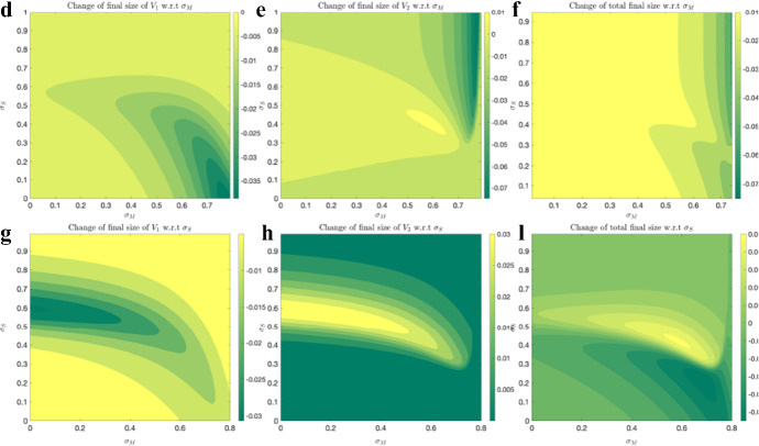
To investigate these behaviors with more details, we ran the ODE version of our model, (1–1c), for different levels of social distancing, and . Figure 18 shows final size of , final size of and total final size (summation of final size of , and final size of ) as functions of and values, over their range [0, 1]. Here, we assume , , , , and the maximum value of is chosen so that .
Fig. 18.
Final sizes versus SD levels: the model in (1–1c) is used to quantify the amount of final sizes for (a), (b), and both (c), for different levels of SD strategies ( and ). The parameter values are , , and for initial condition we have and , thus
In the panel A of Fig. (18), we observe that final size of decreases in both x and y directions, indicating that this characteristic always decreases with increase in social distancing, that is, both mandated and self-regulated SD are successful in controlling final size of . In panel (B), we observe that final size of always increases in y direction, that is, increasing self-regulated SD causes an increase in final size of . However, in x direction, final size of can be both increasing or decreasing, indicating that the final epidemic size of may end up larger for higher level of mandated SD, depending on the social distancing parameter values. Total final size (in panel (C)) decreases in x direction, indicating that it always decreases with mandated SD; however, it may be increasing in y direction, similarly indicating that the total epidemic size may end up larger for higher levels of self-regulated SD, depending on the social distancing parameter values. These observations become more clear if we plot the partial derivatives of final sizes with respect to and , as shown in Fig. 19.
Fig. 19.
Change in final sizes with respect to SD levels: The same model and parameter values as the one in Fig. (18) are used to quantify the change of final sizes with respect change of SD strategies
The color bars in Fig. 19 indicate both positive and negative values for only two panels of six plots, (E) and (I), which correspond to the two interesting cases stated above:
Higher mandated social distancing may lead to a higher epidemic size for .
Higher self-regulated social distancing may lead to a higher total epidemic size.
These outcomes are only observed for a subset of values on the plane.
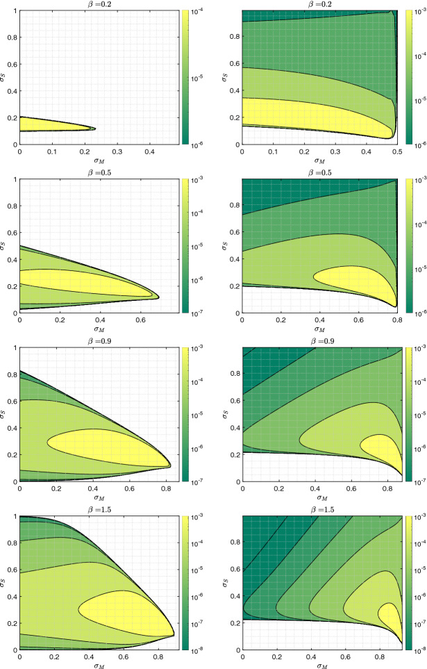
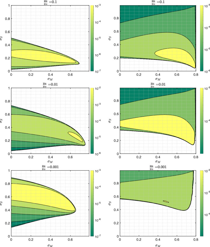
Furthermore, these results depend on transmission rate and initial infection ratios . Figure 20 shows the regions where observations (1) and (2) hold, for various transmission rates, , and Fig. 21 shows these regions for initial conditions, . First columns indicate the regions for which higher mandated SD () leads to a higher final epidemic size for . The second columns indicate the regions for which higher self-regulated SD leads to higher total final epidemic size, and lighter colors indicate higher rates of increase.
Fig. 20.
The region for which final epidemic sizes increase as a result of social distancing, for various transmission rates: The same model and recovery rate as those in Fig. (18), initial condition , (), and various transmission rates are used. The left column shows the region of SD parameter values, for which final epidemic size of increases with increasing mandated SD. The right column shows the region of SD parameter values, for which total final epidemic size increases with increasing self-regulated SD
Fig. 21.
The region for which final epidemic sizes increase as a result of social distancing for various initial conditions: The same model and infection parameters as those in Fig. (18), but various initial conditions are used. The left column shows the region of SD parameter values, for which final epidemic size of increases with increase in mandated SD. The right column shows the region of SD parameter values, for which total final epidemic size increases with increase in self-regulated SD
In Fig. 20 (the first column), the size of the colored region increases with the transmission rate ; indicating that if the transmission rate is high, mandated SD is likely to lead to a higher final epidemic size for . In its second column, the size of the colored region is large for all transmission rate values, and occupies , indicating that some self-regulated SD helps decrease the total epidemic size. However, beyond a critical value ( here), any increase in self-regulated SD is likely to increase total final epidemic size. Looking closer, we observe that the region is not only larger for lower values, but also the rate of increase is higher, indicating that this negative effect of self-regulated SD on the total epidemic size is stronger for lower transmission rates.
In the first column of Fig. 21, we observe that the size of the colored region is non-monotonic as the initial condition decreases. This result is consistent with result in Fig. 16, indicating that for relatively smaller values of , mandated SD is likely to lead to a higher final epidemic size for , unless the value for initial is much lower than that of , which causes separation of epidemics discussed in “Appendix 1.” In its second column, on the other hand, we see that the critical value for increases as decreases.
Funding
This research was supported through the MIDAS Coordination Center (MIDASUGP2020-2) by a grant from the National Institute of General Medical Science (3U24GM132013-02S2), and NSF DMS 1662146/1662096.
Footnotes
Publisher's Note
Springer Nature remains neutral with regard to jurisdictional claims in published maps and institutional affiliations.
References
- Anderson RM, May RM. Infectious diseases of humans: dynamics and control. Oxford: Oxford University Press; 1992. [Google Scholar]
- Andersson-Ellström A, Forssman L, Milsom I. The relationship between knowledge about sexually transmitted diseases and actual sexual behaviour in a group of teenage girls. Sex Transm Infect. 1996;72(1):32–36. doi: 10.1136/sti.72.1.32. [DOI] [PMC free article] [PubMed] [Google Scholar]
- Ariful Kabir KM, Kuga K, Tanimoto J. Effect of information spreading to suppress the disease contagion on the epidemic vaccination game. Chaos Solitons Fractals. 2019;119:180–187. [Google Scholar]
- Arino J, Brauer F, van den Driessche P, Watmough J, Jianhong W. A final size relation for epidemic models. Math Biosci Eng. 2007;4(2):159. doi: 10.3934/mbe.2007.4.159. [DOI] [PubMed] [Google Scholar]
- Azizi A, Montalvo C, Espinoza B, Kang Y, Castillo-Chavez C. Epidemics on networks: reducing disease transmission using health emergency declarations and peer communication. Infect Dis Model. 2020;5:12–22. doi: 10.1016/j.idm.2019.11.002. [DOI] [PMC free article] [PubMed] [Google Scholar]
- Bansal S, Meyers LA. The impact of past epidemics on future disease dynamics. J Theor Biol. 2012;309:176–184. doi: 10.1016/j.jtbi.2012.06.012. [DOI] [PubMed] [Google Scholar]
- Barabási A-L, Albert R. Emergence of scaling in random networks. Science. 1999;286(5439):509–512. doi: 10.1126/science.286.5439.509. [DOI] [PubMed] [Google Scholar]
- Barabási A-L, Bonabeau E. Scale-free networks. Sci Am. 2003;288(5):60–69. doi: 10.1038/scientificamerican0503-60. [DOI] [PubMed] [Google Scholar]
- Bauch CT, Earn DJD. Vaccination and the theory of games. Proc Natl Acad Sci. 2004;101(36):13391–13394. doi: 10.1073/pnas.0403823101. [DOI] [PMC free article] [PubMed] [Google Scholar]
- Chowdhury R, Luhar S, Khan N, Choudhury SR, Matin I, Franco OH. Long-term strategies to control covid-19 in low and middle-income countries: an options overview of community-based, non-pharmacological interventions. Eur J Epidemiol. 2020;35(8):743–748. doi: 10.1007/s10654-020-00660-1. [DOI] [PMC free article] [PubMed] [Google Scholar]
- Chowell G, Hyman JM, Eubank S, Castillo-Chavez C. Scaling laws for the movement of people between locations in a large city. Phys Rev E. 2003;68(6):066102. doi: 10.1103/PhysRevE.68.066102. [DOI] [PubMed] [Google Scholar]
- Cobey S. Modeling infectious disease dynamics. Science. 2020;368(6492):713–714. doi: 10.1126/science.abb5659. [DOI] [PubMed] [Google Scholar]
- Crawford I. Attitudes of undergraduate college students toward AIDS. Psychol Rep. 1990;66(1):11–16. doi: 10.2466/pr0.1990.66.1.11. [DOI] [PubMed] [Google Scholar]
- Curtis VA. Infection-avoidance behaviour in humans and other animals. Trends Immunol. 2014;35(10):457–464. doi: 10.1016/j.it.2014.08.006. [DOI] [PubMed] [Google Scholar]
- Dall J, Christensen M. Random geometric graphs. Phys Rev E. 2002;66(1):016121. doi: 10.1103/PhysRevE.66.016121. [DOI] [PubMed] [Google Scholar]
- Darrow WW. Health education and promotion for std prevention: lessons for the next millennium. Sex Transm Infect. 1997;73(2):88–94. doi: 10.1136/sti.73.2.88. [DOI] [PMC free article] [PubMed] [Google Scholar]
- Day T, Alizon S, Mideo N. Bridging scales in the evolution of infectious disease life histories: theory. Evol Int J Organ Evol. 2011;65(12):3448–3461. doi: 10.1111/j.1558-5646.2011.01394.x. [DOI] [PubMed] [Google Scholar]
- Del Valle S, Hethcote H, Hyman JM, Castillo-Chavez C. Effects of behavioral changes in a smallpox attack model. Math Biosci. 2005;195(2):228–251. doi: 10.1016/j.mbs.2005.03.006. [DOI] [PubMed] [Google Scholar]
- Diekmann O, Heesterbeek H, Britton T. Mathematical tools for understanding infectious disease dynamics. Princeton: Princeton University Press; 2012. [Google Scholar]
- Eksin C, Shamma JS, Weitz JS. Disease dynamics in a stochastic network game: a little empathy goes a long way in averting outbreaks. Sci Rep. 2017;7(1):1–13. doi: 10.1038/srep44122. [DOI] [PMC free article] [PubMed] [Google Scholar]
- Eksin C, Paarporn K, Weitz JS. Systematic biases in disease forecasting-the role of behavior change. Epidemics. 2019;27:96–105. doi: 10.1016/j.epidem.2019.02.004. [DOI] [PubMed] [Google Scholar]
- Epstein JM, Parker J, Cummings D, Hammond RA. Coupled contagion dynamics of fear and disease: mathematical and computational explorations. PLoS ONE. 2008;3(12):e3955. doi: 10.1371/journal.pone.0003955. [DOI] [PMC free article] [PubMed] [Google Scholar]
- Eubank S (2008) Synthetic data products for societal infrastructures and protopopulations: data set 2.0. Technical report, Technical Report NDSSL-TR-07-003, Network Dynamics and Simulation Science Laboratory, Virginia Polytechnic Institute and State University, 2008
- Eubank S, Barrett C, Beckman R, Bisset K, Durbeck L, Kuhlman C, Lewis B, Marathe A, Marathe M, Stretz P. Detail in network models of epidemiology: are we there yet? J Biol Dyn. 2010;4(5):446–455. doi: 10.1080/17513751003778687. [DOI] [PMC free article] [PubMed] [Google Scholar]
- Fang Y, Nie Y, Penny M. Transmission dynamics of the COVID-19 outbreak and effectiveness of government interventions: a data-driven analysis. J Med Virol. 2020;92(6):645–659. doi: 10.1002/jmv.25750. [DOI] [PMC free article] [PubMed] [Google Scholar]
- Feng Z, Glasser JW, Hill AN. On the benefits of flattening the curve: a perspective. Math Biosci. 2020;326:108389. doi: 10.1016/j.mbs.2020.108389. [DOI] [PMC free article] [PubMed] [Google Scholar]
- Feng Z, Dieckmann U, Levin SA (eds) (2006) Disease evolution: models, concepts, and data analyses, vol 71. American Mathematical Society, Providence, Rhode Island, USA
- Ferguson N, Laydon D, Nedjati Gilani G, Imai N, Ainslie K, Baguelin M, Bhatia S, Boonyasiri A, Cucunuba Perez ZU, Cuomo-Dannenburg G et al (2020) Report 9: impact of non-pharmaceutical interventions (NPIs) to reduce COVID19 mortality and healthcare demand. Imp Coll Lond 10(77482):491–497
- Fewtrell L, Kaufmann RB, Kay D, Enanoria W, Haller L, Colford Jr JM. Water, sanitation, and hygiene interventions to reduce diarrhoea in less developed countries: a systematic review and meta-analysis. Lancet Infect Dis. 2005;5(1):42–52. doi: 10.1016/S1473-3099(04)01253-8. [DOI] [PubMed] [Google Scholar]
- Funk S, Gilad E, Watkins C, Jansen VAA. The spread of awareness and its impact on epidemic outbreaks. Proc Natl Acad Sci. 2009;106(16):6872–6877. doi: 10.1073/pnas.0810762106. [DOI] [PMC free article] [PubMed] [Google Scholar]
- Funk S, Salathé M, Jansen VAA. Modelling the influence of human behaviour on the spread of infectious diseases: a review. J R Soc Interface. 2010;7(50):1247–1256. doi: 10.1098/rsif.2010.0142. [DOI] [PMC free article] [PubMed] [Google Scholar]
- Gandon S, Troy Day C, Metcalf JE, Grenfell BT. Forecasting epidemiological and evolutionary dynamics of infectious diseases. Trends Ecol Evol. 2016;31(10):776–788. doi: 10.1016/j.tree.2016.07.010. [DOI] [PubMed] [Google Scholar]
- Gatto M, Bertuzzo E, Mari L, Miccoli S, Carraro L, Casagrandi R, Rinaldo A. Spread and dynamics of the covid-19 epidemic in Italy: effects of emergency containment measures. Proc Natl Acad Sci. 2020;117(19):10484–10491. doi: 10.1073/pnas.2004978117. [DOI] [PMC free article] [PubMed] [Google Scholar]
- Glass RJ, Glass LM, Beyeler WE, Jason Min H. Targeted social distancing designs for pandemic influenza. Emerg Infect Dis. 2006;12(11):1671. doi: 10.3201/eid1211.060255. [DOI] [PMC free article] [PubMed] [Google Scholar]
- Griette Q, Raoul G, Gandon S. Virulence evolution at the front line of spreading epidemics. Evolution. 2015;69(11):2810–2819. doi: 10.1111/evo.12781. [DOI] [PubMed] [Google Scholar]
- Gross T, D’Lima CJD, Blasius B (2006) Epidemic dynamics on an adaptive network. Phys Rev Lett 96(20) [DOI] [PubMed]
- Hadeler KP, Castillo-Chávez C. A core group model for disease transmission. Math Biosci. 1995;128(1–2):41–55. doi: 10.1016/0025-5564(94)00066-9. [DOI] [PubMed] [Google Scholar]
- Hagberg A, Schult D, Swart P, Conway D, Séguin-Charbonneau L, Ellison C, Edwards B, Torrents J (2004) Networkx. High productivity software for complex networks. Webová strá nka. https://networkx.lanl.gov/wiki, 2004
- Harko T, Lobo FSN, Mak MK. Exact analytical solutions of the susceptible-infected-recovered (sir) epidemic model and of the sir model with equal death and birth rates. Appl Math Comput. 2014;236:184–194. [Google Scholar]
- Hays JN (2005) Epidemics and pandemics: their impacts on human history. Abc-clio, 2005
- Heesterbeek H, Anderson RM, Andreasen V, Bansal S, De Angelis D, Dye C, Eames KT, Edmunds WJ, Frost SD, Funk S et al (2015) Modeling infectious disease dynamics in the complex landscape of global health. Science 347(6227):aaa4339 [DOI] [PMC free article] [PubMed]
- Hellewell J, Abbott S, Gimma A, Bosse NI, Jarvis CI, Russell TW, Munday JD, Kucharski AJ, Edmunds WJ, Sun F et al (2020) Feasibility of controlling covid-19 outbreaks by isolation of cases and contacts. Lancet Glob Health 8(4):e488–e496 [DOI] [PMC free article] [PubMed]
- Huang H, Chen Y, Yan Z. Impacts of social distancing on the spread of infectious diseases with asymptomatic infection: a mathematical model. Appl Math Comput. 2021;398:125983. doi: 10.1016/j.amc.2021.125983. [DOI] [PMC free article] [PubMed] [Google Scholar]
- Hyman JM, Li J. Behavior changes in sis std models with selective mixing. SIAM J Appl Math. 1997;57(4):1082–1094. [Google Scholar]
- Kan J-Q, Zhang H-F. Effects of awareness diffusion and self-initiated awareness behavior on epidemic spreading-an approach based on multiplex networks. Commun Nonlinear Sci Numer Simul. 2017;44:193–203. doi: 10.1016/j.cnsns.2016.08.007. [DOI] [PMC free article] [PubMed] [Google Scholar]
- Kang M, Xin H, Yuan J, Ali ST, Liang Z, Zhang J, Hu T, Lau EH, Zhang Y, Zhang M et al (2021) Transmission dynamics and epidemiological characteristics of delta variant infections in China. medRxiv, 2021 [DOI] [PMC free article] [PubMed]
- Karrer B, Newman MEJ. Competing epidemics on complex networks. Phys Rev E. 2011;84(3):036106. doi: 10.1103/PhysRevE.84.036106. [DOI] [PubMed] [Google Scholar]
- Keeling MJ, Deirdre Hollingsworth T, Read JM. Efficacy of contact tracing for the containment of the 2019 novel coronavirus (covid-19) J Epidemiol Commun Health. 2020;74(10):861–866. doi: 10.1136/jech-2020-214051. [DOI] [PMC free article] [PubMed] [Google Scholar]
- Kissler S, Tedijanto C, Lipsitch M, Grad YH (2020) Social distancing strategies for curbing the covid-19 epidemic. medRxiv, 2020
- Komarova NL, Azizi A, Wodarz D. Network models and the interpretation of prolonged infection plateaus in the covid19 pandemic. Epidemics. 2021;35:100463. doi: 10.1016/j.epidem.2021.100463. [DOI] [PMC free article] [PubMed] [Google Scholar]
- Koo JR, Cook AR, Park M, Sun Y, Sun H, Lim JT, Tam C, Dickens BL (2020) Interventions to mitigate early spread of sars-cov-2 in Singapore: a modelling study. Lancet Infect Dis 20(6):678–688 [DOI] [PMC free article] [PubMed]
- Kupferschmidt K, Cohen J. Can China’s COVID-19 strategy work elsewhere? Science. 2020;367(6482):1061–1062. doi: 10.1126/science.367.6482.1061. [DOI] [PubMed] [Google Scholar]
- Lang JC, De Sterck H, Kaiser JL, Miller JC. Analytic models for SIR disease spread on random spatial networks. J Complex Netw. 2018;6(6):948–970. [Google Scholar]
- Leventhal GE, Hill AL, Nowak MA, Bonhoeffer S. Evolution and emergence of infectious diseases in theoretical and real-world networks. Nat Commun. 2015;6(1):1–11. doi: 10.1038/ncomms7101. [DOI] [PMC free article] [PubMed] [Google Scholar]
- Lewnard JA, Lo NC. Scientific and ethical basis for social-distancing interventions against covid-19. Lancet Infect Dis. 2020;20(6):631. doi: 10.1016/S1473-3099(20)30190-0. [DOI] [PMC free article] [PubMed] [Google Scholar]
- Li T, Liu Y, Li M, Qian X, Dai SY. Mask or no mask for covid-19: a public health and market study. PLoS ONE. 2020;15(8):e0237691. doi: 10.1371/journal.pone.0237691. [DOI] [PMC free article] [PubMed] [Google Scholar]
- Li B, Deng A, Li K, Hu Y, Li Z, Shi Y, Xiong Q, Liu Z, Guo Q, Zou L, Zhang H et al (2021) Viral infection and transmission in a large well-traced outbreak caused by the delta sars-cov-2 variant. MedRxiv, 2021 [DOI] [PMC free article] [PubMed]
- Lion S, Gandon S. Spatial evolutionary epidemiology of spreading epidemics. Proc R Soc B Biol Sci. 2016;283(1841):20161170. doi: 10.1098/rspb.2016.1170. [DOI] [PMC free article] [PubMed] [Google Scholar]
- Liu C, Wu X, Niu R, Wu X, Fan R (2020) A new SAIR model on complex networks for analysing the 2019 novel coronavirus (COVID-19). Nonlinear Dyn 101(3):1777–1787 [DOI] [PMC free article] [PubMed]
- Ma S, Xia Y (2009) Mathematical understanding of infectious disease dynamics, vol 16. World Scientific, Singapore
- Miller JC. Cocirculation of infectious diseases on networks. Phys Rev E. 2013;87(6):060801. doi: 10.1103/PhysRevE.87.060801. [DOI] [PMC free article] [PubMed] [Google Scholar]
- Newman MEJ. Threshold effects for two pathogens spreading on a network. Phys Rev Lett. 2005;95(10):108701. doi: 10.1103/PhysRevLett.95.108701. [DOI] [PubMed] [Google Scholar]
- Osnas EE, Hurtado PJ, Dobson AP. Evolution of pathogen virulence across space during an epidemic. Am Nat. 2015;185(3):332–342. doi: 10.1086/679734. [DOI] [PMC free article] [PubMed] [Google Scholar]
- Pinotti F, Fleury É, Guillemot D, Böelle P-Y, Poletto C. Host contact dynamics shapes richness and dominance of pathogen strains. PLoS Comput Biol. 2019;15(5):e1006530. doi: 10.1371/journal.pcbi.1006530. [DOI] [PMC free article] [PubMed] [Google Scholar]
- Poletto C, Meloni S, Colizza V, Moreno Y, Vespignani A. Host mobility drives pathogen competition in spatially structured populations. PLoS Comput Biol. 2013;9(8):e1003169. doi: 10.1371/journal.pcbi.1003169. [DOI] [PMC free article] [PubMed] [Google Scholar]
- Poletto C, Meloni S, Van Metre A, Colizza V, Moreno Y, Vespignani A. Characterising two-pathogen competition in spatially structured environments. Sci Rep. 2015;5(1):1–9. doi: 10.1038/srep07895. [DOI] [PMC free article] [PubMed] [Google Scholar]
- Roche B, Drake JM, Rohani P. An agent-based model to study the epidemiological and evolutionary dynamics of influenza viruses. BMC Bioinform. 2011;12(1):87. doi: 10.1186/1471-2105-12-87. [DOI] [PMC free article] [PubMed] [Google Scholar]
- Scarpino SV, Allard A, Hébert-Dufresne L. The effect of a prudent adaptive behaviour on disease transmission. Nat Phys. 2016;12(11):1042–1046. [Google Scholar]
- Siettos CI, Russo L. Mathematical modeling of infectious disease dynamics. Virulence. 2013;4(4):295–306. doi: 10.4161/viru.24041. [DOI] [PMC free article] [PubMed] [Google Scholar]
- Sun C, Yang W, Arino J, Khan K. Effect of media-induced social distancing on disease transmission in a two patch setting. Math Biosci. 2011;230(2):87–95. doi: 10.1016/j.mbs.2011.01.005. [DOI] [PMC free article] [PubMed] [Google Scholar]
- Tanaka MM, Kumm J, Feldman MW. Coevolution of pathogens and cultural practices: a new look at behavioral heterogeneity in epidemics. Theor Popul Biol. 2002;62(2):111–119. doi: 10.1006/tpbi.2002.1585. [DOI] [PubMed] [Google Scholar]
- Turkyilmazoglu M. Explicit formulae for the peak time of an epidemic from the sir model. Physica D. 2021;422:132902. doi: 10.1016/j.physd.2021.132902. [DOI] [PMC free article] [PubMed] [Google Scholar]
- Valdez LD, Macri PA, Braunstein LA. Intermittent social distancing strategy for epidemic control. Phys Rev E. 2012;85(3):036108. doi: 10.1103/PhysRevE.85.036108. [DOI] [PubMed] [Google Scholar]
- Wang Z, Andrews MA, Zhi-Xi W, Wang L, Bauch CT. Coupled disease-behavior dynamics on complex networks: A review. Phys Life Rev. 2015;15:1–29. doi: 10.1016/j.plrev.2015.07.006. [DOI] [PMC free article] [PubMed] [Google Scholar]
- Wang C, Liu L, Hao X, Guo H, Wang Q, Huang J, He N, Yu H, Lin X, Pan A et al (2020) Evolving epidemiology and impact of non-pharmaceutical interventions on the outbreak of coronavirus disease 2019 in Wuhan, China. MedRxiv, 2020
- Weitz JS, Park SW, Eksin C, Dushoff J. Awareness-driven behavior changes can shift the shape of epidemics away from peaks and toward plateaus, shoulders, and oscillations. Proc Natl Acad Sci. 2020;117(51):32764–32771. doi: 10.1073/pnas.2009911117. [DOI] [PMC free article] [PubMed] [Google Scholar]
- Wu Q, Fu X, Small M, Xu X-J (2012) The impact of awareness on epidemic spreading in networks. Chaos Interdiscip J Nonlinear Sci 22(1) [DOI] [PMC free article] [PubMed]
- Zoltán V, Pitter JG. The effect of social distance measures on covid-19 epidemics in Europe: an interrupted time series analysis. GeroScience. 2020;42(4):1075–1082. doi: 10.1007/s11357-020-00205-0. [DOI] [PMC free article] [PubMed] [Google Scholar]


