

Abstract
The synthesis of new proteins and the degradation of old proteins in vivo can be quantified in serial samples using metabolic isotope labeling to measure turnover. Because serial biopsies in humans are impractical, we set out to develop a method to calculate the turnover rates of proteins from single human biopsies. This method involved a new metabolic labeling approach and adjustments to the calculations used in previous work to calculate protein turnover. We demonstrate that using a nonequilibrium isotope enrichment strategy avoids the time dependent bias caused by variable lag in label delivery to different tissues observed in traditional metabolic labeling methods. Turnover rates are consistent for the same subject in biopsies from different labeling periods, and turnover rates calculated in this study are consistent with previously reported values. We also demonstrate that by measuring protein turnover we can determine where proteins are synthesized. In human subjects a significant difference in turnover rates differentiated proteins synthesized in the salivary glands versus those imported from the serum. We also provide a data analysis tool, DeuteRater-H, to calculate protein turnover using this nonequilibrium metabolic 2H2O method.
Keywords: human, experimental design, deuterated water, metabolic labeling, protein turnover, muscle, saliva, serum
Introduction
A healthy cell requires careful maintenance of protein homeostasis (proteostasis) including concentrations, 3-dimensional structures, and locations. Proteostasis must adapt to protein damage,1 circadian rhythms,2 changing environmental conditions,3 and requirements of normal maintenance4−9 to produce correctly folded, active proteins and remove damaged or excess copies (Figure 1A). The calculation of protein turnover rates is called kinetic proteomics, and can be performed at the proteome scale by using liquid chromatography-mass spectrometry (LC-MS). Kinetic proteomics can reveal differential regulation of individual proteins in a large protein complex like the ribosomal proteins9 or changes that can function as biomarkers.7,10−12 Due to the amount of information provided by the technique, work has been ongoing to apply kinetic proteomics in humans.6,10,13
Figure 1.
Deuterium is introduced into proteins through biosynthesis of Amino Acids (AA, Panel A). Traditional deuterium experiments seek to rapidly achieve a large and stable deuterium enrichment (Panel B). While this simplifies downstream analysis, it results in widely dissimilar ideal sampling times for different proteins. In Panel C for example, the fast turnover (blue rate = 0.23 day–1), and the slow turnover rate (orange rate = 0.023 day–1) have widely separated ideal sampling times (red dots) where the signal-to-noise will be maximized (Panel D). This pattern is modified using a nonequilibrium labeling scheme (Panel E). The constantly increasing deuterium enrichment means that the isotope labeling signal never reaches an asymptote (Panel F). Therefore, a large range of protein turnover (red bar), which includes both the fast turnover protein (blue line) and slow turnover protein (orange line), are equally measurable at any time after the half-life of the slow protein (red square). In theory, once the signal-to-noise reaches a maximum (red square, Panel G), it maintains that maximum.
To measure protein turnover, a metabolically incorporated heavy isotope label is required. Frequently, deuterium in the form of deuterated water (2H2O), serves as the heavy isotope for human studies because of the fast bioavailability, low cost, utility of recycled label, relative inertness to other biological processes, and ease of long-term isotope administration.6,14 Other methods of metabolic isotope labeling require complete dietary control4,15 or intravenous infusion,16 and introduce a measurable lag in labeling between tissues.4,17 Deuterated water labeling is a two-step process but proceeds with no measurable difference in label availability between tissues. First, the deuterium label is rapidly and ubiquitously incorporated into biosynthesized precursors (nonessential amino acids, Figure 1A). In a much slower step, isotope-labeled amino acids are then used to synthesize proteins.5 Therefore, the presence of isotope label identifies newly synthesized proteins. The incorporation of deuterium with its extra neutron is quantified by a shift in signal intensity between the individual peaks of the isotopic envelope (neutromers18) of a peptide mass spectrum (M0, M1, etc. Figure 2A). This shift is measurable by mass spectrometry and the percent protein replacement or turnover can be calculated for peptides and by extension the proteins to which they belong.5,8,13,19
Figure 2.
Use of DeuteRater-H. (A) After introduction of deuterium there is a predictable time-dependent change in the relative neutromer intensity for each peptide. Example peptide spectra are offset to the right to improve visibility. (B) The best peptide rate is obtained by finding a single rate that anticipates the change in all neutromers over time. (C) The best fit rate minimizes the residuals of the fraction new versus theoretical spectra for all neutromers (M0, M1, etc.) across time (sum-square error). (D) DeuteRater-H user interface organizes each step of the analysis. (E) High-quality peptide turnover rates (stars) for a given protein are averaged together (diamond) to provide a final turnover rate and confidence metrics for the protein.
Kinetic proteomics studies have been performed since the early 1990s,20 and 2H2O labeling has been used for proteomics since 2011.19 The classical approach is to rapidly increase the amount of heavy label in the subject as quickly as possible (Figure 1B). Due to the near instantaneous availability of deuterium, labeled amino acids will be used equally for synthesis of all proteins in all tissues.4−6,8,13 This results in a rise to plateau kinetic as old proteins are stochastically replaced with new proteins (Figure 1D).
Previous studies in mice and humans showed that there was a large dynamic range in turnover rate (greater than 4 orders of magnitude) within just the ∼2000 most abundant proteins within the proteome and between different tissues of the body.21 In the classical approach (Figure 1B), samples are collected at multiple times (Figure 1D) to get the best signal-to-noise for any individual protein at the half-life of the protein of interest (Figure 1E). This range of rates presents a challenge for clinical trials where the number of tissue samples is necessarily reduced and often limited to a single biopsy. Using the classical approach (Figure 1B) if an investigator wanted a sample biopsy measurement of two proteins with a 10-fold difference in half-life (3 vs 30 days, (Figure 1C) they would need to sample at 8 days. Here the signal-to-noise lines cross (Figure 1D) and represents the best of nonoptimal times for both proteins. Therefore, the stable enrichment design (Figure 1B) limits investigators to a very narrow slice of the very large range of turnover rates and severely limits the utility of current proteomics methods, where thousands of proteins are identified simultaneously.
This limitation can be reduced if we are willing to accept more complex data analysis. Instead of applying a constant deuterium enrichment (Figure 1B), the enrichment can be increased throughout the experiment (Figure 1E). Fast turnover proteins will still quickly incorporate label, but now the amount of label will be constantly increasing throughout the experiment. Because the label is increasing constantly, neither fast nor slow turnover proteins will reach an asymptote as long as the deuterium keeps increasing (Figure 1F). Therefore the signal-to-noise reaches a maximum at the protein half-life and stays there (Figure 1G). Theoretically, this allows us to take a measurement for both proteins at any point after the half-life of the slower protein, providing usable data on both proteins of interest.
Here we test the utility of intentionally maintaining nonequilibrium isotope enrichments by increasing the available deuterium enrichment consistently over the entire study period (Supplemental Figure S1). We collected three sample types (saliva, blood serum, muscle) from six subjects at multiple times points and compared protein turnover reproducibility and range in these different compartments. We also provide an open-source software tool to perform the analysis (Figure 2).
Experimental Procedures
Metabolic Labeling and Sample Collection
All experiments were performed under the approval of the Institutional Review Board of Brigham Young University. Deuterium concentrations less than 10% are generally regarded as safe.22 Mice, rats, and dogs have been maintained long-term at 25% enrichment without any detectable toxicity.23 Rapid increases of less than 1% can induce short-term positional vertigo, therefore the rate of administration should be slow but the best administration rate has not been extensively investigated.22,24 The experimental design is summarized in Supplemental Figure S1. Three males and three females above the age of 20 years were recruited. Subjects were randomly assigned numbers from 1 to 6. Subjects had no serious health conditions and were not taking regular medication known to cause biases in blood biochemistry, such as blood thinners. Relevant information on subjects is presented in Supplemental Table S1. The study took place over 32 days, divided into four 8-day segments. Each day, subjects consumed three daily doses (morning, noon, and night) of 99.8% deuterated water. The dosing scheme was the same for each subject and designed such that a person between 100 and 200 pounds (45–90 kg) would achieve a linearly increasing enrichment profile with a final deuterium concentration between 1 and 3 molar percent excess (MPE). Based on published values,21,22,25 we assumed that 40% of the mass was water weight and 0.05% of the total volume would be replaced each day. The deuterated water volume was increased during each 8-day study segment: 22 mL per dose for the first 24 doses (days 1–8), 26 mL per dose for the next 24 doses (days 9–16), 30 mL per dose for the next 24 doses (days 9–24), and 34 mL per dose for the final 24 doses (days 25–32). Saliva was collected daily (Sarstedt Salivette) and at −20 °C. Subjects kept a diary to record compliance. Subjects were generally compliant with S3 and S5 missing no saliva measurements, S2 and S4 missing 2 saliva measurements, and S1 missing 13 saliva measurements. S6 took saliva measurements, but the saliva was dried and unusable when given to the authors.
At days 0, 8, 16, 24 and 32, approximately 20 mL of blood was collected from each subject in red topped serum vacutainers (Becton Dickinson). After coagulation for 30 min at room temperature, blood was centrifuged at 200 rcf for 20 min at 4 °C. Red blood cells and the serum was further centrifuged at 2000 rcf for 10 min at 4 °C. Serum was removed from a buffy coat pellet. The pellet was resuspended in phosphate buffered saline (PBS), moved to a storage vial and centrifuged again at 2000 rcf for 10 min at 4 °C. PBS was decanted, after which, the red blood cells, serum, and buffy coat were stored at −80 °C until processing. On days 16 and 32, a biopsy of 50 mg of muscle from each of the subjects’ vastus lateralis were collected from each leg. All samples were flash frozen immediately on dry ice and stored at −80 C until proteomic analysis.
Measurement of Deuterium Enrichment
Saliva was collected by the subjects according to the manufacturer recommendations (Sardstedt, Salivettes) and stored in their freezers at home until returned to researchers at the next clinical visit (every 8 days). Saliva was stored by researchers at −20 °C until the conclusion of the experiment at which time deuterium enrichment in all the saliva samples was measured. For processing, approximately 100 μL aliquots of saliva were distilled overnight at 95 °C to purify the water in the sample.5 Aliquots (5 μL) of saliva distillates were diluted 1:300 in H2O, and the deuterium molar percent excess (MPE) was measured in triplicate. Deuterium MPE was measured in the samples against an accompanying standard curve using a cavity ring-down water isotope analyzer (Los Gatos Research [LGR], Los Gatos, CA, USA) according to the published method.26 Serum was also distilled using the same method for subjects S2, S3, S4, and S6. Final enrichment splines used for all later analyses (shown in Figure 3) used saliva for subjects S1–S5, and blood was used for subject S6. Splines were calculated from serum and saliva independently for subjects S2, S3, and S4 for purposes of comparison (Figure S2)
Figure 3.

Subject-specific deuterium enrichment. Red dots represent the daily measured deuterium enrichment in saliva; blue diamonds represent the measured deuterium enrichment values from the serum. The black dashed lines represent the enrichment spline fit for the subject. Fit was calculated from saliva for all subjects but S6, which used serum.
Serum and Saliva Preparation for Mass Spectrometry Analysis
Serum and saliva protein concentrations were measured using a bicinchoninic acid (BCA) protein assay (Thermo Fisher). From each sample from each subject, 50 μg was placed on 30 kDa mass cutoff Amicon Ultracel centrifugal filters. Samples were washed by addition of 100 μL of guanidine (6 M, 100 mM Tris-HCl pH 8.5) and centrifuged at 14,000 rcf for 15 min, followed by another wash with guanidine (same volume and centrifuge settings). Flow-through was discarded and 100 μL of guanidine was added to the filter and was brought to 10 mM dithiothreitol. The filter was placed in a sand bath at 60 °C for 60 min, cooled for 5 min, and was brought to 20 mM iodoacetamide. Samples were incubated in the dark for 60 min and then centrifuged at 14,000 rcf for 15 min. Two-hundred microliters of ammonium bicarbonate (ABC, 25 mM, pH 8.5) was added to the filters, and followed by centrifugation at 14,000 rcf for 15 min. After a second ABC wash (same volume and centrifuge settings), ABC was added to the filter to a final volume of 300 μL. The collection vial was replaced with a clean vial. One microgram of Trypsin (Pierce MS grade) was added to each sample, which were then incubated at 37 °C overnight. After the samples were centrifuged at 14,000 rcf for 30 min, an additional 100 μL of ABC was added to the filter and was centrifuged again for 30 min at 14,000 rcf. Filters were discarded, and the filtrate was dried using a speed vacuum centrifugation (Sorval). The dried samples were stored at 4 °C until use.
There was sufficient serum for each subject at each time point to prepare for LC-MS. Due to variable amounts of saliva collected, and priority being given to using the saliva for measuring deuterium enrichment, only saliva from subjects S1, S2, S3, and S4 were used for proteomic analysis. Saliva from across the entire experiment was used, but it was rarely possible to use the same time across all subjects due to limited sample volumes.
Muscle Sample Preparation
Muscle samples were prepared based on established protocols.27 A BioPulverizer (BioSpec Products) and a preweighed screw cap vial were chilled using liquid nitrogen. Muscle, kept on dry ice, was pulverized using the BioPulverizer and the resulting powder was collected in the preweighed tube. Mito buffer 1 (10 mM Tris base, 100 mM KCl, 5 mM MgCl2, 40 mM Tris-HCl, 1 mM EDTA, 1 mM ATP, phosphatase inhibitors (Pierce), protease inhibitors (Pierce)) was added to muscle powder at a rate of 20 μL of buffer per 1 mg of muscle powder. The sample was vortexed for 5 min at 2500 rpm (Fisher Scientific Advanced Vortex Mixer) and was then centrifuged at 800 rcf for 10 min at 4 °C. The supernatant was removed and centrifuged at 9000 rcf for 10 min at 4 °C. From the supernatant (cytosolic fraction), 400 μL was removed and added to 40 μL of 20% sodium dodecyl sulfate. The pellet (mitochondrial fraction) was resuspended in 4% sodium dodecyl sulfate and 100 mM Tris base (pH 8.5) buffer was added to the pellet from the initial centrifugation at a ratio of at a ratio of 1 μL to 1 mg muscle powder. The pellet was via agitation with a vortexer (Thermo Scientific). No tests were done to ensure the mitochondrial fraction only contained mitochondrial proteins, because the purpose of the fractionation was to increase coverage of the proteome. We were not targeting specific proteins or organelles.
Protein concentrations from the mitochondrial and cytosolic fractions were measured using a bicinchoninic acid (BCA) protein assay (Thermo Fisher). Fifty micrograms from each sample was removed for analysis via LC-MS acquisition. Three-times volume of 8 M urea was added to each sample, Tris (2-carboxyethyl) phosphine hydrochloride (final concentration 500 mM) and 2-chloroacetamide (final concentration 500 mM). Samples were briefly vortexed, heated at 100 °C for 5 min, followed by 5 min of sonication. Samples were put on 30 kDa spin filters (PALL Corporation) centrifuged at 14,000 rcf for 12 min. After centrifugation, 100 μL of 8 M urea was added to the filters that were then spun at 14,000 rcf for 12 min, repeated four times. Then, 100 μL of 25 mM ABC was added to the filters and centrifuged at 14,000 rcf for 12 min, also repeated four times. To the filters were added 300 μL of 25 mM ABC and 1 μg of Trypsin (Pierce MS grade). Samples were incubated overnight at 37 °C with 100 rpm shaking using an advanced vortex mixer (Fisher Scientific). Samples were centrifuged at 14,000 rcf for 30 min. An additional 100 μL of ABC was added to the filter and was centrifuged again for 30 min at 14,000 rcf. Filters were discarded, and the filtrate was dried using a speed vacuum centrifuge (Sorval). The dried samples were stored at 4 °C until use.
LC-MS Acquisition
Samples were analyzed using nano liquid chromatography (thermo scientific Easy-nLC 1200 high performance liquid chromatography (HPLC) system) coupled to a Fusion Lumos Tribrid mass spectrometer (ThermoFisher Scientific). Muscle samples used different times for the HPLC gradient, which will be indicated in parentheses. Samples were resuspended in 0.1% Formic Acid (Pierce LC-MS grade) in H2O (Optima grade Thermo Fischer). Tryptic peptides were separated using a reverse phase C18 column (Acclaim PepMap 100) and a Thermo Easy-Spray source. Mobile phase for the Liquid Chromatography was 0.1% Formic Acid in H2O (Buffer A) and 0.1% Formic Acid in 80% Acetonitrile (Optima grade Thermo Fischer) with 20% H2O (Buffer B). Samples were eluted using a gradient of 5% B to 22% B over 85 min (128 min for muscle), 22% to 32% B over 15 min (22 min for muscle), with a wash of 32% to 95% B over 10 min (15 min for muscle), which was held at 95% B for 10 min (15 min for muscle). Muscle also had a wash step consisting of two washes going from 95% B to 2% B over 3 min, holding at 2% B for 3 min, returning to 95% over 3 min and holding for 3 min were performed. Sample loading and equilibration were performed using the HPLC’s built in methods. LC-MS only runs were performed using 2400 V in the ion source, scan range of 375–1700 m/z, 30% RF Lens, Quadrupole Isolation, 8 *105 AGC Target and a maximum injection time of 50 ms. MS scans were performed using 60,000 Resolution because previous studies have shown that the fewer scans caused by higher resolutions can offset the benefits of improved resolution when measuring neutromer abundances.8 Fragmentation scans (MS/MS) were performed using same settings as MS only scans with 3 s allowed per MS/MS after each MS scan using the following filters: peptide monoisotopic peak determination, an intensity threshold of 5 × 10³, only fragmenting charge states +2 to +6, a dynamic exclusion that excluded a peak after being chosen once within 60 s, with an error tolerance of 10 ppm high and low, and isotopes excluded. The fragmentation scan used an isolation window of 1.6 m/z, CID fragmentation with an energy of 30%, detection in the linear ion trap in Rapid scan mode with an AGC target of 1 × 10⁴, a maximum injection time of 35 ms and used the “Inject Ions for All Available Parallelizable Time” option.
Data are available at https://chorusproject.org/pages/index.html project number 1741.
Peptide Identification
Peptides were identified from MS/MS spectra of unlabeled or early point samples. For Serum time points 0 and 8 days were used, for muscle and saliva unlabeled test tissue was used. Peptide identification was performed using the software platform PEAKS Xpro.28 PEAKS settings were as follows: sequence database search, mass only correct precursor refinement, Trypsin as the digestion enzyme, three missed cleavages and with an Unspecific digest mode. Carbamidomethylation was set as a fixed modification and Pyro-glutamic acid from Q and Oxidation of M were allowed variable modifications with three variable modifications allowed per peptide. Identification database was SwissProt validated database downloaded October 2020, restricted to Homo sapiens protein entries. PEAKS PTM, which searches for PTMs not specified in the search, and SPIDER, which searches for point mutations, were also examined. Data from the Orbitrap instrument was analyzed with settings specifying CID fragmentation, precursor data was collected in an Orbitrap with an allowed error tolerance of 20.0 ppm, and fragmentation data was collected in a linear ion trap with an allowed error of 0.5 Da.
Those identifications under a 1% false discovery rate cutoff were exported and used to create a peptide accurate mass and retention time database for DeuteRater. High confidence peptide identifications that incorporated point mutations from SPIDER or nonspecified PTMs were kept. Data was then analyzed by DeuteRater-H.
DeuteRater-H Algorithm
Software and in-depth directions for use are freely available on GitHub (https://github.com/JC-Price/DeuteRater-H). Briefly, the user must provide a guide file containing the parent protein, peptide sequence, retention time, and m/z to guide the extraction of isotope envelopes. For clarity, we are using the controlled vocabulary as proposed by Smith et al.18
The user provides the time and experimental deuterium enrichments for each subject as well as the subject id and sampling time point for each proteomics data file to be analyzed. The enrichment data is fit to a spline for later use.
The expected frequency of peptide fragments with i2H at equilibrium is
| 1 |
where N is the number of metabolic deuterium labels (determined in previous studies for each amino acid,8Table S1), and d(t) is the deuterium concentration of the medium (determined by the spline mentioned previously).
Peptides will also have isotopes of other atoms which contribute extra neutrons and give rise to the heavier neutromers of an isotopic envelope (Figure 2A). The contribution of a kinetic isotope effect to any single step biochemical is assumed to be both highly reproducible and negligible at the low enrichments used in this experiment (<5% MPE, similar to previous studies5,6,8,9,12,19). Therefore, an isotopic envelope can be predicted based on the frequency for natural abundances β⃗ (determined by the emass algorithm29), the combined neutromer frequency spectrum at equilibrium is the convolution:
| 2 |
where n is the number of neutromers observed. The normalization in the denominator is utilized when the experimental spectrum does not include all the theoretical neutromers (n ≠ N).
This gives us the expected neutromer distribution spectrum if the current deuterium level d(t) is held constant forever. The rate at which this spectrum is approached can be written as the differential equation:
| 3 |
where k is the rate constant, and yi is the observed neutromer frequency.
The expected M-level spectral envelope is calculated for each sampling time by integrating (eq 3) using the LSODA method as implemented in Python 3’s scipy.odeint,30 which in turn is based on the FORTRAN library ODEPACK.31 This method was found to be more efficient than even the fastest members of the Runge–Kutta family of integrators, including the relatively simple Dormund–Prince-5th order algorithm DOPRI5, or the more advanced DP853 methods.32
This integration was performed repeatedly at different values of the rate parameter k to provide the best fit to the observed data (Figure 2B and 2C). The fitting was simplified by three characteristics of the problem: (1) it is one-dimensional, (2) the cost function is relatively smooth, and (3) the constraint k > 0 means beginning at two small positive values will make it easy to start the integrator “downhill”. For this reason, we were able to avoid using highly robust, but computationally costly, methods such as Levenberg–Marquardt, and instead optimize using Brent’s Golden Section as implemented in scipy.optimize. The LSODA-Brent combination was able to find optimal k-values on the order of 0.1 s for typical proteins on a laptop with an AMD Ryzen 5 processor with 4 cores and 12GB of RAM. A single best rate is determined by comparing the change in each neutromer for all time points (Figure 2B) by simultaneously minimizing the error (minima is the k value M0 to M3) versus theoretical predictions (Figure 2C). We simulated the trends for detectable signal within our expected range of peptide turnover rate (k, 0.05–1.5), incorporated number of deuteriums (n-value, 6–40) at different body water deuterium enrichments (1, 2, or 3% final enrichments) in order to evaluate minimum sampling times (Figure S3). As long as signal intensity is sufficiently higher than the noise there is no significant bias for identified peptides (Figure S4). As a general rule of thumb, the best data will be collected after the half-life of the protein, but we expected that by day 4 (Figure S3) the current experimental parameters should produce useable data for multiple proteins within these tissues.
Peptides are filtered using a cutoff on the median absolute residuals from the fit shown in Figure 2C, in addition to removing any peptides for which fits could not be found. After the turnover rate for each peptide is calculated, all peptides for a given protein for a given subject are averaged (Figure 2E). The average of the peptide sequence rates is reported as the rate for the protein, along with error statistics. The global comparisons of protein turnover rates seem to exhibit differences between median and averages (Table S2). Therefore, the average was used for all presented analyses. The isotope pattern-based filters generally result in fewer total peptides qualifying for turnover rate calculations. On average, 60–80% of proteins considered quantifiable by label-free methods will provide useful kinetic information. Similar to our previous work,8 we used the deviation of the fraction new between the neutromers of each peptide as a confidence metric for the precision of the measurement
Use of the DeuteRater-H Algorithm
DeuteRater-H was used to calculate the peptide and protein turnover rates used in all subsequent analyses using the deuterium enrichment profiles for each subject (Figure 3) and the peptide mass spectral information collected for each tissue at the specified time points (Figure S1). Each tissue was analyzed separately. Analyses of rates using multiple time points, single time points, and the two time point fits used in Table S3 were calculated using the same settings each time to ensure comparability of the data. Figures 4 and 5 use “All Timepoints” categories, which include protein turnover rates using measurements from every timepoint for appropriate comparison of data in the single timepoint categories.
Figure 4.

Nonequilibrium method avoids time-point bias. Panel A shows distribution human serum protein turnover rates from the current study using Non-Equilibrium Enrichment. The median and distribution of rates is similar at each day, indicating DeuteRater-H is correctly calculating turnover rates using one time point only. Panel B does the same analysis using published stable deuterium enrichment mouse serum data. This demonstrates the bias introduced by using a Stable Enrichment to calculate turnover of the same proteins on different days. Within each panel, the same proteins are used for every boxplot to enable direct comparisons.
Figure 5.

Comparisons between protein turnover rates calculated with one time point (y-axis) versus all time points (x-axis). The same proteins (dots) are represented in all plots. The lack of a time dependent trend in the Passing–Bablok (dotted lines, 95% confidence intervals shaded) parameters argues against a time dependent bias in the single time point data for proteins sampled at 8 days (A), 16 days (B), 24 days (C), and 32 days (D).
Calculated protein turnover rates are in Table S4 (serum), Table S5 (muscle), and Table S6 (saliva). Calculated peptide rates are in Table S7 (serum), Table S8 (muscle), and Table S9 (saliva).
Examination of Mice from Previous Experiments
For the stable enrichment data shown in Figure 4B, raw data was obtained from a previously published study.8 Literature raw data was analyzed as described for the current data, except in PEAKS where “Mouse” was used for the organism instead of “Human”. Because the labeling scheme of this data was different from the current experiment, we used the latest version of DeuteRater8 software for stable enrichments. The only setting changed from default was the number of nonzero time points needed to fit the data, which was lowered to 1 for single time point measurements. Rates calculated in this way can be found in Table S10. For the purposes of this analysis, the 60,000 Orbitrap Lumos data set was used, and the “Combined” rate calculation type was used.
Detailed Statistical Tests
The same peptide sequence in different subjects was treated as a unique measurement. This was done because the kinetic and enrichment differences between subjects necessitated separate calculations, so the same protein or peptide was not averaged between subjects when creating pooled data. For single time point vs multiple time point fits (Figure 5) and comparison of matched proteins and sequences between different studies (Figure 6), Passing–Bablok linear correlations were calculated using the JMP 15 statistical software package.33 Single time point and multiple time point fits used only proteins present in all times to ensure comparability. For comparisons between published studies (Ping13 and Price6), only proteins observed in at least 3 subjects of each study were used. The DeuteRater-H proteins rates were calculated using at least 3 time points for 3 different subjects.
Figure 6.

Literature comparison. Passing–Bablok comparisons of average protein turnover rates between papers. (A) Matched proteins DeuteRater-H vs Ping. (B) Matched proteins DeuteRater-H vs Price. (C) Matched proteins Ping vs Prince. (D) Matched peptides DeuteRater-H vs Price. Dots represent measurements, dashed lines represent best fit lines (equations on graphs), and gray shading indicates 95% confidence intervals of the fits.
Intersubject comparisons (Figure 7) and intertissue comparisons (Figure 8) used only proteins identified in all subjects or all tissues log transforming turnover rate values. For intertissue ratios, log transform was done before calculating the ratio. Significance was determined using a Tukey–Kramer analysis performed in JMP 15.
Figure 7.
Significant differences in protein turnover rates between subjects considering serum (A), muscle (B), and saliva (C). Data required a log transform to correct for skew and extreme outliers. Significance determined by Tukey–Kramer analysis (* p-value < 0.05, ** p-value < 0.01). S = subject, i.e., S1 = subject 1.
Figure 8.
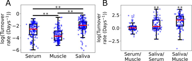
Comparison between tissues for a single subject. (A) All proteins measured in the individual tissues, serum n = 148, muscle n = 156, saliva n = 179. (B) Fold change comparisons for the same protein observed in different tissues. A value of 0 indicates the rate was the same in both tissues. Serum/Muscle n = 80, Saliva/Serum n = 102, Saliva/Muscle n = 80, Significance determined by Tukey–Kramer analysis (** p-value < 0.01).
Comparison of immunoglobulins to other proteins in serum vs saliva was performed using all proteins that were matched between the tissues, with proteins calculated from one or more time points (Figure 9). For single time point comparisons protein turnover rates for day 8 only and day 32 only were matched between saliva and serum and graphed.
Figure 9.
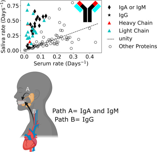
Kinetic data biological significance example. (Top) Rates from serum and saliva were compared showing a large difference in immunoglobin protein turnover rates between tissues. IgA and IgM or unspecified heavy and light chains show larger turnover in saliva than serum. IgG proteins are roughly the same. (Inset) Ig representation. light blue are light chains; red is the heavy chain variable region. (Bottom) This data suggests that IgA and IgM are synthesized in local salivary glands (Path A) while IgG is imported from the circulating blood serum (Path B)
Experimental Design and Statistical rationale
Six human subjects were used (n = 6) to ensure there were sufficient samples for statistical analysis for each gender (3 males and 3 females). Many graphs were log transformed to correct for skew. Comparison graphs used Passing-Bablok tests instead of linear regression, because the Passing-Bablok test is resistant to the outliers often found in biological data.
Results and Discussion
Analysis of Body Water Deuterium Enrichment
In humans the diversity of size, weight, and metabolic rate (Table S1) results in the same deuterium labeling scheme producing varying isotope enrichment curves (Figure 3). Spline fits were calculated as B-splines of a one-dimensional curve, using time and measured deuterium enrichment with each point weighted by three and divided by the standard deviation of the measured deuterium values (Figure 3, dashed black lines). As can be observed in Figure 3, the splines of the enrichment data are resistant to the noise and outliers and were sufficient for the DeuteRater-H analysis. We observed similar spline characteristics for the fit from saliva (subjects S1–S5) or serum (S2, S3, S4, S6). Due to more data being present for saliva, where available, splines from saliva were preferred for all analyses.
Checking for Time Point Bias
Our hypothesis is that a protein sampled at different times in the same subject should provide the same turnover rate. Based on our simulations (Figure S3) the measured deuterium enrichments would result in a wide range of peptides comparable between each time point. To test this, we performed a comparative analysis using only peptide sequences that were present in every time point for a given subject. Our analyses tested whether total enrichment, labeling timespan (Figure 4A and B) or signal intensity (Figure S4) could introduce a bias in the calculated rates with no significant perturbations observed for these variables. Therefore, we can conclude that any observed bias in our results is related to signal-to-noise ratio or a peptide selection bias, not resulting from the calculation method.
To confirm that the constantly increasing deuterium enrichment was enabling us to avoid a time-dependent bias, we did the same analysis using constant label enrichment data from a previously published experiment.8 There was a large and obvious bias for the single point analysis compared to the all time points rates (Figure 4B). Only proteins with rates slow enough to be in the “good” signal-to-noise region (Figure 1D) are able to be analyzed creating a decreasing average for the average protein turnover rate (Figure 4B).
Next, we tested whether individual proteins agreed with the global trends. Matched proteins from each time point were used to prevent selection bias. We then fit the rate calculated with all time points against individual time points using a Passing-Bablok fit (Figure 5). As before, serum data was used since it was the only tissue with more than two time points for which we had data for every subject. Only the slope of time 24 does not contain slope = 1 within its 95% confidence interval, and none of the intercepts were significantly different from 0. Given that a perfectly matched data set would have a slope of 1 and an intercept of 0, this indicates that single time points rates and time points calculated using all time points are not significantly different. If analyzed with paired t tests instead, only the rates calculated using time 32 show any difference from rates calculated using all time points.
In principle it is possible to measure new protein synthesis immediately (within minutes or hours) after providing the isotope.34 Deuterated water distribution and amino acid metabolism are very fast relative to protein synthesis, and in mice amino acid pools are saturated in less than 3 h5 with similar rates in humans.34 Based on the sensitivity of our instruments, we expect that a 10% relative change in the isotope distribution should be accurately quantified. We expect to achieve this minimum signal at earlier times with high n-value peptides in fast turnover proteins in subjects with a faster deuterium ramp (Figure S3). Because of our peptide filtering criteria, this did not significantly reduce the data quality based on the slope and confidence interval of rates in the day 8 sample relative to the use of all time points (Figure 5A). We did observe a nonsignificant increase in the distribution of the fast turnover rate (>0.2 day–1) proteins for the late time single sample analysis (T = 24, 32 days). This could arise from either technical or biological sources. The fact that the spread is almost equally distributed for increases and decreases in rate, suggests that the change is not related to the isotope labeling or calculation methods. These fast turnover proteins will be more responsive to time-dependent regulation and may have a significant dynamic range impacted by diet, activity, or other unmeasured factors.
Comparison to Published Literature
We compared the current results against two published studies6,13 that examined human protein turnover rates in the serum of human subjects using classical enrichment strategies (Figure 6). Statistically significant variation between studies is expected due to differences in locations, subjects, and instrumentation. Therefore, we are testing whether the current nonequilibrium enrichment data is as similar or more similar to the two published data sets as they are to each other. Only proteins shared between all data sets were compared to simplify the analysis, which was performed using Passing-Bablok regressions. This study (DeuteRater-H) vs Ping is not significantly different in slope or intercept, but DeuteRater-H vs Price shows large differences when compared to Ping vs Price. Fortunately, the Price paper provided peptide level turnover rates. When comparing peptide turnover rates instead of proteins (Figure 6D), DeuteRater-H calculated rates are much closer to those reported, though the difference is still significant. This indicates the difference is likely either caused by different peptides being analyzed or a difference in the algorithms used to combine sequence turnover rates into protein turnover rates. A likely cause of a peptide sequence difference is that the Ping lab data were collected on an orbitrap-style instrument similar to this study. While the Price paper data were collected on an Agilent QToF, which often observes a different population of peptides.8 Also, biological details were sparse on the subjects. If for example the Price subjects were on average older than those in the current study, it may introduce real biological differences in protein turnover rate.35
Comparison between Human Subjects
Since humans in the general population vary significantly between each other, we expected significant differences in turnover rates measured between subjects. Comparing the distribution of observed turnover rates in the three measured tissues shows that serum and saliva have no significant differences but muscle has several significant differences (Figure 7). In muscle, S2 has the highest average turnover rates and S3 has the lowest, so it is not surprising that the significant comparisons consistently involved either S2 or S3. S3 was the lowest in all time points, while other subjects varied a bit more. This was not due to gender differences as both S2 and S3 were male, therefore these differences may be due to other factors like exercise routine. For example, if S2 was more active relative to S3, then the S2 turnover rates might be higher due to the need for more protein replacement. Although the testing and dedicated experiments needed to examine the biological significance are outside the scope of this study, this nonequilibrium single-time point methodology would be useful in performing those types of experiments in the future.
Comparison between Different Tissues
We noted that different tissues have different turnover rates even for the same proteins (Figure 8), similar to previous observations.4,5,12 This is expected due to the different roles and conditions experienced by these tissues. For example, saliva is constantly swallowed and so we would expect locally synthesized protein to turnover more rapidly in the saliva than the same protein in the muscle, where proteins support or belong to long-term physiological structures. Indeed, comparisons of proteins that were present in multiple tissues in the same subject (Figure 7) and between subjects (Figure 8A) show that the same protein will generally turnover faster in saliva, and slowest in the muscle, similar to previous observations.4,35
Differing Turnover Rates Based on Synthesis Location
In addition to replicating literature results, maximizing the range of measurable rates in each sample facilitates biological observations. For example, the intertissue comparison in Figure 8 highlights a significant difference in turnover between matched proteins in saliva and other tissues. When examining the types of proteins represented in each group, we discovered that some immunoglobulins exhibited significant tissue-dependent differences in turnover rate, while others did not (Figure 9). Turnover for Immunoglobulin Gamma (IgG) was very similar between tissues (Figure 9 stars). By contrast Immunoglobulin Alpha (IgA) and Immunoglobulin Mu (IgM) were significantly faster in saliva (Figure 9 diamonds), as were any proteins that were not specific to the Immunoglobulin class, such as the light chains. IgA and IgM are both represented by blue diamonds because they are produced in the same location and have similar function. This observation conforms to known saliva biochemistry36 (Figure 9 bottom) where it was previously established37 that salivary IgA and to a lesser extent IgM are produced locally in the salivary glands38 (Figure 9, Path A), separately from their production in the serum.39 In contrast, the similar turnover rate for IgG suggests that it is from a single source for both serum and saliva. This observation also agrees with literature. These results and the literature support a model where IgG in both the serum and saliva is synthesized by circulating immune cells in the blood plasma with active transport from the serum into the saliva (Figure 9B, Path B). We repeated the analysis using single time points at the extremes of the sampling range and saw similar separation between the immunoglobulins (Figure S5).
Conclusion
A full understanding of protein homeostasis (proteostasis, Figure 1A), and its perturbation in related diseases, requires that we observe regulation of synthesis and degradation for each protein in the proteome of individual people. Combining protein quantitation and turnover can provide important new insights into regulation of the proteome in vivo.
Our presented method of nonequilibrium isotope enrichment allows a larger range of turnover rates to be confidently measured from a single sample. In order to facilitate the use of this method by others, we have created the open-source data analysis tool DeuteRater-H, and have herein demonstrated its effectiveness. The program calculates protein turnover rates on a proteome scale. We have enabled the use of spline fits for deuterium enrichment curves to accommodate the variation between human subjects. Comparison to previous studies demonstrates DeuteRater-H’s calculated protein turnover rates are similar to those of previous studies, indicating that our calculation metrics are accurate even with the added complexity required to deal with constantly increasing deuterium enrichment. The source code is freely available, has a user-friendly GUI interface and can simultaneously calculate large numbers of protein turnover rates.
Using these new tools, we were able to reproducibly observe protein turnover up to 0.6 day–1 even in late time points of 32 days, where with a stable enrichment, the fastest rate measurable would be ∼12-fold slower (0.05 day–1). This upper rate limit for our nonequilibrium experiment could in principle be further increased if the deuterium enrichment ramp was faster (Figure 2). In its current form the modified experimental design utilizing a nonequilibrium isotope enrichment extends the range of measurable rates from ∼10-fold to ∼4000-fold in a single muscle biopsy sample. These advantages were observed in a shotgunstyle experiment. The use of targeted experiments with higher sensitivity to isotope incorporation could extend this range significantly34 to access faster and slower turnover rate proteins with the same dosing scheme.
Finally, we demonstrated that turnover analysis can reveal differences in the sources of proteins observed in the same sample (Figure 9). Our data confirmed earlier literature observations that IgG in the saliva is sourced from the blood while IgM and IgA are produced locally. This example of the tissue specific antibody production could, for example, be used to test whether nasal or injection-based vaccination is more effective at creating antigen specific antibodies in different compartments of the body. This general capability could be also useful in studies of cancer, where the sourcing of nutrients from microenvironments can dramatically change health outcomes.
Acknowledgments
This work was supported by a grant from the Fritz B. Burns Foundation to J.C.P.; the National Institutes of Health [R01AG066874] to J.C.P.; Brigham Young University Graduate Research Fellowship to B.C.N.; Brigham Young University Undergraduate Research Awards to C.Q., A.A., A.H., K.J.C., M.H., and D.P.; and National Science Foundation [CHE-1757627] to R.A. DeuteRater running drop in Figure 2 first published in Naylor 2017,8 reproduced with permission.
Supporting Information Available
The Supporting Information is available free of charge at https://pubs.acs.org/doi/10.1021/acs.jproteome.2c00380.
Figure S1: Experimental Design. (Top) Blue rectangles represent different amounts of Deuterium in daily doses, red ovals represent muscle biopsies, red arrows represent blood draws. (Bottom) Simulations of body water deuterium enrichment for a 100 lb (45 kg) subject assuming 40% of the body mass is water replaced at 5% of the volume each day. The simulations suggested that with these doses a heavier person would achieve lower total enrichments but have a similarly linear increase in deuterium. Therefore, a single dosing pattern was used for all subjects. Figure S2: For subjects where 2H2O was measured in both saliva and serum, splines (black dashed lines) were calculated for each. Red dots are saliva measurements, blue diamonds are serum measurements. Figure S3: Time required for measurable changes in isotope distributions were simulated for an expected range of peptide turnover rates (k, 0.05–1.5), incorporated number of deuteriums (n-value, 6–40) at different body water deuterium enrichments (1, 2, or 3% final enrichments). The same data is displayed as 3D surface (Top) with time on the z-axis or a contour map with the time from 1 to 100 days displayed as a color gradient from dark blue (1 day) to red and white (90–100). The minimum time to detectability is expected to be after 9.0 days for a 1% ramp, 5.0 days for a 2% ramp, and 3.5 days for a 3% ramp for peptides with the largest rate (k) and n-value. Figure S4: Measurements of serum albumin peptides (SA) were used to explore whether signal intensity introduces any bias in the calculation of kinetic rates. Since SA is the most abundant protein in the serum, we had ∼2300 measured peptide rates across the entire range of signal intensity. Although low signal intensity peptides are more frequently filtered out by the quality filters, there was no statistical support for a signal intensity bias on rate. Figure S5: Comparison of serum and saliva turnover rates with a focus on immunoglobulins. Only single time points were used. Panel A only uses rates calculated from 8-day samples, Panel B only uses rates calculated from 32-day samples. This demonstrates that the individual time points at the extreme ends of the experiment still show the biologically relevant pattern that IgA and IgM are produced in the saliva and serum separately with separate turnover rates (PDF)
Supplemental Table S1 – Data about subjects in this study. Supplemental Table S2 – Every protein observed in this study. Columns are rates for different subjects calculated from either calculating the average or median of all calculated peptide sequence rates. Supplemental Table S3 – Summary of peptide sequence rates from serum using all time points or only one or two time points. Columns indicate if the all calculated peptide sequence rates that passed DeuteRater-H’s filters (all) or only those peptide sequences that passed DeuteRater-H’s filters and were present in all time points (matched). Supplemental Table S4 – Serum data for every protein observed, for every condition used in the paper. Average rates and standard deviations are provided for all single time points and combinations. Combinations are indicated by a certain number of time points (t) being required, and are labeled as require_t_time points. Supplemental Table S5 – Muscle data for every protein observed, for every condition used in the paper. Average rates and standard deviations are provided for all single time points and combinations. Combinations are indicated by a certain number of time points (t) being required, and are labeled as require_t_time points. Supplemental Table S6 – Saliva data for every protein observed, for every condition used in the paper. Average rates and standard deviations are provided for all single time points and combinations. Combinations are indicated by a certain number of time points (t) being required, and are labeled as require_t_time points. Supplemental Table S7 – Serum data for every peptide sequence observed, for every condition used in the paper. Calculated rates and mean of all absolute residuals are provided for all single time points and combinations. Combinations are indicated by a certain number of time points (t) being required, and are labeled as require_t_time points. Supplemental Table S8 – Muscle data for every peptide sequence observed, for every condition used in the paper. Calculated rates and mean of all absolute residuals are provided for all single time points and combinations. Combinations are indicated by a certain number of time points (t) being required, and are labeled as require_t_time points. Supplemental Table S9 – Saliva data for every peptide sequence observed, for every condition used in the paper. Calculated rates and mean of all absolute residuals are provided for all single time points and combinations. Combinations are indicated by a certain number of time points (t) being required, and are labeled as require_t_time points. Supplemental Table S10 – Data from mice labeled with a constant enrichment strategy and bolus injection for the purpose of comparing flat vs rising enrichment schemes. Shown in Figure 4C. “Accession” is the Uniprot accession number. “Protein Name” is the common name of the protein. The “all data 3 timepoints required” allowed the calculation software to use any available time points, but required at least 3 different time points to calculate a rate. The “day 8 turnover rate” indicates rates calculated using time 8 days only. The “day 32 turnover rate” indicates rates calculated using time 32 days only. Blank cells indicate a protein was not observed at the relevant time, or there were enough errors with the measurement that the rate was filtered out. Supplemental Table S11 – Amino acid specific physical constants used in the DeuteRater algorithm (XLSX)
The authors declare no competing financial interest.
Notes
Raw Data:https://chorusproject.org/pages/index.html project number 1741. DeuteRater-H Source Code: https://github.com/JC-Price/DeuteRater-H. DeuteRater-H exe: https://github.com/JC-Price/DeuteRater-H/releases/tag/v1.0.
Supplementary Material
References
- Pulk A.; Liiv A.; Peil L.; Maivali U.; Nierhaus K.; Remme J. Ribosome reactivation by replacement of damaged proteins. Molecular microbiology 2010, 75 (4), 801–814. 10.1111/j.1365-2958.2009.07002.x. [DOI] [PubMed] [Google Scholar]
- Sinturel F.; Gerber A.; Mauvoisin D.; Wang J.; Gatfield D.; Stubblefield J. J.; Green C. B.; Gachon F.; Schibler U. Diurnal Oscillations in Liver Mass and Cell Size Accompany Ribosome Assembly Cycles. Cell 2017, 169 (4), 651–663. 10.1016/j.cell.2017.04.015. [DOI] [PMC free article] [PubMed] [Google Scholar]
- Ma X. M.; Blenis J. Molecular mechanisms of mTOR-mediated translational control. Nat. Rev. Mol. Cell Biol. 2009, 10 (5), 307–318. 10.1038/nrm2672. [DOI] [PubMed] [Google Scholar]
- Price J.; Guan S.; Burlingame A.; Prusiner S.; Ghaemmaghami S. Analysis of proteome dynamics in the mouse brain. Proc. Natl. Acad. Sci. U.S.A. 2010, 107 (32), 14508–14513. 10.1073/pnas.1006551107. [DOI] [PMC free article] [PubMed] [Google Scholar]
- Price J.; Khambatta C.; Li K.; Bruss M.; Shankaran M.; Dalidd M.; Floreani N.; Roberts L.; Turner S.; Holmes W.; et al. The Effect of Long Term Calorie Restriction on in Vivo Hepatic Proteostatis: A Novel Combination of Dynamic and Quantitative Proteomics. Molecular & Cellular Proteomics 2012, 11 (12), 1801–1814. 10.1074/mcp.M112.021204. [DOI] [PMC free article] [PubMed] [Google Scholar]
- Price J. C.; Holmes W. E.; Li K. W.; Floreani N. A.; Neese R. A.; Turner S. M.; Hellerstein M. K. Measurement of human plasma proteome dynamics with (2)H(2)O and liquid chromatography tandem mass spectrometry. Anal. Biochem. 2012, 420 (1), 73–83. 10.1016/j.ab.2011.09.007. [DOI] [PubMed] [Google Scholar]
- Shankaran M.; King C. L.; Angel T. E.; Holmes W. E.; Li K. W.; Colangelo M.; Price J. C.; Turner S. M.; Bell C.; Hamilton K. L.; et al. Circulating protein synthesis rates reveal skeletal muscle proteome dynamics. J. Clin Invest 2016, 126 (1), 288–302. 10.1172/JCI79639. [DOI] [PMC free article] [PubMed] [Google Scholar]
- Naylor B. C.; Porter M. T.; Wilson E.; Herring A.; Lofthouse S.; Hannemann A.; Piccolo S. R.; Rockwood A. L.; Price J. C. DeuteRater: a tool for quantifying peptide isotope precision and kinetic proteomics. Bioinformatics 2017, 33 (10), 1514–1520. 10.1093/bioinformatics/btx009. [DOI] [PubMed] [Google Scholar]
- Mathis A. D.; Naylor B. C.; Carson R. H.; Evans E.; Harwell J.; Knecht J.; Hexem E.; Peelor F. F.; Miller B. F.; Hamilton K. L.; et al. Mechanisms of In Vivo Ribosome Maintenance Change in Response to Nutrient Signals. Mol. Cell Proteomics 2017, 16 (2), 243–254. 10.1074/mcp.M116.063255. [DOI] [PMC free article] [PubMed] [Google Scholar]
- Decaris M. L.; Emson C. L.; Li K.; Gatmaitan M.; Luo F.; Cattin J.; Nakamura C.; Holmes W. E.; Angel T. E.; Peters M. G.; et al. Turnover rates of hepatic collagen and circulating collagen-associated proteins in humans with chronic liver disease. PLoS One 2015, 10 (4), e0123311 10.1371/journal.pone.0123311. [DOI] [PMC free article] [PubMed] [Google Scholar]
- Decaris M. L.; Li K. W.; Emson C. L.; Gatmaitan M.; Liu S.; Wang Y.; Nyangau E.; Colangelo M.; Angel T. E.; Beysen C.; et al. Identifying nonalcoholic fatty liver disease patients with active fibrosis by measuring extracellular matrix remodeling rates in tissue and blood. Hepatology 2017, 65 (1), 78–88. 10.1002/hep.28860. [DOI] [PMC free article] [PubMed] [Google Scholar]
- Lam M. P.; Wang D.; Lau E.; Liem D. A.; Kim A. K.; Ng D. C.; Liang X.; Bleakley B. J.; Liu C.; Tabaraki J. D.; et al. Protein kinetic signatures of the remodeling heart following isoproterenol stimulation. J. Clin Invest 2014, 124 (4), 1734–1744. 10.1172/JCI73787. [DOI] [PMC free article] [PubMed] [Google Scholar]
- Wang D.; Liem D. A.; Lau E.; Ng D. C.; Bleakley B. J.; Cadeiras M.; Deng M. C.; Lam M. P.; Ping P. Characterization of human plasma proteome dynamics using deuterium oxide. Proteomics Clin Appl. 2014, 8 (7–8), 610–619. 10.1002/prca.201400038. [DOI] [PMC free article] [PubMed] [Google Scholar]
- Previs S. F.; Fatica R.; Chandramouli V.; Alexander J. C.; Brunengraber H.; Landau B. R. Quantifying rates of protein synthesis in humans by use of 2H2O: application to patients with end-stage renal disease. Am. J. Physiol Endocrinol Metab 2004, 286 (4), E665–672. 10.1152/ajpendo.00271.2003. [DOI] [PubMed] [Google Scholar]
- Hsieh E. J.; Shulman N. J.; Dai D. F.; Vincow E. S.; Karunadharma P. P.; Pallanck L.; Rabinovitch P. S.; MacCoss M. J. Topograph, a software platform for precursor enrichment corrected global protein turnover measurements. Mol. Cell Proteomics 2012, 11 (11), 1468–1474. 10.1074/mcp.O112.017699. [DOI] [PMC free article] [PubMed] [Google Scholar]
- Basak J. M.; Kim J.; Pyatkivskyy Y.; Wildsmith K. R.; Jiang H.; Parsadanian M.; Patterson B. W.; Bateman R. J.; Holtzman D. M. Measurement of apolipoprotein E and amyloid beta clearance rates in the mouse brain using bolus stable isotope labeling. Mol. Neurodegener 2012, 7, 14. 10.1186/1750-1326-7-14. [DOI] [PMC free article] [PubMed] [Google Scholar]
- Hammond D. E.; Simpson D. M.; Franco C.; Wright Muelas M.; Waters J.; Ludwig R. W.; Prescott M. C.; Hurst J. L.; Beynon R. J.; Lau E. Harmonizing Labeling and Analytical Strategies to Obtain Protein Turnover Rates in Intact Adult Animals. Mol. Cell Proteomics 2022, 21 (7), 100252. 10.1016/j.mcpro.2022.100252. [DOI] [PMC free article] [PubMed] [Google Scholar]
- Smith R.; Taylor R. M.; Prince J. T. Current controlled vocabularies are insufficient to uniquely map molecular entities to mass spectrometry signal. BMC Bioinformatics 2015, 16 (S7), S2. 10.1186/1471-2105-16-S7-S2. [DOI] [PMC free article] [PubMed] [Google Scholar]
- Kasumov T.; Ilchenko S.; Li L.; Rachdaoui N.; Sadygov R. G.; Willard B.; McCullough A. J.; Previs S. Measuring protein synthesis using metabolic 2H labeling, high-resolution mass spectrometry, and an algorithm. Anal. Biochem. 2011, 412 (1), 47–55. 10.1016/j.ab.2011.01.021. [DOI] [PMC free article] [PubMed] [Google Scholar]
- Hellerstein M. K. Relationship between precursor enrichment and ratio of excess M2/excess M1 isotopomer frequencies in a secreted polymer. J. Biol. Chem. 1991, 266 (17), 10920–10924. 10.1016/S0021-9258(18)99107-6. [DOI] [PubMed] [Google Scholar]
- Guan S.; Price J. C.; Ghaemmaghami S.; Prusiner S. B.; Burlingame A. L. Compartment modeling for mammalian protein turnover studies by stable isotope metabolic labeling. Anal. Chem. 2012, 84 (9), 4014–4021. 10.1021/ac203330z. [DOI] [PMC free article] [PubMed] [Google Scholar]
- Peronnet F.; Mignault D.; du Souich P.; Vergne S.; Le Bellego L.; Jimenez L.; Rabasa-Lhoret R. Pharmacokinetic analysis of absorption, distribution and disappearance of ingested water labeled with D(2)O in humans. Eur. J. Appl. Physiol 2012, 112 (6), 2213–2222. 10.1007/s00421-011-2194-7. [DOI] [PMC free article] [PubMed] [Google Scholar]
- Katz J. J. Chemical and Biological Studies with Deuterium. Am. Sci. 1960, 48 (4), 544–580. [Google Scholar]
- Money K. E.; Myles W. S. Heavy water nystagmus and effects of alcohol. Nature 1974, 247 (5440), 404–405. 10.1038/247404a0. [DOI] [PubMed] [Google Scholar]
- Ganusov V. V.; Borghans J. A.; De Boer R. J. Explicit kinetic heterogeneity: mathematical models for interpretation of deuterium labeling of heterogeneous cell populations. PLoS Comput. Biol. 2010, 6 (2), e1000666 10.1371/journal.pcbi.1000666. [DOI] [PMC free article] [PubMed] [Google Scholar]
- Lis G.; Wassenaar L. I.; Hendry M. J. High-precision laser spectroscopy D/H and 18O/16O measurements of microliter natural water samples. Anal. Chem. 2008, 80 (1), 287–293. 10.1021/ac701716q. [DOI] [PubMed] [Google Scholar]
- Abbott C. B.; Lawrence M. M.; Kobak K. A.; Lopes E. B. P.; Peelor F. F. 3rd; Donald E. J.; Van Remmen H.; Griffin T. M.; Miller B. F. A Novel Stable Isotope Approach Demonstrates Surprising Degree of Age-Related Decline in Skeletal Muscle Collagen Proteostasis. Function (Oxf) 2021, 2 (4), zqab028. 10.1093/function/zqab028. [DOI] [PMC free article] [PubMed] [Google Scholar]
- Zhang J.; Xin L.; Shan B.; Chen W.; Xie M.; Yuen D.; Zhang W.; Zhang Z.; Lajoie G. A.; Ma B. PEAKS DB: de novo sequencing assisted database search for sensitive and accurate peptide identification. Mol. Cell Proteomics 2012, 11 (4), M111.010587. 10.1074/mcp.M111.010587. [DOI] [PMC free article] [PubMed] [Google Scholar]
- Rockwood A. L.; Haimi P. Efficient calculation of accurate masses of isotopic peaks. J. Am. Soc. Mass Spectrom. 2006, 17 (3), 415–419. 10.1016/j.jasms.2005.12.001. [DOI] [PubMed] [Google Scholar]
- Virtanen P.; Gommers R.; Oliphant T. E.; Haberland M.; Reddy T.; Cournapeau D.; Burovski E.; Peterson P.; Weckesser W.; Bright J.; van der Walt S. J.; Brett M.; Wilson J.; Millman K. J.; Mayorov N.; Nelson A. R. J.; Jones E.; Kern R.; Larson E.; Carey C J; Polat I.; Feng Y.; Moore E. W.; VanderPlas J.; Laxalde D.; Perktold J.; Cimrman R.; Henriksen I.; Quintero E. A.; Harris C. R.; Archibald A. M.; Ribeiro A. H.; Pedregosa F.; van Mulbregt P.; SciPy 1.0 Contributors SciPy 1.0: Fundamental Algorithms for Scientific Computing in Python. Nat. Methods 2020, 17 (3), 261–272. 10.1038/s41592-019-0686-2. [DOI] [PMC free article] [PubMed] [Google Scholar]
- Hindmarsh A. C.ODEPACK: Ordinary differential equation solver library; The SAO/NASA Astrophysics Data System, 2019. [Google Scholar]
- Press W. H. T.; Saul A.; Vetterling; William T.; Flannery; Brian P.. Numerical Recipes: The Art of Scientific Computing; Cambridge University Press, 2007. [Google Scholar]
- SAS Institute. JMP; SAS Institute Inc.: Cary, NC, 2021.
- Wilkinson D. J.; Cegielski J.; Phillips B. E.; Boereboom C.; Lund J. N.; Atherton P. J.; Smith K. Internal comparison between deuterium oxide (D2O) and L-[ring-13C6] phenylalanine for acute measurement of muscle protein synthesis in humans. Physiol. Rep. 2015, 3 (7), e12433. 10.14814/phy2.12433. [DOI] [PMC free article] [PubMed] [Google Scholar]
- Karunadharma P. P.; Basisty N.; Dai D. F.; Chiao Y. A.; Quarles E. K.; Hsieh E. J.; Crispin D.; Bielas J. H.; Ericson N. G.; Beyer R. P.; et al. Subacute calorie restriction and rapamycin discordantly alter mouse liver proteome homeostasis and reverse aging effects. Aging Cell 2015, 14 (4), 547–557. 10.1111/acel.12317. [DOI] [PMC free article] [PubMed] [Google Scholar]
- Brandtzaeg P. Human secretory immunoglobulin M., An immunochemical and immunohistochemical study. Immunology 1975, 29 (3), 559–570. [PMC free article] [PubMed] [Google Scholar]
- Korsrud F. R.; Brandtzaeg P. Quantitative immunohistochemistry of immunoglobulin- and J-chain-producing cells in human parotid and submandibular salivary glands. Immunology 1980, 39 (2), 129–140. [PMC free article] [PubMed] [Google Scholar]
- Strober W.; Blaese R. M.; Waldmann T. A. The origin of salivary IgA. J. Lab Clin Med. 1970, 75 (5), 856–862. [PubMed] [Google Scholar]
- Brandtzaeg P. Human secretory immunoglobulins. II., Salivary secretions from individuals with selectively excessive or defective synthesis of serum immunoglobulins. Clin. Exp. Immunol. 1971, 8 (1), 69–85. [PMC free article] [PubMed] [Google Scholar]
Associated Data
This section collects any data citations, data availability statements, or supplementary materials included in this article.