Abstract
This article is dedicated analyzing the interdependence of oil prices and exchange rate movements of oil exporting countries (the Russian ruble, Euro, Canadian dollar, Chinese yuan, Brazil real, Nigerian naira, Algerian dinar). The study also considers risk-based oil market spillovers in global crisis periods with integrated decision recommendation systems. For this purpose, a fuzzy decision-making model is created by considering the bipolar model and imputation of expert evaluations with collaborative filtering. The main contribution of this study is both its econometric analysis and evaluations based on expert opinions. This helps reach more crucial results. All three of the recent shocks (2008, 2012, 2020) in the oil market are transmitted to foreign exchange markets of oil-producing countries. At the same time, the last shock of 2020 caused by the COVID-19 pandemic has not yet been fully reflected on the Russian ruble exchange rate. Correlation parameters became weaker in the last year, as the Russian ruble correlation coefficient fluctuates between − 0.5 and 0.5. However, before 2020 the spillover effect had a higher significance (in the range from − 0.8 to − 0.1). Nigerian naira and Algerian dinar were showing almost the same movements, while the Russian Ruble was in a different trading range.
Keywords: Analytics, Bipolar QROFSs, Golden cut, M-SWARA, ELECTRE
Introduction
The spillover effect on currency exchange rates in oil exporting countries changed after the pandemic-induced financial crisis beginning in 2020. The novelty of this study is the relationship between oil price market volatility and exchange rate movements of oil exporting countries. This paper proves the idea that the spillover effect in Algeria, Nigeria, and Russia became weaker after the beginning of the pandemic-related crisis. The choice of oil exporting countries is motivated by academic studies about the interdependence between the oil prices dynamics and exchange rate movements (Al-Awadhi et al., 2020; Altig et al., 2020).
This article builds on the ideas described in previous works (Mikhaylov, 2018; Norouzi et al., 2020; Ramelli & Wagner, 2020; Salisu & Akanni, 2020). During the studied period, the zero-coupon yield curve of oil exporting countries flattened, acquiring a positive slope inherent to a "healthy" economy. Prolonged increases in labor productivity reduce real marginal costs over a long period of time and lead to lower inflation. In general, the model of endogenous growth in oil consumption and inflation has already been described in sufficient detail.
The motivation for choosing the topic of interdependence between oil prices dynamics and exchange rate movements is based on previous research papers (Norouzi et al., 2020; Ramelli & Wagner, 2020; Salisu & Akanni, 2020).
The theoretical basis for addressing the topic of interdependence between the oil prices dynamics and exchange rate movements is the literature review fundamentals (Szczygielski et al., 2021; Wen et al., 2021). Recent studies show that the spillover effect on currency exchange rates in oil exporting countries responds to innovation process, economic growth and energy markets (Mazur et al., 2021; Narayan, 2020; Nguyen et al., 2021).
The research paper makes contributions to the growing literature about the effects of COVID-19 on the spillover effect on currency exchange rates int oil exporting countries (Fang et al., 2021; Szczygielski et al., 2021; Wen et al., 2021). Recent studies have shown how the spillover effect has changed in oil exporting countries. Moreover, another evaluation is also performed regarding risk-based oil market spillovers in global crisis periods with integrated decision recommendation systems. For this purpose, a fuzzy decision-making model is created by considering bipolar q-ROFSs (Q-Rung Orthopair Fuzzy Sets), M-SWARA (Step-wise Weight Assessment Ratio Analysis), ELECTRE (ÉLimination Et Choix Traduisant la REalité) and imputation of expert evaluations with collaborative filtering (Bhuiyan et al., 2022; Keršuliene et al., 2010). Another important contribution of this study is to make both econometric analysis and evaluations based on expert opinions. This helps reach more effective results.
This study argues that the exchange rate variability has an asymmetric effect on international trade flows. The study of Bahmani-Oskooee and Aftab (2017) shows that prices of trade goods respond to volatility of the exchange rate in an asymmetric manner. Additionally, exchange rate volatility affects trade flows in an asymmetric manner in both the short- and long-term (Bahmani-Oskooee & Aftab, 2017). Therefore, this study argues that exchange rate volatility responds to trade flows of both imports and exports in an asymmetric manner. The exchange rate is the topic of interest for many researchers particularly in developing countries as it bridges a country with the rest of the world, as it determines the relative prices and competitive position of a country in the international market (Aliyu, 2010). The topic of exchange rates is a prime interest for those countries that shifted their policy from fix to floating exchange rate systems.
These studies use methods such as least squares regression, panel regression or simple co-integration. Furthermore, almost all studies conducted assumed that oil prices affect exchange rate volatility symmetrically. Although recently Bahmani-Oskooee and Aftab (2017) propose that prices of trade goods and trade flow respond to volatility of exchange rates in an asymmetric manner.
Literature Review
Exchange rate volatility is defined as the persistent fluctuations of exchange rates garnered broader attention in recent studies due to its major effect on developing economies. Developing economies interact with developed countries, and are consequentially confronted with volatility on their foreign exchange markets and its subsequent impact on exports and the state’s trade balance (Bahmani-Oskooee & Wang, 2007), volume of country investments, growth of employment in country, growth of inflation, output growth rate, international trade and more macroeconomic indicators, specifically those evaluating the economic activity in the country.
The available literature on exchange rate volatility and oil prices does not provide clear conclusions on whether the impact of exchange rate volatility is positive, negative or both. Many studies examine the short-, intermediate-, and long-term volatility spillovers between developed (Australia, Canada, France, Germany, Japan, UK, and US) and emerging BRICS (Brazil, Russia, China, India, and South Africa) stock markets and strategic oil futures markets.
In the empirical findings of previous studies, the net effect of oil prices on exchange rate volatility is inconsistent. Thirdly, there is no link in exchange rate volatility and oil prices. Thus, the association of exchange rate volatility of oil exporting countries and oil prices is still inconclusive. There are many reasons for this inconsistency in literature.
Theoretically, the inconclusiveness is due to the different attitude regarding risk that international traders have. Some are risk-averse while some are risk-loving. Risk-averse traders substitute international trade with domestic trade to avoid exchange rate volatility. While risk-loving investors increase international trade to earn more profit as compensation in case of favorable effects of exchange rate volatility on trade flows. The higher volatility of exchange rates creates higher profit opportunities for risk-neutral investors during corresponding periods in the market. Forward markets reduce the volatility’s influence but do not make markets more affordable or attractive to small firms. Empirically, some recent studies conclude that the indeterminate results of past studies are due to the over-reliance on aggregated trade flows and weak econometric techniques.
The effect of exchange rate volatility at the industry level is studied (Dutta, 2018; Jammazi et al., 2017; Ji et al., 2018). The authors find that the correlation is different from industry to industry and does not show unidirectional impact. After the mixed findings of previous studies, the effect of exchange rate volatility on trade is neither entirely significant nor completely unidirectional. It differs for the horizon of study and the market of interest, thus requiring more disaggregated trade data for future research.
The relationship between exchange rate volatility and oil prices volatility among nations has been studied through various approaches empirically. The existing literature falls into any of the following strands. Firstly, earlier studies applied aggregated trade data of a country to the remaining world. The results of these studies are mixed. Secondly, due to the problems of aggregation bias, later studies disaggregate data at the bilateral level. The second flow of recent studies took imports and exports separately to overcome the problem of aggregation bias: these studies disaggregate data not only at a country level but also at the industry level and in some cases even at the product level.
Multi-scale risk connectedness between economic policy uncertainty of China and global oil prices in time–frequency domains discussed the connection between exchange rate and oil price (Cheng et al., 2022; Wang & Lee, 2020; Wei, 2019).
From an econometric aspect, previous studies used various analysis techniques that recent research concluded to be inappropriate. These studies used methods that do not account for mixed integration cases. It is a known norm in the trade demand model that exchange rate volatility follows the stationary level I (0). The above-discussed issues lead to inappropriate discussions and misleading policy recommendations.
Due to mixed and inappropriate findings of previous studies, research papers used disaggregated trade data for each trading partner and industry level to conclude more accurate results and policy recommendations for each trading partner and industry. An interesting research paper in the panel framework compared the effects of exchange rate volatility on international trade flows of developed and developing countries. The study concludes that exports of developing economies are more sensitive to the volatility of the exchange rate. More precisely studies (Norouzi et al., 2020; Ramelli & Wagner, 2020; Salisu & Akanni, 2020) concentrate on ASEAN and conclude that exchange rate volatility results in the decline of international trade flows.
The main hypothesis is that the significant spillover effect between Brent oil prices and currency rates, key values of the F-test and p-value exists between 12 different national currencies of main oil exporting countries: Saudi Arabian Riyal, Iraqi dinar, UAE dirham, Kuwaiti dinar, Iranian dinar, Algerian Dinar, Nigerian Naira, Russian Ruble, US dollar, Canadian dollar, Chinese yuan, Brazil real and Brent Oil prices for the period from 2001 to 2021 (Mazur et al., 2021; Narayan, 2020; Nguyen et al., 2021).
Methods
This section defines the VAR methodology, bipolar q-ROFSs, M-SWARA, ELECTRE and imputation of expert evaluations with collaborative filtering.
VAR Methodology
The paper uses data from Thomson Reuters on 12 different national currencies of main oil exporting countries: Saudi Arabian Riyal, Iraqi dinar, UAE dirham, Kuwaiti dinar, Iranian dinar, Algerian Dinar, Nigerian Naira, Russian Ruble, US dollar, Canadian dollar, Chinese yuan, Brazil real. Moreover, the research paper examines Brent Oil prices for the period from 2001 to 2021. For further analysis, the paper uses daily returns with the 1-step rolling window correlation coefficient. Like in previous research, the length of rolling window is about 36 months (Szczygielski et al., 2021; Wen et al., 2021). Table 1 shows top oil producing countries. Most of OPEC (Organization of the Petroleum Exporting Countries) do not have a free-floating national currency, specifically: Saudi Arabian Riyal, Iraqi dinar, UAE dirham, Kuwaiti dinar, Iranian dinar. These currencies link to USD. Therefore, the paper does not include these currencies into analyses.
Table 1.
Top oil producing countries (OPEC and Non-OPEC)
| Rank | Country | November, 2020 (million barrels per day) |
|---|---|---|
| Top 7 Producing Countries (OPEC) | ||
| 1 | Saudi Arabia | 9.01 |
| 2 | Iraq | 3.82 |
| 3 | United Arab Emirates | 2.51 |
| 4 | Kuwait | 2.30 |
| 5 | Iran | 1.90 |
| 6 | Nigeria | 1.44 |
| 7 | Algeria | 0.87 |
| Total Top 5 OPEC production | 19.54 | |
| Total OPEC production | 29.97 | |
| Top 5 Producing Countries (Non-OPEC) | ||
| 1 | U.S. (50 States) | 18.40 |
| 2 | Russia | 10.24 |
| 3 | Canada | 5.46 |
| 4 | China | 5.00 |
| 5 | Brazil | 3.93 |
| Total Top 5 Non-OPEC production | 43.03 | |
| Total Non-OPEC production | 63.47 | |
Source Author calculation, Thomson Reuters
The paper uses several methods for analyzing correlation and regression in order to investigate the spillover effect between oil prices and foreign exchange rates of national currencies (Russian Ruble, EURUSD, Canadian dollar, Chinese yuan, Brazil real, Nigerian naira, Algerian dinar as large oil exporters). Pearson correlation coefficients and linear regression models are the most suitable for this purpose. Many previous articles used the determination coefficient:
| 1 |
Moreover, the analysis includes F-statistics for linear regression equations and its significance:
| 2 |
Many authors used the t-test for Pearson correlation for such data:
| 3 |
where is the total sum of squares, is the sum of squared residuals, is the explained sum of squares, is the number of observations, is the number of explanatory variables, is the correlation coefficient for this data, is the level of significance.
The study also conducts the Daily Returns Analysis of Currency rates in the data set. After this the paper uses the linear regression model for as follows:
| 4 |
where is the column-vector parameter:
| 5 |
| 6 |
The data sample consists of two groups , , and corresponding parameters such as , , . The VAR model can be used for testing two alternative hypotheses:
| 7 |
There are many statistics, which are subject to F distribution:
| 8 |
The VAR model is used to find the linear interdependencies among many time series. The current paper implements the VAR model for finding the mean spillover between Brent oil prices and national currencies’ volatilities. This is the bivariate VAR model for Brent oil volatility and national currencies’ rates (Russian Ruble, EURUSD, Canadian dollar, Chinese yuan, Brazil real, Nigerian naira, and Algerian dinar):
| 9 |
| 10 |
where are the logarithmic returns of Brent oil volatility and national currencies’ rates (Russian Ruble, EURUSD, Canadian dollar, Chinese yuan, Brazil real, Nigerian naira, and Algerian dinar), μo and μv are the respective conditional mean series. The lag orders are m and n with maximum lag values of M and N. Mean spillover coefficients are for the fx market rates. are the for across fx rates. are the parameters of residual series for the VAR model. This VAR model make the basis for volatility spillover effect calculations.
Bipolar q-ROFSs with Golden Cut
ATANASSOV (1999) generated IFSs by defining membership and non-membership degrees (MED, NED). The details of these sets and requirements are shown in Eqs. (11) and (12) where ( represent the degrees.
| 11 |
| 12 |
PFSs are introduced by Yager (2013) by new degrees (. The details are shown in Eqs. (13) and (14).
| 13 |
| 14 |
Yager (2016) produced q-ROFSs by generalizing IFSs and PFSs. Equations (15) and (16) include the details of these sets.
| 15 |
| 16 |
Zhang (1994) developed bipolar fuzzy sets to cope with uncertainty problems better. They are detailed in Eq. (17) in which shows the satisfaction degree and indicates the satisfaction of the same element.
| 17 |
Equations (18)-(23) include the adoption of these sets to PFSs, IFSs and q-ROFSs.
| 18 |
| 19 |
| 20 |
| 21 |
| 22 |
| 23 |
They are detailed in Fig. 1.
Fig. 1.
Degrees of bipolar IFS, PFS, and q-ROFSs
The sum and product of IFSs can be calculated by computing methods of their differences and quotients. The product of lambda and B tends to 0, as lambda converge to 0 no matter what the value of B is.
Equations (24)–(26) are used for defuzzification.
| 24 |
| 25 |
| 26 |
The Golden cut ( is considered in this study to compute the weights (Belluscio et al., 2021). Equations (27)-(29) represent the details.
| 27 |
| 28 |
| 29 |
Equations (30)–(32) include the integration of this ratio to bipolar fuzzy sets.
| 30 |
| 31 |
| 32 |
M-SWARA method with bipolar q-ROFSs
KERšULIENE et al. (2010) introduced SWARA to weight the factors. With the help of expert evaluations, relation matrix is given in Eq. (33).
| 33 |
Bipolar q-ROFSs are created, and the score functions are calculated in the next step. Equations (34)–(36) are considered to compute key determinants where represents the coefficient value, shows the recalculated weight, explains the comparative importance rate and demonstrates the weights of the criteria.
| 34 |
| 35 |
;
| 36 |
Finally, owing to limitation and transposing the matrix by the power of 2t + 1, the weights are computed.
ELECTRE with Bipolar q-ROFSs
BENAYOUN et al. (1966) introduced ELECTRE with the purpose of ranking the alternatives. Expert evaluations are considered to generate the decision matrix and are calculated as presented in Eq. (37).
| 37 |
Equation (38) is used for normalization.
| 38 |
Weights are computed by Eq. (39).
| 39 |
Equations (40)–(45) represent concordance and discordance (C and D) interval matrixes.
| 40 |
| 41 |
| 42 |
| 43 |
| 44 |
| 45 |
Equations (46)–(53) are used for the creation of the concordance E, discordance F and aggregated G index matrices.
| 46 |
| 47 |
| 48 |
| 49 |
| 50 |
| 51 |
| 52 |
| 53 |
The sets of concordance, discordance and aggregated index matrixes are demonstrated by , , . Also, and indicate the significant items. Net superior , inferior , and overall values are also defined in Eqs. (54)–(56).
| 54 |
| 55 |
| 56 |
Imputation of Expert Evaluations with Collaborative Filtering
Collaborative filtering is considered with the purpose of making predictions for missing evaluations. Because the experts may not have sufficient knowledge to evaluate all items, some can be missing. This methodology helps solve this problem (Liu & Lee, 2010). Equation (57) indicates the details.
| 57 |
In this equation, refers to the similarity index whereas and demonstrate the rating degrees. Additionally, and indicate the averaged values. Prediction index is shown in Eq. (58).
| 58 |
Results
Analysis of Daily Returns in Brent Oil Prices and National Currencies Rates with VAR
Also, the model includes the analysis of daily returns between oil prices and national currency exchange rates to USD fluctuations for the period from 2001 to 2021 on the daily timeframe. It shows the tendency before the global financial crisis of 2008 as well (Figs. 2, 3, 4, 5, 6, 7, 8 and 9).
Fig. 2.
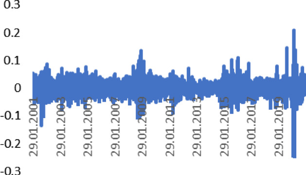
Daily Returns of Brent Oil prices (2001–2021). Source Author calculation, Thomson Reuters
Fig. 3.
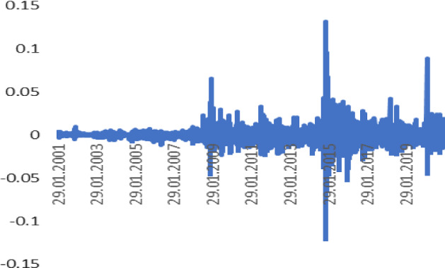
Daily Returns of RUB/USD rate (2001–2021). Source Author calculation, Thomson Reuters
Fig. 4.
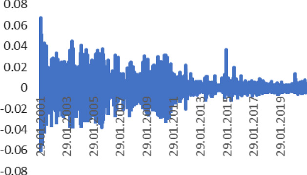
Daily Returns of DZD/USD rate (2001–2021). Source Author calculation, Thomson Reuters
Fig. 5.
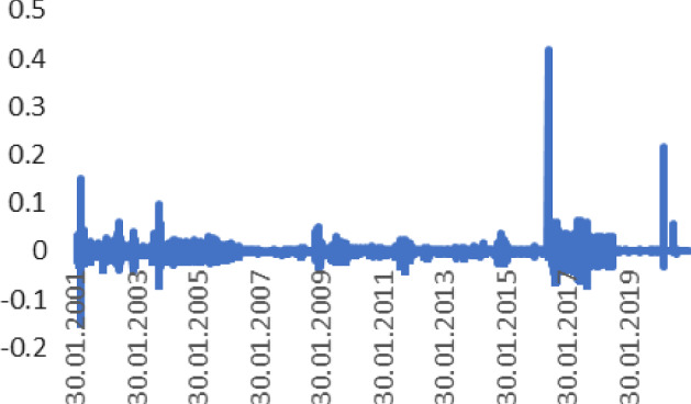
Daily Returns of NGN/USD (2001–2021). Source Author calculation, Thomson Reuters
Fig. 6.
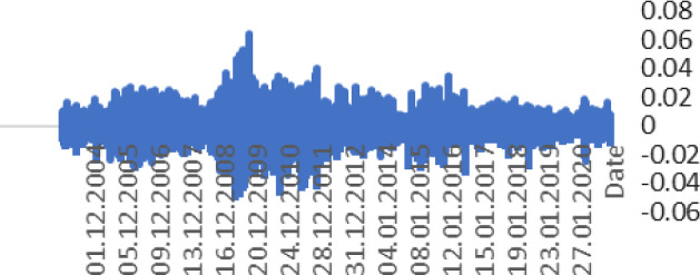
Daily Returns of EUR/USD (2001–2021). Source Author calculation, Thomson Reuters
Fig. 7.
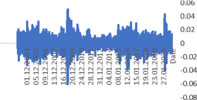
Daily Returns of CAD/USD (2001–2021). Source Author calculation, Thomson Reuters
Fig. 8.
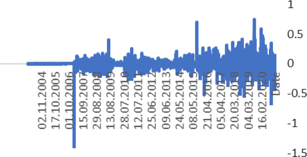
Daily Returns of CNY/USD (2001–2021). Source Author calculation, Thomson Reuters
Fig. 9.
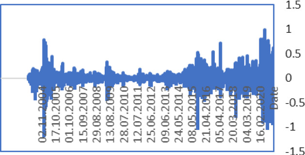
Daily Returns of BRL/USD (2001–2021). Source Author calculation, Thomson Reuters
In the result of graphical analysis of daily returns, the spillover effect between the variables shows the FX volatility decreasing and Brent oil volatility increasing.
Analysis Summary and VAR Model
The significant spillover effect between Brent oil prices and currency rates, key values of the F-test and p-value have been found. These criteria will indicate the quality of the model for each period, and based on the results, it will be possible to check the initial hypothesis made in the previous section.
The asymmetry parameter is very high (10.83) for the Russian Ruble. Tables 2 and 3 show a summary of the regression analysis and estimated results of the VAR model for daily returns. The correlation between studied national currencies and Brent oil becomes evident (it becomes significantly weaker after July 2020 for each currency and Brent Oil). For example, the correlation parameter between RUR/USD and Brent oil prices before 2020 was − 0.51, which is almost significant. It was also − 0.22 for the period from March 2020, which is explained of the COVID-19 pandemic spread. Furthermore, the correlation between Brent oil prices with NGN/USD decreased (daily returns decreased too from − 0.23 to − 0.11 and from − 0.06 to − 0.02 for DZD/USD).
Table 2.
Regression summary
| Parameter | SS | MS | F | f-test significance |
|---|---|---|---|---|
| RURUSD | 0.35 | 0.35 | 788.71 | 0.00 |
| DZDUSD | 0.01 | 0.01 | 11.48 | 0.00 |
| NGNUSD | 0.00 | 0.00 | 1.67 | 0.20 |
Source Author calculation, Thomson Reuters
Table 3.
Estimation Results of VAR Model for Daily Returns
| Parameter | RUB/USD | DZD/USD | NGN/USD |
|---|---|---|---|
| U | 0.0013 | 0.0054 | 0.0013 |
| a1 | 0.0699 | 0.1142 | 0.0654 |
| a2 | 0.0501 | 0.0861 | 0.0352 |
| a3 | 0.0751 | 0.0565 | 0.0845 |
| a4 | 0.0253 | 0.0547 | 0.0146 |
| a5 | 0.0363 | 0.0249 | 0.0732 |
| a6 | 0.0558 | 0.0331 | 0.0216 |
| a7 | 0.0873 | 0.0317 | 0.0742 |
| a8 | 0.0007 | 0.0407 | 0.0021 |
| b1 | 0.0440 | 0.0351 | 0.0632 |
| b2 | 0.0073 | 0.0532 | 0.0152 |
| b3 | 0.0103 | 0.0109 | 0.0361 |
| b4 | 0.0011 | 0.0371 | 0.0032 |
| b5 | 0.0182 | 0.0913 | 0.0362 |
| b6 | 0.0341 | 0.0341 | 0.0451 |
| b7 | 0.0165 | 0.0353 | 0.0351 |
| b8 | 0.0175 | 0.0417 | 0.0171 |
Source Author calculation, Thomson Reuters
The f-statistics for regression coefficients for oil prices and exchange rates were as follows: 0.20 for NGN/USD, 0.00 for DZD/USD and 0.00 for RUR/USD.
In the period from 2011 to 2021 the correlation between Brent oil prices and national currency rates of Russia is strong. It proves some significant pattern of spillover effects between national currency exchange rates in Russia (Fig. 10).
Fig. 10.
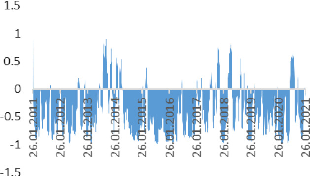
Correlation between Brent Oil prices and RURUSD rate (2011–2021). Source Author calculation, Thomson Reuters
The tendency of significant correlation remained until the middle of 2020, and later the trend for Russia began changing, as the spillover effect between the studied variables became weaker.
In the same period the correlation between Brent oil prices and national currency rates of Algeria is flexible. It does not illustrate any significant pattern of a spillover effect between national currency exchange rates in Algeria (Fig. 11).
Fig. 11.
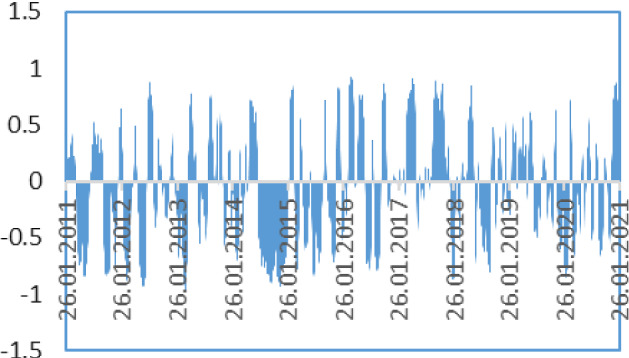
Correlation between Brent Oil prices and DZDUSD rate (2011–2021). Source Author calculation, Thomson Reuters
Also, in the same period the correlation between Brent oil prices and national currencies rates of Nigeria is flexible as well. It does not illustrate any significant pattern of a spillover effect between national currency exchange rates in Nigeria (Fig. 12).
Fig. 12.
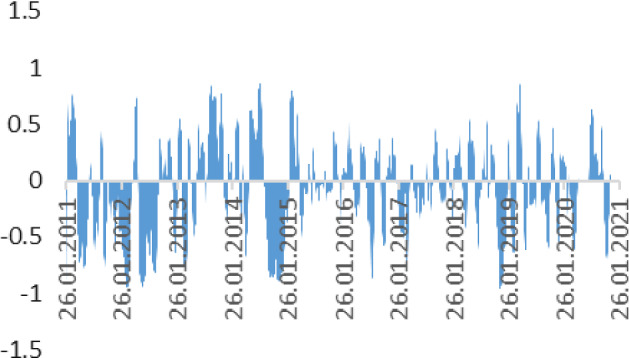
Correlation between Brent Oil prices and NGNUSD rate (2011–2021). Source Author calculation, Thomson Reuters
For the last year correlation parameters became weaker, as the coefficient fluctuates between − 0.5 and 0.5. However, the spillover effect is more significant (in the range from − 0.8 to − 0.1) before 2020. Nigerian Naira and Algerian Dinar were showing nearly the same movements, while the Russian Ruble was in a different corridor. It could have been caused by factors of anti-Russian sanction speeches.
Analysis of Risk-Based Oil Market Spillovers in the Global Crisis Periods with integrated Decision Recommendation System
In the fuzzy decision-making analysis, the first phase is related to imputing the missing expert decisions for the risk-based oil market performance and global crisis periods. The risk-based oil market performance and global crisis periods are defined in Tables 4 and 5.
Table 4.
Determinants of risk-based oil market performance
| Determinants |
|---|
| Currency rates (D1) |
| Oil prices (D2) |
| Systematic risks (D3) |
| Systemic risks (D4) |
Table 5.
Selected global crisis periods
| Periods |
|---|
| Energy crisis (2003–2009) (P1) |
| Global economic recession (2007–2009) (P2) |
| COVID (2019-present) (P3) |
Preference ratings of the experts are collected for the relation and decision matrices. For this purpose, the degrees and scales in Table 6 are used.
Table 6.
Scales and degrees
| Scales | Positive Degrees | Negative Degrees | ||||
|---|---|---|---|---|---|---|
| Determinants | Periods | Preference numbers | MED | NED | MED | NED |
| No (n) | Weakest (w) | 1 | 0.40 | 0.25 | − 0.60 | − 0.37 |
| Some (s) | Poor (p) | 2 | 0.45 | 0.28 | − 0.55 | − 0.34 |
| Medium (m) | Fair (f) | 3 | 0.50 | 0.31 | − 0.50 | − 0.31 |
| High (h) | Good (g) | 4 | 0.55 | 0.34 | − 0.45 | − 0.28 |
| Very high (vh) | Best (b) | 5 | 0.60 | 0.37 | − 0.40 | − 0.25 |
Table 6 shows that No (n), some (s), medium (m), high (h), very high (vh) of determinants of risk-based oil market performance connected with different picture fuzzy numbers. Table 7 includes preference ratings.
Table 7.
The preference ratings of the experts for the relation matrix of determinants
| Expert 1 | Expert 2 | Expert 3 | Expert 4 | Expert 5 | Expert 6 | |
|---|---|---|---|---|---|---|
| D1–D2 | 3 | n/a | 5 | 3 | n/a | 4 |
| D1–D3 | 5 | 5 | 2 | n/a | 5 | n/a |
| D1–D4 | 2 | 2 | n/a | 4 | 4 | 3 |
| D2–D1 | 3 | 2 | 2 | n/a | 3 | n/a |
| D2–D3 | n/a | n/a | 4 | 5 | 3 | n/a |
| D2–D4 | 4 | 4 | n/a | n/a | 3 | n/a |
| D3–D1 | n/a | 5 | 5 | 4 | n/a | 5 |
| D3–D2 | 2 | 3 | n/a | 1 | n/a | 5 |
| D3–D4 | 4 | n/a | 2 | 2 | 3 | n/a |
| D4–D1 | 4 | 2 | 3 | n/a | n/a | 2 |
| D4–D2 | n/a | 1 | 1 | 2 | 5 | n/a |
| D4–D3 | 5 | 3 | n/a | 2 | 5 | n/a |
Table 7 shows the preference ratings of the experts for the relation matrix of determinants of risk-based oil market performance connected with different picture fuzzy numbers. Preference ratings regarding decision matrix are given in Table 8.
Table 8.
The preference ratings of the experts for the decision matrix
| Expert 1 | Expert 2 | Expert 3 | Expert 4 | Expert 5 | Expert 6 | |
|---|---|---|---|---|---|---|
| D1–P1 | n/a | 5 | n/a | 3 | 4 | n/a |
| D1–P2 | 4 | 5 | 3 | n/a | n/a | 5 |
| D1–P3 | 2 | n/a | 4 | 5 | n/a | 4 |
| D2–P1 | n/a | 3 | n/a | 5 | n/a | n/a |
| D2–P2 | 5 | 2 | n/a | 3 | 5 | 2 |
| D2–P3 | 2 | 3 | 4 | n/a | 3 | n/a |
| D3–P1 | 1 | n/a | 5 | 5 | 3 | 2 |
| D3–P2 | 3 | 4 | 2 | n/a | n/a | 3 |
| D3–P3 | 2 | n/a | 1 | 4 | n/a | 2 |
| D4–P1 | 4 | 4 | n/a | 3 | 5 | n/a |
| D4–P2 | n/a | 4 | 3 | n/a | 3 | 4 |
| D4–P3 | n/a | 4 | 4 | n/a | 2 | 3 |
The missing evaluations are completed utilizing the collaborative filtering methodology. In the next step, the similarity degrees of the experts for the relation and decision matrices are calculated in Table 9.
Table 9.
Similarity index matrix of the experts for the determinants
| Expert 1 | Expert 2 | Expert 3 | Expert 4 | Expert 5 | Expert 6 | |
|---|---|---|---|---|---|---|
| Expert 1 | 1.00 | 0.39 | − 0.19 | − 0.05 | 0.33 | − 0.18 |
| Expert 2 | 0.39 | 1.00 | 0.44 | 0.20 | − 0.01 | 0.48 |
| Expert 3 | − 0.19 | 0.44 | 1.00 | 0.51 | − 0.24 | 0.27 |
| Expert 4 | − 0.05 | 0.20 | 0.51 | 1.00 | − 0.31 | − 0.19 |
| Expert 5 | 0.33 | − 0.01 | − 0.24 | − 0.31 | 1.00 | − 0.01 |
| Expert 6 | − 0.18 | 0.48 | 0.27 | − 0.19 | − 0.01 | 1.00 |
Table 9 shows similarity index matrix of the experts for the determinants. The preference ratings of the experts for the relation matrix of determinants. Table 10 includes similarity index matrix.
Table 10.
Similarity index matrix of the experts for the periods
| Expert 1 | Expert 2 | Expert 3 | Expert 4 | Expert 5 | Expert 6 | |
|---|---|---|---|---|---|---|
| Expert 1 | 1.00 | − 0.15 | − 0.25 | − 0.68 | 0.62 | 0.19 |
| Expert 2 | − 0.15 | 1.00 | − 0.11 | − 0.07 | − 0.23 | 0.54 |
| Expert 3 | − 0.25 | − 0.11 | 1.00 | 0.30 | − 0.26 | 0.06 |
| Expert 4 | − 0.68 | − 0.07 | 0.30 | 1.00 | − 0.57 | 0.12 |
| Expert 5 | 0.62 | − 0.23 | − 0.26 | − 0.57 | 1.00 | − 0.15 |
| Expert 6 | 0.19 | 0.54 | 0.06 | 0.12 | − 0.15 | 1.00 |
The next step is related to the prediction of the missing expert evaluations with the normalized similarity values iteratively. Completed evaluations are shown in Tables 11 and 12.
Table 11.
Completed expert evaluations for the determinants
| Expert 1 | Expert 2 | Expert 3 | Expert 4 | Expert 5 | Expert 6 | |
|---|---|---|---|---|---|---|
| D1–D2 | 3 | 4 (Iteration 1) | 5 | 3 | 3 (Iteration 1) | 4 |
| D1–D3 | 5 | 5 | 2 | 2 (Iteration 1) | 5 | 5 (Iteration 1) |
| D1–D4 | 2 | 2 | 4 (Iteration 1) | 4 | 4 | 3 |
| D2–D1 | 3 | 2 | 2 | 2 (Iteration 1) | 3 | 2 (Iteration 1) |
| D2–D3 | 3 (Iteration 2) | 4 (Iteration 2) | 4 | 5 | 3 | 4 (Iteration 2) |
| D2–D4 | 4 | 4 | 4 (Iteration 2) | 4 (Iteration 2) | 3 | 4 (Iteration 1) |
| D3–D1 | 5 (Iteration 1) | 5 | 5 | 4 | 5 (Iteration 2) | 5 |
| D3–D2 | 2 | 3 | 1 (Iteration 1) | 1 | 2 (Iteration 1) | 5 |
| D3–D4 | 4 | 2 (Iteration 2) | 2 | 2 | 3 | 2 (Iteration 2) |
| D4–D1 | 4 | 2 | 3 | 3 (Iteration 1) | 4 (Iteration 1) | 2 |
| D4–D2 | 1 (Iteration 1) | 1 | 1 | 2 | 5 | 1 (Iteration 1) |
| D4–D3 | 5 | 3 | 2 (Iteration 1) | 2 | 5 | 3 (Iteration 1) |
Table 12.
Completed expert evaluations for the periods
| Expert 1 | Expert 2 | Expert 3 | Expert 4 | Expert 5 | Expert 6 | |
|---|---|---|---|---|---|---|
| D1–P1 | 4 (Iteration 1) | 5 | 3 (Iteration 1) | 3 | 4 | 5 (Iteration 1) |
| D1–P2 | 4 | 5 | 3 | 3 (Iteration 1) | 4 (Iteration 1) | 5 |
| D1–P3 | 2 | 4 (Iteration 1) | 4 | 5 | 2 (Iteration 1) | 4 |
| D2–P1 | 3 (Iteration 3) | 3 | 5 (Iteration 1) | 5 | 3 (Iteration 3) | 3 (Iteration 1) |
| D2–P2 | 5 | 2 | 3 (Iteration 1) | 3 | 5 | 2 |
| D2–P3 | 2 | 3 | 4 | 4 (Iteration 1) | 3 | 3 (Iteration 1) |
| D3–P1 | 1 | 2 (Iteration 1) | 5 | 5 | 3 | 2 |
| D3–P2 | 3 | 4 | 2 | 2 (Iteration 1) | 3 (Iteration 1) | 3 |
| D3–P3 | 2 | 2 (Iteration 1) | 1 | 4 | 2 (Iteration 1) | 2 |
| D4–P1 | 4 | 4 | 3 (Iteration 1) | 3 | 5 | 4 (Iteration 1) |
| D4–P2 | 3 (Iteration 1) | 4 | 3 | 3 (Iteration 1) | 3 | 4 |
| D4–P3 | 2 (Iteration 1) | 4 | 4 | 4 (Iteration 1) | 2 | 3 |
Table 11 shows completed expert evaluations for the determinants.
Table 12 shows completed expert evaluations for the periods. The second phase of the proposed model includes weighting the determinants of risk-based oil market performance. Linguistic evaluations of experts for the determinants are defined in Table 13.
Table 13.
Linguistic evaluations of experts for the determinants
| D1 | D2 | D3 | D4 | D1 | D2 | D3 | D4 | |
|---|---|---|---|---|---|---|---|---|
| Expert 1 | Expert 2 | |||||||
| D1 | M | VH | S | H | VH | S | ||
| D2 | M | M | H | S | H | H | ||
| D3 | VH | S | H | VH | M | S | ||
| D4 | H | N | VH | S | N | M | ||
| Expert 3 | Expert 4 | |||||||
| D1 | VH | S | H | M | S | H | ||
| D2 | S | H | H | S | VH | H | ||
| D3 | VH | N | S | H | N | S | ||
| D4 | M | N | S | M | S | S | ||
| Expert 5 | Expert 6 | |||||||
| D1 | M | VH | H | H | VH | M | ||
| D2 | M | M | M | S | H | H | ||
| D3 | VH | S | M | VH | VH | S | ||
| D4 | H | VH | VH | S | N | M | ||
Table 13 shows linguistic evaluations of experts for the determinants. Next, average values of positive and negative membership and non-membership degrees are defined for the determinants as in Table 14.
Table 14.
Average values of positive and negative membership and non-membership degrees for the determinants
| D1 | D2 | D3 | D4 | |||||||||||||
|---|---|---|---|---|---|---|---|---|---|---|---|---|---|---|---|---|
| Positive degrees | Negative degrees | Positive degrees | Negative degrees | Positive degrees | Negative degrees | Positive degrees | Negative degrees | |||||||||
| μ | n | μ | n | μ | n | μ | n | μ | n | μ | n | μ | N | μ | n | |
| D1 | – | – | – | – | 0.53 | 0.33 | − 0.47 | − 0.29 | 0.55 | 0.34 | − 0.45 | − 0.28 | 0.51 | 0.31 | − 0.49 | − 0.30 |
| D2 | 0.47 | 0.29 | − 0.53 | − 0.33 | – | – | – | – | 0.54 | 0.33 | − 0.46 | − 0.28 | 0.54 | 0.33 | − 0.46 | − 0.28 |
| D3 | 0.59 | 0.37 | − 0.41 | − 0.25 | 0.47 | 0.29 | − 0.53 | − 0.33 | – | – | – | – | 0.48 | 0.29 | − 0.53 | − 0.32 |
| D4 | 0.50 | 0.31 | − 0.50 | − 0.31 | 0.44 | 0.27 | − 0.56 | − 0.35 | 0.52 | 0.32 | − 0.48 | − 0.30 | – | – | – | – |
Table 14 shows average values of positive and negative membership and non-membership degrees for the determinants. Score functions are shown in Table 15.
Table 15.
Score function values of the determinants for bipolar q-ROFSs
| D1 | D2 | D3 | D4 | |
|---|---|---|---|---|
| D1 | 0.000 | 0.194 | 0.197 | 0.191 |
| D2 | 0.194 | 0.000 | 0.195 | 0.195 |
| D3 | 0.210 | 0.194 | 0.000 | 0.192 |
| D4 | 0.191 | 0.199 | 0.192 | 0.000 |
The sj, kj, qj, and wj values are computed for the relationship degrees of each determinant in Table 16.
Table 16.
Sj, kj, qj, and wj values for the relationship degrees of each determinant
| D1 | Sj | Kj | qj | wj | D2 | Sj | kj | Qj | Wj |
|---|---|---|---|---|---|---|---|---|---|
| D3 | 0.197 | 1.000 | 1.000 | 0.394 | D4 | 0.195 | 1.000 | 1.000 | 0.352 |
| D2 | 0.194 | 1.194 | 0.838 | 0.330 | D3 | 0.195 | 1.000 | 1.000 | 0.352 |
| D4 | 0.191 | 1.191 | 0.703 | 0.277 | D1 | 0.194 | 1.194 | 0.838 | 0.295 |
| D3 | Sj | kj | qj | wj | D4 | Sj | kj | Qj | Wj |
|---|---|---|---|---|---|---|---|---|---|
| D1 | 0.210 | 1.000 | 1.000 | 0.394 | D2 | 0.199 | 1.000 | 1.000 | 0.393 |
| D2 | 0.194 | 1.194 | 0.838 | 0.330 | D3 | 0.192 | 1.192 | 0.839 | 0.330 |
| D4 | 0.192 | 1.192 | 0.703 | 0.277 | D1 | 0.191 | 1.191 | 0.705 | 0.277 |
Relation matrix is created in Table 17.
Table 17.
Relation Matrix with the values of wj
| D1 | D2 | D3 | D4 | |
|---|---|---|---|---|
| D1 | 0.330 | 0.394 | 0.277 | |
| D2 | 0.295 | 0.352 | 0.352 | |
| D3 | 0.394 | 0.330 | 0.277 | |
| D4 | 0.277 | 0.393 | 0.330 |
Table 18 explains the stable matrix.
Table 18.
Stable matrix
| D1 | D2 | D3 | D4 | |
|---|---|---|---|---|
| D1 | 0.245 | 0.245 | 0.245 | 0.245 |
| D2 | 0.259 | 0.259 | 0.259 | 0.259 |
| D3 | 0.264 | 0.264 | 0.264 | 0.264 |
| D4 | 0.232 | 0.232 | 0.232 | 0.232 |
Figure 13 includes causal diagrams of the determinants.
Fig. 13.
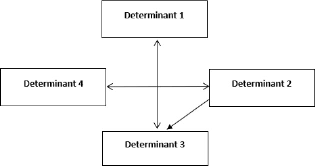
Impact-relation map for the determinants
Systematic risks are affected by currency rates and oil prices. Furthermore, oil prices and systemic risks have an influence on each other. The weights of the items are given in Table 19.
Table 19.
Comparative weighting priorities for the determinants
| Bipolar IFSs | Bipolar PFSs | Bipolar q-ROFSs | |
|---|---|---|---|
| D1 | 3 | 3 | 3 |
| D2 | 2 | 2 | 2 |
| D3 | 1 | 1 | 1 |
| D4 | 4 | 4 | 4 |
Systematic risks have the greatest importance for oil market performance. Moreover, oil prices also play a key role in this situation. The final phase of the proposed model focuses on ranking the global crisis periods with respect to the risk-based oil market determinants. Table 20 shows the evaluations.
Table 20.
Linguistic evaluations of experts for the positive and negative degrees of periods
| D1 | D2 | D3 | D4 | D1 | D2 | D3 | D4 | ||
|---|---|---|---|---|---|---|---|---|---|
| Expert 1 | Expert 2 | ||||||||
| P1 | G | F | W | G | B | F | P | G | |
| P2 | G | B | F | F | B | P | G | G | |
| P3 | P | P | P | P | G | F | P | G | |
| Expert 3 | Expert 4 | ||||||||
| P1 | F | B | B | F | F | B | B | F | |
| P2 | F | F | P | F | F | F | P | F | |
| P3 | G | G | W | G | B | G | G | G | |
| Expert 5 | Expert 6 | ||||||||
| P1 | G | F | F | B | B | F | P | G | |
| P2 | G | B | F | F | B | P | F | G | |
| P3 | P | F | P | P | G | F | P | F | |
Table 21 indicates the average values.
Table 21.
Average values of positive and negative membership and non-membership degrees for the periods
| D1 | D2 | D3 | D4 | |||||||||||||
|---|---|---|---|---|---|---|---|---|---|---|---|---|---|---|---|---|
| Positive Degrees | Negative Degrees | Positive Degrees | Negative Degrees | Positive Degrees | Negative Degrees | Positive Degrees | Negative Degrees | |||||||||
| μ | n | μ | n | μ | n | μ | n | μ | N | μ | n | μ | n | μ | N | |
| P1 | 0.55 | 0.34 | − 0.45 | − 0.28 | 0.53 | 0.33 | − 0.47 | − 0.29 | 0.50 | 0.31 | − 0.50 | − 0.31 | 0.54 | 0.33 | − 0.46 | − 0.28 |
| P2 | 0.55 | 0.34 | − 0.45 | − 0.28 | 0.52 | 0.32 | − 0.48 | − 0.30 | 0.49 | 0.30 | − 0.51 | − 0.31 | 0.52 | 0.32 | − 0.48 | − 0.30 |
| P3 | 0.53 | 0.32 | − 0.48 | − 0.29 | 0.51 | 0.31 | − 0.49 | − 0.30 | 0.46 | 0.28 | − 0.54 | − 0.33 | 0.51 | 0.31 | − 0.49 | − 0.30 |
Table 22 includes the score functions.
Table 22.
Score function values of the periods for bipolar q-ROFSs
| Determinants/Periods | D1 | D2 | D3 | D4 |
|---|---|---|---|---|
| P1 | 0.197 | 0.194 | 0.191 | 0.195 |
| P2 | 0.197 | 0.192 | 0.191 | 0.192 |
| P3 | 0.192 | 0.191 | 0.195 | 0.191 |
Normalized matrix is given in Table 23.
Table 23.
Normalized decision matrix
| Determinants/Periods | D1 | D2 | D3 | D4 |
|---|---|---|---|---|
| P1 | 0.582 | 0.582 | 0.573 | 0.584 |
| P2 | 0.582 | 0.576 | 0.574 | 0.574 |
| P3 | 0.569 | 0.574 | 0.585 | 0.573 |
Table 24 explains the weighted matrix.
Table 24.
Weighted decision matrix
| Determinants/Periods | D1 | D2 | D3 | D4 |
|---|---|---|---|---|
| P1 | 0.142 | 0.151 | 0.151 | 0.136 |
| P2 | 0.142 | 0.149 | 0.152 | 0.133 |
| P3 | 0.139 | 0.149 | 0.155 | 0.133 |
Concordance and discordance interval matrixes are created in Table 25.
Table 25.
Concordance and discordance interval matrices
| Periods | Concordance matrix | Discordance matrix | ||||
|---|---|---|---|---|---|---|
| P1 | P2 | P3 | P1 | P2 | P3 | |
| P1 | 0.000 | 0.736 | 0.736 | 0.000 | 0.054 | 1.000 |
| P2 | 0.509 | 0.000 | 0.736 | 1.000 | 0.000 | 0.974 |
| P3 | 0.264 | 0.264 | 0.000 | 0.986 | 1.000 | 0.000 |
Concordance, discordance, and aggregated index matrixes are constructed in Table 26.
Table 26.
Concordance, discordance and aggregated index matrices
| Periods | Concordance Matrix | Discordance Matrix | Aggregated Matrix | ||||||
|---|---|---|---|---|---|---|---|---|---|
| P1 | P2 | P3 | P1 | P2 | P3 | P1 | P2 | P3 | |
| P1 | 0 | 1 | 1 | 1 | 1 | 0 | 0 | 1 | 0 |
| P2 | 0 | 0 | 1 | 0 | 1 | 0 | 0 | 0 | 0 |
| P3 | 0 | 0 | 0 | 0 | 0 | 1 | 0 | 0 | 0 |
Table 27 focuses on the calculation of the net superior, inferior, and overall values for ranking the periods.
Table 27.
Net superior, inferior, and overall values of the periods with bipolar q-ROFSs
| Periods | Net superior values | Net Inferior values | Overall values |
|---|---|---|---|
| P1 | 0.699 | − 0.931 | 1.630 |
| P2 | 0.245 | 0.920 | − 0.675 |
| P3 | − 0.943 | 0.012 | − 0.955 |
The analysis is also performed by IFSs and PFSs. The results are compared in Table 28.
Table 28.
Comparative overall ranking results of the periods
| Periods | Bipolar q-ROF Multi SWARA-ELECTRE | Bipolar PF Multi SWARA-ELECTRE | Bipolar IF Multi SWARA-ELECTRE |
|---|---|---|---|
| P1 | 1 | 1 | 1 |
| P2 | 2 | 2 | 2 |
| P3 | 3 | 3 | 3 |
The results are the same for all different fuzzy numbers that gives an idea about the validity of the model. It is determined that the energy crisis between 2003 and 2009 is the most important period for the efficiency of the oil market performance.
Discussion
By 2021, the level of globalization of financial markets has reached a new level, due to increased capital mobility. This has affected the impact on the flow of funds from institutional investors in emerging markets to global investment portfolios. This figure increased from 1% of the global market capitalization in 1987 to 15% by 2017. And capital market integration is also associated with an enhanced spillover effect between markets (Antonakakis et al., 2013; Baruník & Krehlík, 2018; Basher & Sadorsky, 2016; Basta & Molnar, 2018; Bouri et al., 2017; Broadstock & Filis, 2014).
The results support that strong shocks in oil markets are more quickly transmitted to the exchange rates of oil-producing countries. This article confirms the thesis that the volatility and profitability of assets constantly change synchronously over time. Volatility shocks can lead to shifts in investor behavior and create side effects in the short term. Therefore, investors seeking to improve their risk-adjusted portfolio returns typically adjust their asset allocation to account for the impact of such shocks to reduce contagion risks (Caporale et al., 2015; Chen et al., 2014; Chkili et al., 2014; Diaz et al., 2016; Ding & Liu, 2019; Ding et al., 2017; Du & He, 2015; Dutta, 2017).
This paper proves the idea that the link between the economies of oil-producing countries and the world economy through trade and information flows has increased due to their role as global recipients of investment and major trading partners of the United States (Shahzad et al., 2018; Tursoy & Faisal, 2018).
The empirical findings of recent research have the same direction: in Russia and other oil-producing countries, the development of financial institutions is slow. Therefore, vulnerability to external shocks from developed markets is increasing (Norouzi et al., 2020; Ramelli & Wagner, 2020; Salisu & Akanni, 2020; Szczygielski et al., 2021; Wen et al., 2021; Mazur et al., 2021; Narayan, 2020; Nguyen et al., 2021; Fang et al., 2021; Szczygielski et al., 2021; Wen et al., 2021).
This model allows to measure the correlation coefficient to identify the joint movement of a group of markets. You can also determine the strength of the relationship between the profitability of the currencies of oil-producing countries and oil prices. The impact of volatility is considered both in the pre-crisis and post-crisis periods using daily price fluctuations. All three recent shocks (2008, 2012, 2020) in the oil market are transmitted to the currency markets of oil-producing countries. At the same time, the latest shock of 2020 caused by the COVID-19 pandemic has not yet been fully transmitted to the Russian ruble exchange rate. The main reason for this is the factor of reducing the sanctions pressure and the low level of external public debt in Russia.
Many researchers have identified a strong increase in the correlations between oil prices and the yield of the currencies of oil-producing countries over the past two decades. The points of shocks to the volatility of national currencies coincide with sharp fluctuations in oil prices. This confirms the findings, which also revealed a large financial dependence on the United States for Brazil and the Russian national currency during the global economic crisis (Vo, 2011; Wen et al., 2019; Whaley, 2000).
Despite the growing global focus on oil prices, relevant empirical research on spillovers remains surprisingly limited, confirming the need for further analysis. For example, correlations between national currencies of oil-producing countries are usually estimated using a variance–covariance matrix, which cannot estimate the direction and intensity of side effects over time. Understanding the direction of spillovers is important for developing optimal portfolio and risk management strategies, including hedging practices, and providing policy makers with information about potential cross-country sources of business fluctuations (Ahmad et al., 2018).
Many studies have extensively used the financial markets and asset classes spillover index method to measure the magnitude and direction of spillover effects (Maghyereh et al., 2016; Nadal et al., 2017; Sarwar et al., 2019).
This article fills in the gap in the body of knowledge, as its results better reflect the dynamic interactions between oil prices and currencies. For example, daily stock data causes non-synchronous trading day offsets and the impact of liquidity on the stock price, while monthly data cannot identify the transmission of volatility due to time aggregation offsets and offsetting effects.
Thus, the financial crises have increased the contagion effect between the oil market and the currency markets of oil-producing countries. Other studies show similar results in stock markets, as well as between commodity and currency markets.
For the pre-crisis period, it was assumed that financial uncertainty has a negative impact on both returns and the side effects of volatility, indicating that risk aversion by investors may have reduced the side effects in stock markets during this period. However, the dynamics of oil price volatility shows that along with the Brazilian stock market, the Russian stock market has recently begun to play an important role as a source of information transmission. The result confirms the payback hypothesis (contagion effect), which assumes a decrease in the benefits of portfolio diversification in commodity markets during crisis periods. This finding is consistent with findings where a mixed portfolio of commodity assets provides reduced benefits through both improved diversification and reduced risk over these periods (Dutta et al., 2017; Foroni et al., 2017; Haugom et al., 2014).
The oil market is always a transmitter of volatility, and the national currency markets of oil-producing countries become net consumers of investment in the post-crisis period. When predicting the exposure to portfolio market risks and determining whether the diversification benefits are available in the oil market, it is necessary to take into account the impact of side effects on the reduction of the diversification benefits, especially during periods of turmoil. In terms of asset allocation, the intensity of the side effects creates the need (or opportunity) to build a new diversification strategy. For example, portfolio investors in the markets can direct their funds to the oil market, which potentially reduces the risk of price declines in an environment of increased secondary investment intensity during periods of turmoil (Ji & Fan, 2016; Jin et al., 2020; Joo & Park, 2017).
Finally, in light of the interest in the impact of oil market volatility on macroeconomic indicators, identifying the presence, significance and changes in the net effects of volatility between the oil market and the currency markets of oil-producing countries offers directions for future research, which includes analyzing the impact of volatility in financial markets on real economic activity, understanding the significance of this volatility as sources of structural changes in the currency markets of oil-producing countries.
Systematic risks are the most important risk type for the performance of oil markets. Systematic risk sources can be defined as market risk, political risk, inflation risk, interest rate risk and currency risk. These issues indicate the issues that investors cannot intervene on their own. Therefore, to increase the performance of oil markets, it is vital for countries to achieve economic stability first. In this context, country governments must first solve the high inflation problem and reduce the uncertainty in the market. In parallel, there should be no political risk in the country. In addition, factors that are important to the country's economy, such as interest rate and exchange rate, should not increase radically or decrease. In this way, it will be possible for countries to reach more efficient oil markets.
Conclusions
Current trends in the structure of the currency market of oil-producing countries are created by the flow of volatility between national stock indices and the oil market. After the beginning of the pandemic crisis in 2020, the expectations of market participants began to correspond more to the hypothesis of rationality, in particular, the horizon of inflation expectations expanded, and the predictability of maintaining low interest rates in the world increased. In addition, the long-term trends include low inflation and a stimulating monetary policy.
The article reveals that the latest shock of 2020, caused by the covid-19 pandemic, has not yet been fully transmitted to the Russian ruble exchange rate. The main reason for this is the factor of reducing sanctions pressure and the low level of external public debt in Russia. For the last year correlation parameters became weaker, as the RURUSD correlation coefficient is fluctuating between − 0.5 and 0.5. However, before 2020 the spillover effect is more significant (in the range from − 0.8 to − 0.1). Nigerian Naira and Algerian Dinar were showing almost the same movements, while Russian Ruble was in different corridor.
The managerial implications of the empirical results are including: the results can be useful in the formation of forecasts of asset prices and asset volatility by central banks. Some aspects outlined in the dissertation research can also be used in the activities of analytical departments of banks, investment funds and consulting companies. It can be integrated into the educational process of financial and economic universities.
The area for future research is in evaluating spillover effects on currency exchange rates in all oil exporting countries. Additionally, another evaluation is also performed regarding risk-based oil market spillovers in the global crisis periods with integrated decision recommendation systems. For this purpose, a fuzzy decision-making model is created by considering bipolar q-ROFSs, M-SWARA, ELECTRE and imputation of expert evaluations with collaborative filtering. It is defined that systematic risks are affected by currency rates and oil prices.
The major limitation is that: oil prices and systemic risks have an influence on each other. The findings also state that systematic risks have the greatest importance for oil market performance. Moreover, oil prices also play a key role in this situation. With respect to the ranking results of the periods, it is determined that the energy crisis between 2003 and 2009 is the most important period for the efficiency of the oil market performance.
Authors’ contributions
The problem is proposed by IMB. The solving method is proposed by HD and SY. The method is applied by HD and SY. The writing of manuscript is done by AM. All authors read and approved the final manuscript.
Funding
This research received no external funding.
Availability of data and materials
In this study the data is not available.
Declarations
Ethics approval and consent to participate
This manuscript does not require ethical approval and content to participate since it does not contain any human participate, human data or human tissue.
Competing interests
There was no conflict or competing interest for the authors in establishing this manuscript. This manuscript has not been published or presented elsewhere in part or in entirety and is not under consideration by another journal. We have read and understood your journal’s policies, and we believe that neither the manuscript nor the study violates any of these. There are no conflicts of interest to declare.
Footnotes
Publisher's Note
Springer Nature remains neutral with regard to jurisdictional claims in published maps and institutional affiliations.
Contributor Information
Alexey Mikhaylov, Email: ayumihajlov@fa.ru.
Ishaq M. Bhatti, Email: i.bhatti@latrobe.edu.au
Hasan Dinçer, Email: hdincer@medipol.edu.tr.
Serhat Yüksel, Email: serhatyuksel@medipol.edu.tr.
References
- Ahmad W, Sadorsky P, Sharma A. Optimal hedge ratios for clean energy equities. Economic Modelling. 2018;72:278–295. doi: 10.1016/j.econmod.2018.02.008. [DOI] [Google Scholar]
- Al-Awadhi AM, Alsaifi K, Al-Awadhi A, et al. Death and contagious infectious diseases: Impact of the COVID-19 virus on stock market returns. Journal of Behavioral and Experimental Finance. 2020;27:100326. doi: 10.1016/j.jbef.2020.100326. [DOI] [PMC free article] [PubMed] [Google Scholar]
- Aliyu SUR. Exchange rate volatility and export trade in Nigeria: An empirical investigation. Applied Financial Economics. 2010;20(13):1071–1084. doi: 10.1080/09603101003724380. [DOI] [Google Scholar]
- Altig D, Baker S, Barrero JM, et al. Economic uncertainty before and during the COVID-19 pandemic. Journal of Public Economics. 2020;191:104274. doi: 10.1016/j.jpubeco.2020.104274. [DOI] [PMC free article] [PubMed] [Google Scholar]
- Antonakakis N, Chatziantoniou I, Filis G. Dynamic co-movements of stock market returns, implied volatility and policy uncertainty. Economics Letters. 2013;120(1):87–92. doi: 10.1016/j.econlet.2013.04.004. [DOI] [Google Scholar]
- Atanassov, K. T. (1999). Intuitionistic fuzzy sets. In Intuitionistic fuzzy sets (pp. 1–137). Physica, Heidelberg.
- Bahmani-Oskooee M, Aftab M. On the asymmetric effects of exchange rate volatility on trade flows: New evidence from us-malaysia trade at the industry level. Economic Modelling. 2017;63:86–103. doi: 10.1016/j.econmod.2017.02.004. [DOI] [Google Scholar]
- Bahmani-Oskooee M, Wang Y. United states-china trade at the commodity level and the yuan-dollar exchange rate. Contemporary Economic Policy. 2007;25(3):341–361. doi: 10.1111/j.1465-7287.2007.00049.x. [DOI] [Google Scholar]
- Baruník J, Krehlík T. Measuring the frequency dynamics of financial connectedness and systemic risk. Journal of Financial Economics. 2018;16(2):271–296. doi: 10.1093/jjfinec/nby001. [DOI] [Google Scholar]
- Basher SA, Sadorsky P. Hedging emerging market stock prices with oil, gold, VIX, and bonds: A comparison between DCC, ADCC and GO-GARCH. Energy Economics. 2016;54:235–247. doi: 10.1016/j.eneco.2015.11.022. [DOI] [Google Scholar]
- Basta M, Molnar P. Oil market volatility and stock market volatility. Finance Research Letters. 2018;26:204–214. doi: 10.1016/j.frl.2018.02.001. [DOI] [Google Scholar]
- Belluscio V, Iosa M, Vannozzi G, Paravati S, Peppe A. Auditory Cue based on the Golden ratio can improve gait patterns in people with Parkinson’s disease. Sensors. 2021;21(3):911. doi: 10.3390/s21030911. [DOI] [PMC free article] [PubMed] [Google Scholar]
- Benayoun R, Roy B, Sussman B. ELECTRE: Une méthode pour guider le choix en présence de points de vue multiples. Note De Travail. 1966;49:2–120. [Google Scholar]
- Bhuiyan MA, Dinçer H, Yüksel S, Mikhaylov A, Danish MSS, Pinter G, Uyeh DD, Stepanova D. Economic indicators and bioenergy supply in developed economies: QROF-DEMATEL and random forest models. Energy Reports. 2022;8(2022):561–570. doi: 10.1016/j.egyr.2021.11.278. [DOI] [Google Scholar]
- Bouri E, Jain A, Biswal PC, Roubaud D. Cointegration and nonlinear causality amongst gold, oil, and the Indian stock market: Evidence from implied volatility indices. Resources Policy. 2017;52:201–206. doi: 10.1016/j.resourpol.2017.03.003. [DOI] [Google Scholar]
- Broadstock DC, Filis G. Oil price shocks and stock market returns: New evidence from the United States and China. Journal of International Financial Markets, Institutions and Money. 2014;33:417–433. doi: 10.1016/j.intfin.2014.09.007. [DOI] [Google Scholar]
- Caporale GM, Menla Ali F, Spagnolo N. Oil price uncertainty and sectoral stock returns in China: A time-varying approach. China Economic Review. 2015;34:311–321. doi: 10.1016/j.chieco.2014.09.008. [DOI] [Google Scholar]
- Chen W, Hamori S, Kinkyo T. Macroeconomic impacts of oil prices and underlying financial shocks. Journal of International Financial Markets, Institutions and Money. 2014;29:1–12. doi: 10.1016/j.intfin.2013.11.006. [DOI] [Google Scholar]
- Chkili W, Aloui C, Nguyen DK. Instabilities in the relationships and hedging strategies between crude oil and US stock markets: Do long memory and asymmetry matter? Journal of International Financial Markets, Institutions and Money. 2014;33:354–366. doi: 10.1016/j.intfin.2014.09.003. [DOI] [Google Scholar]
- Diaz EM, Molero JC, Perez de Gracia F. Oil price volatility and stock returns in the G7 economies. Energy Economics. 2016;54:417–430. doi: 10.1016/j.eneco.2016.01.002. [DOI] [Google Scholar]
- Ding Z, Liu Z. Research on the Mechanism of Coal Price Fluctuation and Its Impact on Chinese Economy. China University of Mining and Technology Press; 2019. [Google Scholar]
- Ding Z, Liu Z, Zhang Y, Long R. The contagion effect of international crude oil price fluctuations on Chinese stock market investor sentiment. Applied Energy. 2017;187:27–36. doi: 10.1016/j.apenergy.2016.11.037. [DOI] [Google Scholar]
- Du L, He Y. Extreme risk spillovers between crude oil and stock markets. Energy Economics. 2015;51:455–465. doi: 10.1016/j.eneco.2015.08.007. [DOI] [Google Scholar]
- Dutta A. Oil price uncertainty and clean energy stock returns: New evidence from crude oil volatility index. Journal of Cleaner Production. 2017;164:1157–1166. doi: 10.1016/j.jclepro.2017.07.050. [DOI] [Google Scholar]
- Dutta A. Oil and energy sector stock markets: An analysis of implied volatility indexes. Journal of Multinational Financial Management. 2018;44:61–68. doi: 10.1016/j.mulfin.2017.12.002. [DOI] [Google Scholar]
- Dutta A, Nikkinen J, Rothovius T. Impact of oil price uncertainty on Middle East and African stock markets. Energy. 2017;123:189–197. doi: 10.1016/j.energy.2017.01.126. [DOI] [Google Scholar]
- Fang Y, Jing J, Shi Y, Zhao Y. Financial spillovers and spillbacks: New evidence from China and G7 countries. Economic Modelling. 2021;94:184–200. doi: 10.1016/j.econmod.2020.09.022. [DOI] [Google Scholar]
- Foroni C, Guerin P, Marcellino M. Explaining the time-varying effects of oil market shocks on US stock returns. Economic Letters. 2017;155:84–88. doi: 10.1016/j.econlet.2017.03.017. [DOI] [Google Scholar]
- Haugom E, Langeland H, Molnar P, Westgaard S. Forecasting volatility of the US oil market. Journal of Banking & Finance. 2014;47:1–14. doi: 10.1016/j.jbankfin.2014.05.026. [DOI] [Google Scholar]
- Jammazi R, Ferrer R, Jareno F, Shahzad SJH. Time-varying causality between crude oil and stock markets: What can we learn from a multiscale perspective? International Review of Economics & Finance. 2017;49:453–483. doi: 10.1016/j.iref.2017.03.007. [DOI] [Google Scholar]
- Ji Q, Bouri E, Roubaud D. Dynamic network of implied volatility transmission among US equities, strategic commodities, and BRICS equities. International Review of Financial Analysis. 2018;57:1–12. doi: 10.1016/j.irfa.2018.02.001. [DOI] [Google Scholar]
- Ji Q, Fan Y. Modelling the joint dynamics of oil prices and investor fear gauge. Research in International Business and Finance. 2016;37:242–251. doi: 10.1016/j.ribaf.2015.11.016. [DOI] [Google Scholar]
- Jin J, Han L, Wu L, Zeng H. The hedging effectiveness of global sectors in emerging and developed stock markets. International Review of Economics & Finance. 2020;66:92–117. doi: 10.1016/j.iref.2019.11.001. [DOI] [Google Scholar]
- Joo YC, Park SY. Oil prices and stock markets: Does the effect of uncertainty change over time? Energy Economics. 2017;61:42–51. doi: 10.1016/j.eneco.2016.10.017. [DOI] [Google Scholar]
- Keršuliene V, Zavadskas EK, Turskis Z. Selection of rational dispute resolution method by applying new step-wise weight assessment ratio analysis (SWARA) Journal of Business Economics and Management. 2010;11(2):243–258. doi: 10.3846/jbem.2010.12. [DOI] [Google Scholar]
- Liu F, Lee HJ. Use of social network information to enhance collaborative filtering performance. Expert Systems with Applications. 2010;37(7):4772–4778. doi: 10.1016/j.eswa.2009.12.061. [DOI] [Google Scholar]
- Maghyereh AI, Awartani B, Bouri E. The directional volatility connectedness between crude oil and equity markets: New evidence from implied volatility indexes. Energy Economics. 2016;57:78–93. doi: 10.1016/j.eneco.2016.04.010. [DOI] [Google Scholar]
- Mazur M, Dang M, Vega M. COVID-19 and the March 2020 stock market crash. Evidence from S&P 1500. Finance Research Letters. 2021;38:101690. doi: 10.1016/j.frl.2020.101690. [DOI] [PMC free article] [PubMed] [Google Scholar]
- Mikhaylov A. Volatility spillover effect between stock and exchange rate in oil exporting countries. International Journal of Energy Economics and Policy. 2018;8(3):321–326. [Google Scholar]
- Nadal R, Szklo A, Lucena A. Time-varying impacts of demand and supply oil shocks on correlations between crude oil prices and stock markets indices. Research in International Business and Finance. 2017;42:1011–1020. doi: 10.1016/j.ribaf.2017.07.037. [DOI] [Google Scholar]
- Narayan PK. Oil price news and COVID-19—is there any connection? [J] Energy Research Letters. 2020;1(1):13176. doi: 10.46557/001c.13176. [DOI] [Google Scholar]
- Nguyen, X. P., Hoang, A. T., ¨Olçer, A. I., & Huynh T. T. (2021). Record decline in global CO2 emissions prompted by COVID-19 pandemic and its implications on future climate change policies. Energy Sources, Part A: Recovery, Utilization, and Environmental, 1–4.
- Norouzi N, de Rubens GZ, Choupanpiesheh S, et al. When pandemics impact economies and climate change: Exploring the impacts of COVID-19 on oil and electricity demand in China. Energy Research & Social Science. 2020;68:101654. doi: 10.1016/j.erss.2020.101654. [DOI] [PMC free article] [PubMed] [Google Scholar]
- Ramelli S, Wagner AF. Feverish stock price reactions to COVID-19. The Review of Corporate Finance Studies. 2020;9(3):622–655. doi: 10.1093/rcfs/cfaa012. [DOI] [Google Scholar]
- Salisu AA, Akanni LO. Constructing a global fear index for the COVID-19 pandemic. Emerging Markets Finance & Trade. 2020;56(10):2310–2331. doi: 10.1080/1540496X.2020.1785424. [DOI] [Google Scholar]
- Sarwar S, Khalfaoui R, Waheed R, Dastgerdi HG. Volatility spillovers and hedging: Evidence from Asian oil-importing countries. Resources Policy. 2019;61:479–488. doi: 10.1016/j.resourpol.2018.04.010. [DOI] [Google Scholar]
- Shahzad SJH, Mensi W, Hammoudeh S, Rehman MU, Al-Yahyaee KH. Extreme dependence and risk spillovers between oil and Islamic stock markets. Emerging Markets Review. 2018;34:42–63. doi: 10.1016/j.ememar.2017.10.003. [DOI] [Google Scholar]
- Szczygielski, J. J., Bwanya, P. R., Charteris, A., & Brzeszczyński, J. (2021). The only certainty is uncertainty: An analysis of the impact of COVID-19 uncertainty on regional stock markets. Finance Research Letters, 101945. [DOI] [PMC free article] [PubMed]
- Tursoy T, Faisal F. The impact of gold and crude oil prices on stock market in Turkey: Empirical evidences from ARDL bounds test and combined cointegration. Resources Policy. 2018;55:49–54. doi: 10.1016/j.resourpol.2017.10.014. [DOI] [Google Scholar]
- Vo M. Oil and stock market volatility: A multivariate stochastic volatility perspective. Energy Economics. 2011;33(5):956–965. doi: 10.1016/j.eneco.2011.03.005. [DOI] [Google Scholar]
- Wen D, Wang G-J, Ma C, Wang Y. Risk spillovers between oil and stock markets: A VAR for VaR analysis. Energy Economics. 2019;80:524–535. doi: 10.1016/j.eneco.2019.02.005. [DOI] [Google Scholar]
- Wen, W., Yang, S., Zhou, P., & Gao S. Z. (2021). Impacts of COVID-19 on the electric vehicle industry: Evidence from China. Renewable and Sustainable Energy Reviews, 111024. [DOI] [PMC free article] [PubMed]
- Whaley RE. The investor fear gauge. The Journal of Portfolio Management. 2000;26(3):12–17. doi: 10.3905/jpm.2000.319728. [DOI] [Google Scholar]
- Yager, R. R. (2013, June). Pythagorean fuzzy subsets. In 2013 joint IFSA world congress and NAFIPS annual meeting (IFSA/NAFIPS) (pp. 57–61). IEEE.
- Yager RR. Generalized orthopair fuzzy sets. IEEE Transactions on Fuzzy Systems. 2016;25(5):1222–2123. doi: 10.1109/TFUZZ.2016.2604005. [DOI] [Google Scholar]
- Zhang, W. R. (1994, December). Bipolar fuzzy sets and relations: a computational framework for cognitive modeling and multiagent decision analysis. In NAFIPS/IFIS/NASA'94. Proceedings of the First International Joint Conference of The North American Fuzzy Information Processing Society Biannual Conference. The Industrial Fuzzy Control and Intellige (pp. 305–309). IEEE.
- Wang EZ, Lee CC. The dynamic correlation between China’s policy uncertainty and the crude oil market: A time-varying analysis. Emerging Markets Finance and Trade. 2020 doi: 10.1080/1540496X.2020.1837106. [DOI] [Google Scholar]
- Wei Y. Oil price shocks, economic policy uncertainty and China’s trade: A quantitative structural analysis. The North American Journal of Economics and Finance. 2019;48:20–31. doi: 10.1016/j.najef.2018.08.016. [DOI] [Google Scholar]
- Cheng S, Liu W, Jiang Q, et al. Multi-scale risk connectedness between economic policy uncertainty of China and global oil prices in time-frequency domains. Computational Economics. 2022 doi: 10.1007/s10614-022-10254-6. [DOI] [PMC free article] [PubMed] [Google Scholar]
Associated Data
This section collects any data citations, data availability statements, or supplementary materials included in this article.
Data Availability Statement
In this study the data is not available.


