A two‐sample robust Bayesian Mendelian Randomization method accounting for linkage disequilibrium and idiosyncratic pleiotropy with applications to the COVID‐19 outcomes

Abstract

Mendelian randomization (MR) is a statistical method exploiting genetic variants as instrumental variables to estimate the causal effect of modifiable risk factors on an outcome of interest. Despite wide uses of various popular two‐sample MR methods based on genome‐wide association study summary level data, however, those methods could suffer from potential power loss or/and biased inference when the chosen genetic variants are in linkage disequilibrium (LD), and also have relatively large direct effects on the outcome whose distribution might be heavy‐tailed which is commonly referred to as the idiosyncratic pleiotropy phenomenon. To resolve those two issues, we propose a novel Robust Bayesian Mendelian Randomization (RBMR) model that uses the more robust multivariate generalized $t$‐distribution to model such direct effects in a probabilistic model framework which can also incorporate the LD structure explicitly. The generalized $t$‐distribution can be represented as a Gaussian scaled mixture so that our model parameters can be estimated by the expectation maximization (EM)‐type algorithms. We compute the standard errors by calibrating the evidence lower bound using the likelihood ratio test. Through extensive simulation studies, we show that our RBMR has robust performance compared with other competing methods. We further apply our RBMR method to two benchmark data sets and find that RBMR has smaller bias and standard errors. Using our proposed RBMR method, we find that coronary artery disease is associated with increased risk of critically ill coronavirus disease 2019. We also develop a user‐friendly R package RBMR (https://github.com/AnqiWang2021/RBMR) for public use.

1. INTRODUCTION

Mendelian randomization (MR) is a useful statistical method that leverages genetic variants as instrumental variables (IVs) for assessing the causal effect of a modifiable risk factor on a health outcome of interest even in the presence of unmeasured confounding factors (Ebrahim & Smith, 2008; Evans & Davey Smith, 2015; Lawlor et al., 2008). Because of the inborn nature of genetic variants, the associations between genetic variants and phenotypes after adjusting for possible population stratification will not be confounded by the environmental factors, socioeconomic status and life styles after birth. Genome‐wide association studies (GWAS) have identified tens of thousands of common genetic variants associated with thousands of complex traits and diseases (MacArthur et al., 2017). Those GWAS summary level data contain rich information about genotype–phenotype associations (https://www.ebi.ac.uk/gwas/), and thus provide us valuable resources for MR studies. Therefore, we have seen a boost of two‐sample MR method developments and applications based on GWAS summary statistics recently due to the increasing availability of candidate genetic variant IVs for thousands of phenotypes. (Bowden et al., 2015; Burgess et al., 2013; Pickrell et al., 2016). In particular, a genetic variant serving as a valid IV must satisfy the following three core assumptions (Lawlor et al., 2008; Martens et al., 2006):

• 1.Relevance: The genetic variant must be associated (not necessarily causally) with the exposure;
• 2.Effective Random Assignment: The genetic variant must be independent of any (measured or unmeasured) confounders of the exposure‐outcome relationship;
• 3.Exclusion Restriction: The genetic variant must affect the outcome only through the exposure, that is, the genetic variant must have no direct effect on the outcome not mediated by the exposure.

When these three core IV assumptions hold, the inverse variance weighted (IVW) (Ehret et al., 2011) method can be simply used to obtain unbiased causal effect estimate of the exposure on the outcome. However, among those three core assumptions, only the IV relevance assumption can be empirically tested, for example, by checking the empirical association strength between the candidate IV and the exposure using the GWAS catalog (https://www.ebi.ac.uk/gwas/). The association between the IV and the exposure must be strong enough (the IV explains a large amount of the variation of the exposure variable) to ensure unbiased causal effect estimate. The problem of weak IVs has been studied previously in the econometric literature (Bound et al., 1995; Hansen et al., 2008). In MR settings, the method that uses genetic score by combining multiple weak IVs together to increase the IV‐exposure association strength to reduce weak IV bias has also been proposed (Evans et al., 2013). Unfortunately, the other two IV core assumptions cannot be empirically tested and might be violated in practice. Violation of the exclusion restriction assumption can occur when the genetic variant indeed has a non‐null direct effect on the outcome not mediated by the exposure, referred to as systematic pleiotropy (Solovieff et al., 2013; Verbanck et al., 2018; Q. Zhao, Wang, et al., 2020). However, very often, genetic variants might have relatively large direct effects whose distribution exhibits a heavy‐tailed pattern, a phenomenon referred to as the idiosyncratic pleiotropy in this paper. For example, there exists idiosyncratic pleiotropy when estimating the causal effect of low‐density lipoprotein (LDL) cholesterol on the risk of Alzheimer's disease. In Section 4, we will describe more details about this real data example.

To address those possible violations of the IV core assumptions and potential risk, many efforts have been made recently. The MR‐Egger regression method introduced an intercept term to capture the presence of unbalanced systematic pleiotropy under the Instrument Strength Independent of Direct Effect (InSIDE) assumption (Bowden et al., 2015). However, MR‐Egger would be biased when there exists idiosyncratic pleiotropy. Z. Zhu et al. (2018) proposed the GSMR method that removes suspected genetic variants with relatively large direct effects and also takes the LD structure into account by using the generalized least squares approach. However, removal of a large number of relatively large direct effects might lead to efficiency loss. Q. Zhao, Wang, et al. (2020) proposed MR‐RAPS to improve statistical power for causal inference and limit the influence of relatively large direct effects by using the adjusted profile likelihood and robust loss functions assuming that those single‐nucleotide polymorphism (SNP) IVs are independent. However, this independent IV assumption might not hold in practice because SNPs within proximity tend to be correlated. Cheng et al. (2020) proposed a two‐sample MR method named MR‐LDP that built a Bayesian probabilistic model accounting for systematic pleiotropy and LD structures among SNP IVs. One drawback of the MR‐LDP method is that it cannot handle relatively large direct effects well.

To overcome the limitations of those aforementioned methods, we propose a more robust method named “Robust Bayesian Mendelian Randomization (RBMR)” accounting for LD, systematic and idiosyncratic pleiotropy simultaneously in a unified framework. Specifically, to account for LD, we first estimate the LD correlation matrix of SNP IVs and then explicitly include it in the model likelihood. To account for idiosyncratic pleiotropy, we propose to model the direct effects using the more robust multivariate generalized $t$‐distribution (Arellano‐Valle & Bolfarine, 1995; Frahm, 2004) which will be shown to have improved performance than using the Gaussian distribution when the idiosyncratic pleiotropy is present. Moreover, this more robust distribution can be represented as a Gaussian scaled mixture to facilitate model parameter estimation using the parameter expanded variational Bayesian expectation maximization algorithm (PX‐VBEM) (Yang et al., 2020) which combines the VB‐EM (Beal, 2003) and the PX‐EM (Liu et al., 1998) together. We further calculate the standard error by calibrating the evidence lower bound (ELBO) according to a nice property of the likelihood ratio test (LRT). Both extensive simulation studies in Section 3 and analysis of two real benchmark data sets in Section 4 show that our proposed RBMR method outperforms competitors. The real data analysis results show that coronary artery disease (CAD) is associated with increased risk of critically ill coronavirus disease 2019 (COVID‐19) outcomes.

2. METHODS

2.1. The linear structural model

Suppose that we have $J$ possibly correlated genetic variants (e.g., SNPs) $G_j,j=1,2,\text{…},J$, the exposure variable $X$, the outcome variable $Y$ of interest and unknown confounding factors $U$. Let ${\delta }_X$ and ${\delta }_Y$ denote the effects of confounders $U$ on exposure $X$ and outcome $Y$ respectively. The coefficients ${\gamma }_j\left(j=1,2,\text{…},J\right)$ denote the SNP‐exposure true effects. Suppose that all the IVs are valid, then the exposure can be represented as a linear structural function of the SNPs, confounders and an independent random noise term $e_X$. The outcome can be represented as a linear structural function of the exposure, confounders and the independent random noise term $e_Y$. The true effect size of the exposure on the outcome is denoted as ${\beta }_0$. Then, we have the following linear structural equation models (Bowden et al., 2015):

$$X=\sum _{j=1}^J{G}_j{\gamma }_j+U{\delta }_X+e_X,Y={\beta }_{0}X+U{\delta }_Y+e_Y.$$ (1)

Let ${\mathrm{\Gamma }}_j\left(j=1,2,\text{…},J\right)$ be the true effects of SNPs on the outcome. With valid IVs, we have

$${\mathrm{\Gamma }}_j={\beta }_0{\gamma }_j.$$ (2)

To accommodate possible violations of the exclusion restriction assumption, we now consider the following modified linear structural functions (Bowden et al., 2015):

$$X=\sum _{j=1}^J{G}_j{\gamma }_j+U{\delta }_X+e_X,Y=\sum _{j=1}^J{G}_j{\alpha }_j+{\beta }_{0}X+U{\delta }_Y+e_Y,$$ (3)

where the coefficients ${\alpha }_j\left(j=1,2,\text{…},J\right)$ represent the direct effects of the SNPs on the outcome. Then we have

$${\mathrm{\Gamma }}_j={\beta }_0{\gamma }_j+{\alpha }_j.$$ (4)

So far, many existing MR methods assign the Gaussian distribution on each direct effect ${\alpha }_j$, that is $\mathit{\alpha }~\mathcal{N}(\mathbf{0},{\sigma }_0^2{\mathbf{I}}_{\mathbf{J}})$ (Cheng et al., 2020; J. Zhao, Ming, et al., 2020; Q. Zhao, Wang, et al., 2020), where $\mathit{\alpha }={\left[{\alpha }_1,\text{…},{\alpha }_J\right]}^{\mathrm{T}}$ is a $J$‐dimensional vector of direct effects. However, real genetic data might contain some relatively large direct effects whose distribution can be heavy‐tailed, and thus the Gaussian distribution might not be a good fit. Therefore, we propose to assign the multivariate generalized $t$‐distribution on $\mathit{\alpha }$ (Arellano‐Valle & Bolfarine, 1995; Kotz & Nadarajah, 2004), which is a robust alternative to the Gaussian distribution (Frahm, 2004).

2.2. The robust Bayesian MR model

Let ${\left\{\{,{\widehat{\gamma }}_j,{\widehat{\sigma }}_{X_j}^2\}\right\}}_{j=1,\text{…},J}$ and ${\left\{\{,{\widehat{\mathrm{\Gamma }}}_j,{\widehat{\sigma }}_{Y_j}^2\}\right\}}_{j=1,\text{…},J}$ be the GWAS summary statistics for the exposure and the outcome respectively, where $\{{\widehat{\sigma }}_{X_j}^2,{\widehat{\sigma }}_{Y_j}^2\}$ are the corresponding estimated standard errors. Many existing MR methods assume that IVs are independent from each other (Bowden et al., 2015; Ehret et al., 2011; Q. Zhao, Wang, et al., 2020), and the uncorrelated SNPs can be chosen by using a tool called LD clumping (Hemani et al., 2016; Purcell et al., 2007), which might remove many SNP IVs and thus cause efficiency loss. To include more SNP IVs even if they are in LD, we need to account for the LD structure explicitly. To achieve this goal, we use a reference panel sample to assist with reconstructing LD matrix, such as the 1000 Genome Project Phase 1 ($N$ = 379) (The 1000 Genomes Project Consortium, 2012). We first apply the LDetect method to partition the whole genome into $Q$ blocks (Berisa & Pickrell, 2016) and then estimate the LD matrix $\mathit{\Theta }$ using the estimator ${\widehat{\mathit{\Theta }}}^{\left(k\right)}\left(k=1,2,\text{…},Q\right)$ first proposed by Rothman (2012). Then, the distributions of $\widehat{\mathit{\gamma }}$ and $\widehat{\mathbf{\Gamma }}$ are given by

$$\widehat{\mathit{\gamma }}\mid \mathit{\gamma },\widehat{\mathit{\Theta }},{\widehat{\mathit{\sigma }}}_{\mathit{X}}~\mathcal{N}\left({\widehat{\mathit{\sigma }}}_{\mathit{X}}\widehat{\mathit{\Theta }}{\widehat{\mathit{\sigma }}}_{\mathit{X}}^{-1}\mathit{\gamma },{\widehat{\mathit{\sigma }}}_{\mathit{X}}\widehat{\mathit{\Theta }}{\widehat{\mathit{\sigma }}}_{\mathit{X}}\right),$$ (5)

$$\widehat{\mathbf{\Gamma }}\mid \mathbf{\Gamma },\widehat{\mathit{\Theta }},{\widehat{\mathit{\sigma }}}_{\mathit{Y}}~\mathcal{N}\left({\widehat{\mathit{\sigma }}}_{\mathit{Y}}\widehat{\mathit{\Theta }}{\widehat{\mathit{\sigma }}}_{\mathit{Y}}^{-1}\mathbf{\Gamma },{\widehat{\mathit{\sigma }}}_{\mathit{Y}}\widehat{\mathit{\Theta }}{\widehat{\mathit{\sigma }}}_{\mathit{Y}}\right),$$ (6)

where ${\widehat{\mathit{\sigma }}}_{\mathit{X}}=\text{diag}([{\widehat{\sigma }}_{X_1},\text{…},{\widehat{\sigma }}_{X_J}])$ and ${\widehat{\mathit{\sigma }}}_{\mathit{Y}}=\text{diag}([{\widehat{\sigma }}_{Y_1},\text{…},{\widehat{\sigma }}_{Y_J}])$ are both diagonal matrices (X. Zhu & Stephens, 2017).

To account for the presence of idiosyncratic pleiotropy, we propose to model the direct effects $\mathit{\alpha }$ using the more robust multivariate generalized $t$‐distribution (Ala‐Luhtala and Piché, 2016; Arellano‐Valle & Bolfarine, 1995; Kotz & Nadarajah, 2004) whose density function is given by

$$\begin{array}{cc}{t}_J\left(\mathit{\alpha }\mid \mathbf{\Sigma },{\alpha }_w,{\beta }_w\right)\hfill & =\frac{f\left({\alpha }_w+J∕2\right)}{\mid \mathbf{\Sigma }{\mid }^{1∕2}f\left({\alpha }_w\right){\left(2\pi {\beta }_w\right)}^{J∕2}}{\left[1+\frac{1}{2{\beta }_w}\left({\mathit{\alpha }}^{\mathrm{T}}{\mathbf{\Sigma }}^{-1}\mathit{\alpha }\right)\right]}^{-\left({\alpha }_w+J∕2\right)}\hfill \\ \hfill & ={\displaystyle \int }\mathcal{N}\left(\mathit{\alpha }\mid \mathbf{0},\mathbf{\Sigma }∕w\right)\mathcal{G}\left(w\mid {\alpha }_w,{\beta }_w\right)\mathrm{d}w,\hfill \end{array}$$ (7)

where $\mathcal{N}\left(\mathit{\alpha }\mid \mathbf{0},\mathbf{\Sigma }∕w\right)$ denotes the $J$‐dimensional Gaussian distribution with mean $\mathbf{0}$ and covariance $\mathbf{\Sigma }∕w$, $\mathbf{\Sigma }={\sigma }_0^2{\mathbf{I}}_{\mathbf{J}}$ is a $J\times J$ diagonal matrix, and $\mathcal{G}\left(w\mid {\alpha }_w,{\beta }_w\right)$ is the Gamma distribution of a univariate positive variable $w$ referred to as a weight variable

$$\mathcal{G}\left(w\mid {\alpha }_w,{\beta }_w\right)=\frac{{{\beta }_w}^{{\alpha }_w}}{f\left({\alpha }_w\right)}{w}^{{\alpha }_w-1}{e}^{-{\beta }_{w}w},$$ (8)

where $f$ denotes the Gamma function. When ${\alpha }_w={\beta }_w=\nu ∕2$ in equation (8), the distribution in Equation (7) reduces to a multivariate $t$‐distribution, where $\nu$ is the degree of freedom. Gaussian scaled mixture representation enables the use of EM‐type algorithms for statistical inference, such as the PX‐VBEM (Yang et al., 2020) described in Section 2.3.

Then we denote the distribution of the latent variable $\mathit{\gamma }$ as

$$\mathit{\gamma }\mid {\mathit{\sigma }}^2~\mathcal{N}(\mathbf{0},{\mathit{\sigma }}^2),$$ (9)

where ${\mathit{\sigma }}^2={\sigma }^2{\mathbf{I}}_{\mathbf{J}}$ is a $J\times J$ diagonal matrix. By assuming that $\mathit{\gamma }$, $\mathit{\alpha }$ and $w$ are latent variables, the complete data likelihood can be written as

$$\begin{array}{c}\text{Pr}(\widehat{\mathbf{\Gamma }},\widehat{\mathit{\gamma }},\mathit{\alpha },\mathit{\gamma },w\mid {\widehat{\mathit{\sigma }}}_{\mathit{X}},{\widehat{\mathit{\sigma }}}_{\mathit{Y}},\widehat{\mathit{\Theta }};\mathit{\theta },\mathit{h})\hfill \\ =\mathcal{N}\left(\widehat{\mathbf{\Gamma }}\mid {\widehat{\mathit{\sigma }}}_{\mathit{Y}}\widehat{\mathit{\Theta }}{\widehat{\mathit{\sigma }}}_{\mathit{Y}}^{-1}({\beta }_0\mathit{\gamma }+\mathit{\alpha }),{\widehat{\mathit{\sigma }}}_{\mathit{Y}}\widehat{\mathit{\Theta }}{\widehat{\mathit{\sigma }}}_{\mathit{Y}}\right)\mathcal{N}(\mathbf{0},{\sigma }^2{\mathbf{I}}_{\mathbf{J}})\hfill \\ \hfill \times \mathcal{N}\left(\widehat{\mathit{\gamma }}\mid {\widehat{\mathit{\sigma }}}_{\mathit{X}}\widehat{\mathit{\Theta }}{\widehat{\mathit{\sigma }}}_{\mathit{X}}^{-1}\mathit{\gamma },{\widehat{\mathit{\sigma }}}_{\mathit{X}}\widehat{\mathit{\Theta }}{\widehat{\mathit{\sigma }}}_{\mathit{X}}\right)\mathcal{N}\left(\mathit{\alpha }\mid \mathbf{0},{\sigma }_0^2{\mathbf{I}}_{\mathbf{J}}∕w\right)\mathcal{G}(w\mid {\alpha }_w,{\beta }_w).\hfill \end{array}$$ (10)

2.3. Estimation and inference

The standard expectation‐maximization (EM) algorithm (Dempster et al., 1977) is a popular choice for finding the maximum likelihood estimate in the presence of missing (latent) variables. However, one difficulty for implementing the EM algorithm is to calculate the marginal likelihood function which might involve difficult integration with respect to the distributions of the latent variables. In addition, the original EM algorithm might be slow (Liu et al., 1998). To address these numerical issues, we utilize a parameter expanded variational Bayesian expectation‐maximization algorithm, namely, PX‐VBEM (Yang et al., 2020), by replacing the EM algorithm in VB‐EM (Beal, 2003) with PX‐EM algorithm (Liu et al., 1998) to accelerate the speed of convergence. To start with, for the purpose of applying the PX‐EM algorithm, the distribution of $\widehat{\mathit{\gamma }}$ in equation (5) can be rewritten as follows:

$$\widehat{\mathit{\gamma }}\mid \mathit{\gamma },\widehat{\mathit{\Theta }},{\widehat{\mathit{\sigma }}}_{\mathit{X}}~\mathcal{N}\left(\zeta {\widehat{\mathit{\sigma }}}_{\mathit{X}}\widehat{\mathit{\Theta }}{\widehat{\mathit{\sigma }}}_{\mathit{X}}^{-1}\mathit{\gamma },{\widehat{\mathit{\sigma }}}_{\mathit{X}}\widehat{\mathit{\Theta }}{\widehat{\mathit{\sigma }}}_{\mathit{X}}\right).$$ (11)

We also rewrite the complete data likelihood in equation (10) as:

$$\begin{array}{c}\text{Pr}(\widehat{\mathbf{\Gamma }},\widehat{\mathit{\gamma }},\mathit{\alpha },\mathit{\gamma },w\mid {\widehat{\mathit{\sigma }}}_{\mathit{X}},{\widehat{\mathit{\sigma }}}_{\mathit{Y}},\widehat{\mathit{\Theta }};\mathit{\theta },\mathit{h})\hfill \\ =\mathcal{N}\left(\widehat{\mathbf{\Gamma }}\mid {\widehat{\mathit{\sigma }}}_{\mathit{Y}}\widehat{\mathit{\Theta }}{\widehat{\mathit{\sigma }}}_{\mathit{Y}}^{-1}({\beta }_0\mathit{\gamma }+\mathit{\alpha }),{\widehat{\mathit{\sigma }}}_{\mathit{Y}}\widehat{\mathit{\Theta }}{\widehat{\mathit{\sigma }}}_{\mathit{Y}}\right)\mathcal{N}(\mathbf{0},{\sigma }^2{\mathbf{I}}_{\mathbf{J}})\hfill \\ \hfill \times \mathcal{N}\left(\widehat{\mathit{\gamma }}\mid \zeta {\widehat{\mathit{\sigma }}}_{\mathit{X}}\widehat{\mathit{\Theta }}{\widehat{\mathit{\sigma }}}_{\mathit{X}}^{-1}\mathit{\gamma },{\widehat{\mathit{\sigma }}}_{\mathit{X}}\widehat{\mathit{\Theta }}{\widehat{\mathit{\sigma }}}_{\mathit{X}}\right)\mathcal{N}\left(\mathbf{0},{\sigma }_0^2{\mathbf{I}}_{\mathbf{J}}∕w\right)\mathcal{G}(w\mid {\alpha }_w,{\beta }_w),\hfill \end{array}$$ (12)

where the expanded model parameters for RBMR are $\mathit{\theta }\stackrel{\text{def}}{=}\{{\beta }_0,{\sigma }_0^2,{\sigma }^2,\zeta \}$. Let $q\left(\mathit{\gamma },\mathit{\alpha },w\right)$ be a variational posterior distribution. The logarithm of the marginal likelihood can be decomposed into two parts,

$$\begin{array}{c}\log \text{Pr}(\widehat{\mathit{\gamma }},\widehat{\mathrm{\Gamma }}\mid {\widehat{\mathit{\sigma }}}_{\mathit{X}},{\widehat{\mathit{\sigma }}}_{\mathit{Y}},\widehat{\mathit{\Theta }};\mathit{\theta },\mathit{h})\hfill \\ ={\mathbb{E}}_{q\left(\mathit{\gamma },\mathit{\alpha },w\right)}[\log \text{Pr}(\widehat{\mathit{\gamma }},\widehat{\mathbf{\Gamma }}\mid {\widehat{\mathit{\sigma }}}_{\mathit{X}},{\widehat{\mathit{\sigma }}}_{\mathit{Y}},\widehat{\mathit{\Theta }};\mathit{\theta },\mathit{h})]\hfill \\ =\mathrm{ℒ}\left(q\right)+\mathbb{K}\mathbb{L}\left(q\parallel p\right),\hfill \end{array}$$ (13)

where

$$\begin{array}{ccc}\hfill \mathrm{ℒ}\left(q\right)& \hfill =\hfill & {\mathbb{E}}_{q\left(\mathit{\gamma },\mathit{\alpha },w\right)}\left[\log \frac{\text{Pr}(\widehat{\mathit{\gamma }},\widehat{\mathbf{\Gamma }},\mathit{\gamma },\mathit{\alpha },w\mid {\widehat{\mathit{\sigma }}}_{\mathit{X}},{\widehat{\mathit{\sigma }}}_{\mathit{Y}},\widehat{\mathit{\Theta }};\mathit{\theta },\mathit{h})}{q(\mathit{\gamma },\mathit{\alpha },w)}\right],\hfill \\ \hfill \mathbb{K}\mathbb{L}\left(q\parallel p\right)& \hfill =\hfill & {\mathbb{E}}_{q\left(\mathit{\gamma },\mathit{\alpha },w\right)}\left[\log \frac{q(\mathit{\gamma },\mathit{\alpha },w)}{p(\mathit{\gamma },\mathit{\alpha },w\mid \widehat{\mathit{\gamma }},\widehat{\mathbf{\Gamma }},{\widehat{\mathit{\sigma }}}_{\mathit{X}},{\widehat{\mathit{\sigma }}}_{\mathit{Y}},\widehat{\mathit{\Theta }};\mathit{\theta },\mathit{h})}\right].\hfill \end{array}$$ (14)

Given that the $\mathrm{ℒ}\left(q\right)$ is an evidence lower bound (ELBO) of the marginal log‐likelihood, the non‐negative Kullback‐Leibler (KL) divergence $\mathbb{K}\mathbb{L}\left(q\parallel p\right)$ is equal to zero if and only if the variational posterior distribution is equal to the true posterior distribution. Minimizing the KL divergence is equivalent to maximizing ELBO. Before calculating the maximization of ELBO, due to the fact that latent variables are independent of each other, the decomposition form of the posterior distribution $q\left(\mathit{\gamma },\mathit{\alpha },w\right)$ is obtained using the mean field assumption (Blei et al., 2017),

$$q\left(\mathit{\gamma },\mathit{\alpha },w\right)=\prod _{j=1}^{J}q({\gamma }_j)\prod _{j=1}^{J}q({\alpha }_j)q\left(w\right).$$ (15)

In the PX‐VB‐E step, the optimal variational posterior distributions for $\mathit{\gamma }$, $\mathit{\alpha }$ and $w$ can be written as

$$\begin{array}{ccc}q\left(\mathit{\gamma }\mid {\mu }_{{\gamma }_j},{\sigma }_{{\gamma }_j}^2\right)\hfill & =& \prod _{j=1}^J\mathcal{N}\left({\mu }_{{\gamma }_j},{\sigma }_{{\gamma }_j}^2\right),q\left(\mathit{\alpha }\mid {\mu }_{{\alpha }_j},{\sigma }_{{\alpha }_j}^2\right)\\ & =\hfill & \prod _{j=1}^J\mathcal{N}\left({\mu }_{{\alpha }_j},{\sigma }_{{\alpha }_j}^2\right),\hfill \\ q(w\mid {\tilde{\alpha }}_w,{\tilde{\beta }}_w)\hfill & =& \mathcal{G}({\tilde{\alpha }}_w,{\tilde{\beta }}_w).\hfill \end{array}$$ (16)

The updating equations for the parameters are given by

$$\begin{array}{ccc}\hfill -\frac{1}{2{\sigma }_{{\gamma }_j}^2}& \hfill =\hfill & -\frac{{\beta }_0^2}{2}\frac{{\widehat{\mathit{\Theta }}}_{jj}}{{\sigma }_{Y_j}^2}-\frac{{\zeta }^2{\widehat{\mathit{\Theta }}}_{jj}}{2{\sigma }_{X_j}^2}-\frac{1}{2{\sigma }^2},\hfill \\ \hfill \frac{{\mu }_{{\gamma }_j}}{{\sigma }_{{\gamma }_j}^2}& \hfill =\hfill & {\beta }_0\frac{{\widehat{\mathrm{\Gamma }}}_j}{{\sigma }_{Y_j}^2}-\frac{{\beta }_0^2}{{\sigma }_{Y_j}}\left(\sum _{j^{\prime }\ne j}\frac{[{\gamma }_{j^{\prime }}]{\widehat{\mathit{\Theta }}}_{j{j}^{\prime }}}{{\sigma }_{Y_j}}\right)-\frac{{\beta }_0}{{\sigma }_{Y_j}}\left(\sum _{j^{\prime }=1}^J\frac{[{\alpha }_{j^{\prime }}]{\widehat{\mathit{\Theta }}}_{j{j}^{\prime }}}{{\sigma }_{Y_j^{\prime }}}\right)+\frac{\zeta {\widehat{\gamma }}_j}{{\sigma }_{X_j}^2}-\frac{{\zeta }^2}{{\sigma }_{X_j}}\left(\sum _{j^{\prime }\ne j}\frac{[{\gamma }_{j^{\prime }}]{\widehat{\mathit{\Theta }}}_{j{j}^{\prime }}}{{\sigma }_{X_j^{\prime }}}\right),\hfill \\ \hfill -\frac{1}{2{\sigma }_{{\alpha }_j}^2}& \hfill =\hfill & -\frac{1}{2}\frac{{\widehat{\mathit{\Theta }}}_{jj}}{{\sigma }_{Y_j}^2}-\frac{[w]}{2{\sigma }_0^2},\hfill \\ \hfill \frac{{\mu }_{{\alpha }_j}}{{\sigma }_{{\alpha }_j}^2}& \hfill =\hfill & \frac{{\widehat{\mathrm{\Gamma }}}_j}{{\sigma }_{Y_j}^2}-\frac{{\beta }_0}{{\sigma }_{Y_j}}\sum _{j^{\prime }=1}^J\frac{{\widehat{\mathit{\Theta }}}_{j{j}^{\prime }}[{\gamma }_{j^{\prime }}]}{{\sigma }_{Y_j^{\prime }}}-\frac{1}{{\sigma }_{Y_j}}\sum _{j^{\prime }\ne j}\frac{[{\alpha }_{j^{\prime }}]{\widehat{\mathit{\Theta }}}_{j{j}^{\prime }}}{{\sigma }_{Y_j^{\prime }}},\hfill \\ \hfill {\tilde{\alpha }}_w& \hfill =\hfill & {\alpha }_w+\frac{J}{2},\hfill \\ \hfill {\tilde{\beta }}_w& \hfill =\hfill & {\beta }_w+\sum _{j=1}^J\frac{\left[{\alpha }_j^2\right]}{{\sigma }_0^2}.\hfill \end{array}$$ (17)

where $[{\gamma }_{j^{\prime }}]\stackrel{\text{def}}{=}{E}_q({\gamma }_{j^{\prime }})$, $[{\alpha }_{j^{\prime }\left(j\right)}]\stackrel{\text{def}}{=}{E}_q({\alpha }_{j^{\prime }\left(j\right)})$ and $[w]\stackrel{\text{def}}{=}{E}_q(w)$.

In the PX‐VB‐M step, by setting the derivate of the ELBO to be zero, the model parameters $\mathit{\theta }$ can be obtained as:

$$\begin{array}{ccc}\hfill {\beta }_0& \hfill =\hfill & {\left\{{\mathit{\mu }}_{\mathit{\gamma }}^{\mathrm{T}}{\widehat{\mathit{\sigma }}}_{\mathit{Y}}^{-1}\widehat{\mathit{\Theta }}{\widehat{\mathit{\sigma }}}_{\mathit{Y}}^{-1}{\mathit{\mu }}_{\mathit{\gamma }}+\text{Tr}\left({\widehat{\mathit{\sigma }}}_{\mathit{Y}}^{-1}\widehat{\mathit{\Theta }}{\widehat{\mathit{\sigma }}}_{\mathit{Y}}^{-1}{\mathbf{S}}_{\mathit{\gamma }}\right)\right\}}^{-1}\left({\widehat{\mathbf{\Gamma }}}^{\mathrm{T}}{\widehat{\mathit{\sigma }}}_{\mathit{Y}}^{-2}{\mathit{\mu }}_{\mathit{\gamma }}-{\mathit{\mu }}_{\mathit{\alpha }}^{\mathrm{T}}{\widehat{\mathit{\sigma }}}_{\mathit{Y}}^{-1}\widehat{\mathit{\Theta }}{\widehat{\mathit{\sigma }}}_{\mathit{Y}}^{-1}{\mathit{\mu }}_{\mathit{\gamma }}\right),\hfill \\ \hfill {\sigma }^2& \hfill =\hfill & \left\{{\mathit{\mu }}_{\mathit{\gamma }}^{\mathrm{T}}{\mathit{\mu }}_{\mathit{\gamma }}+\text{Tr}({\mathbf{S}}_{\mathit{\gamma }})\right\}∕J,\hfill \\ \hfill {\sigma }_0^2& \hfill =\hfill & \left\{{\tilde{\alpha }}_w\left({\mathit{\mu }}_{\alpha }^{\mathrm{T}}{\mathit{\mu }}_{\alpha }+\text{Tr}({\mathbf{S}}_{\mathit{\alpha }})\right)\right\}∕J{\tilde{\beta }}_w,\hfill \\ \hfill \zeta & \hfill =\hfill & {\left\{{\mu }_{\mathit{\gamma }}^{\mathrm{T}}{\widehat{\mathit{\sigma }}}_{\mathit{X}}^{-1}\widehat{\mathit{\Theta }}{\widehat{\mathit{\sigma }}}_{\mathit{X}}^{-1}{\mu }_{\mathit{\gamma }}+\text{Tr}\left({\widehat{\mathit{\sigma }}}_{\mathit{X}}^{-1}\widehat{\mathit{\Theta }}{\widehat{\mathit{\sigma }}}_{\mathit{X}}^{-1}{\mathbf{S}}_{\mathit{\gamma }}\right)\right\}}^{-1}\left({\widehat{\mathit{\gamma }}}^{\mathbf{T}}{\widehat{\mathit{\sigma }}}_{\mathit{X}}^{-2}{\mathit{\mu }}_{\mathit{\gamma }}\right),\hfill \end{array}$$ (18)

where ${\mathit{\mu }}_{\mathit{\gamma }}={\left(({\mu }_{{\gamma }_1},\text{…},{\mu }_{{\gamma }_J})\right)}^{\mathrm{T}}$, ${\mathit{\mu }}_{\mathit{\alpha }}={\left(({\mu }_{{\alpha }_1},\text{…},{\mu }_{{\alpha }_J})\right)}^{\mathrm{T}}$, ${\mathbf{S}}_{\mathit{\gamma }}=\text{diag}([{\sigma }_{{\gamma }_1}^2,\text{…},{\sigma }_{{\gamma }_J}^2])$ and ${\mathbf{S}}_{\mathit{\alpha }}=\text{diag}([{\sigma }_{{\alpha }_1}^2,\text{…},{\sigma }_{{\alpha }_J}^2])$. Finally, we use the updated model parameters $\mathit{\theta }$ to construct the evidence lower bound to check the convergence. Since we adopt PX‐EM algorithm, the reduction step should be used to process the obtained parameters. More technical details can be found in the Supporting Information.

After obtaining an estimate of the causal effect, we further calculate the standard error according to the property of likelihood ratio test (LRT) statistics which asymptotically follows the ${\chi }_1^2$ under the null hypothesis (Van der Vaart, 2000). We first formulate the statistical tests to examine the association between the risk factor and the outcome.

$${\mathrm{\mathscr{H}}}_0:{\beta }_0=0{\mathrm{\mathscr{H}}}_a:{\beta }_0\ne 0,$$ (19)

the likelihood ratio test (LRT) statistics for the causal effect is given by

$$\mathbf{\Lambda }=2\left(\log \text{Pr}(\widehat{\mathit{\gamma }},\widehat{\mathrm{\Gamma }}\mid {\widehat{\mathit{\sigma }}}_{\mathit{X}},{\widehat{\mathit{\sigma }}}_{\mathit{Y}},\widehat{\mathit{\Theta }};\mathit{h},{\hat{\mathit{\theta }}}^{ML})-\log \text{Pr}\left(\widehat{\mathit{\gamma }},\widehat{\mathrm{\Gamma }}\mid {\widehat{\mathit{\sigma }}}_{\mathit{X}},{\widehat{\mathit{\sigma }}}_{\mathit{Y}},\widehat{\mathit{\Theta }};\mathit{h},{\hat{\mathit{\theta }}}_0^{ML}\right)\right),$$ (20)

where ${\hat{\mathit{\theta }}}_0^{ML}$ and ${\hat{\mathit{\theta }}}^{ML}$ are collections of parameter estimates obtained by maximizing the marginal likelihood under the null hypothesis ${\mathrm{\mathscr{H}}}_0$ and under the alternative hypothesis ${\mathrm{\mathscr{H}}}_a$. We utilize PX‐VBEM algorithm to maximize the ELBO to get the $\widehat{\mathit{\theta }}$ and ${\widehat{\mathit{\theta }}}_0$ instead of maximizing the marginal likelihood to overcome the computational intractability. Although PX‐VBEM produces accurate posterior mean estimates (Blei et al., 2017; Dai et al., 2017; Yang et al., 2018), it would underestimate the marginal variance because we use the estimated posterior distribution from the ELBO to approximate the marginal likelihood in equation (20) (Wang & Titterington, 2005). Thus, we calibrate ELBO by plugging our estimates ($\widehat{\mathit{\theta }}$ and ${\widehat{\mathit{\theta }}}_0$) from PX‐VBEM into the equation (20) to construct the test statistics (Yang et al., 2020):

$$\mathbf{\Lambda }\prime =2(\log \text{Pr}(\widehat{\mathit{\gamma }},\widehat{\mathrm{\Gamma }}\mid {\widehat{\mathit{\sigma }}}_{\mathit{X}},{\widehat{\mathit{\sigma }}}_{\mathit{Y}},\widehat{\mathit{\Theta }};\mathit{h},\hat{\mathit{\theta }})-\log \text{Pr}(\widehat{\mathit{\gamma }},\widehat{\mathrm{\Gamma }}\mid {\widehat{\mathit{\sigma }}}_{\mathit{X}},{\widehat{\mathit{\sigma }}}_{\mathit{Y}},\widehat{\mathit{\Theta }};\mathit{h},{\hat{\mathit{\theta }}}_0)).$$ (21)

Then, we can get the well‐calibrated standard error as $\widehat{se}\left(\widehat{{\beta }_0}\right)=\widehat{{\beta }_0}∕\sqrt{\mathbf{\Lambda }}\prime$.

3. SIMULATION STUDIES

Although our proposed method is based on GWAS summary level data, we still simulate the individual‐level data to better mimic real genetic data sets. Specifically, the data sets are generated according to the following models:

$$\mathit{X}={\mathbf{G}}_{\mathit{X}}\mathit{\gamma }+{\mathbf{U}}_{\mathit{X}}{\mathit{\eta }}_X+{\mathit{\epsilon }}_{\mathit{X}},\mathit{Y}={\beta }_0\mathbf{X}+{\mathbf{G}}_{\mathit{Y}}\mathit{\alpha }+{\mathbf{U}}_{\mathit{Y}}{\mathit{\eta }}_Y+{\mathit{\epsilon }}_{\mathit{Y}},$$ (22)

where $\mathit{X}\in {\mathbb{R}}^{n_X\times 1}$ is the exposure vector, $\mathit{Y}\in {\mathbb{R}}^{n_Y\times 1}$ is the outcome vector, ${\mathbf{G}}_{\mathit{X}}\in {\mathbb{R}}^{n_X\times J}$ and ${\mathbf{G}}_{\mathit{Y}}\in {\mathbb{R}}^{n_Y\times J}$ are the genotype data sets for the exposure $\mathit{X}$ and the outcome $\mathit{Y}$, ${\mathbf{U}}_{\mathit{X}}\in {\mathbb{R}}^{n_X\times N_0}$ and ${\mathbf{U}}_{\mathit{Y}}\in {\mathbb{R}}^{n_Y\times N_0}$ are matrices for confounding variables, $n_X$ and $n_Y$ are the corresponding sample sizes of exposure $\mathit{X}$ and outcome $\mathit{Y}$, $J$ is the number of genotyped SNPs. The error terms ${\mathit{\epsilon }}_{\mathit{X}}$ and ${\mathit{\epsilon }}_{\mathit{Y}}$ are independent noises generated from $\mathcal{N}(\mathbf{0},{\sigma }_{{\mathit{\epsilon }}_{\mathit{X}}}^{\mathbf{2}}{\mathbf{I}}_{{\mathit{n}}_{\mathit{X}}})$ and $\mathcal{N}(\mathbf{0},{\sigma }_{{\mathit{\epsilon }}_{\mathit{Y}}}^{\mathbf{2}}{\mathbf{I}}_{{\mathit{n}}_{\mathit{Y}}})$, where the values of ${\sigma }_{{\mathit{\epsilon }}_{\mathit{X}}}^{\mathbf{2}}$ and ${\sigma }_{{\mathit{\epsilon }}_{\mathit{Y}}}^{\mathbf{2}}$ are around 0.8 and 0.4 on average, respectively. In model (22), ${\beta }_0$ is the true causal effect and $\mathit{\alpha }$ represents the direct effect of the SNPs on the outcome not mediated by the exposure variable, where ${\alpha }_j\stackrel{i.i.d}{~}\mathcal{N}(0,{\sigma }_0^2)$, $j=1,2,\text{…},500$. To simulate the idiosyncratic pleiotropy, we randomly select 5$\%$ of IVs so that their direct effect ${\alpha }_j$s have mean 0 and standard deviation $40{\sigma }_0$, where ${\sigma }_0^2=0.008$.

An external reference panel ${\mathbf{G}}_r\in {\mathbb{R}}^{n_r\times J}$ is chosen for estimating the LD matrix among SNPs, where $n_r=5000$ is the sample size of the chosen reference panel. We used the R package MR.LDP to generate the genotype matrices ${\mathbf{G}}_{\mathit{X}}$, ${\mathbf{G}}_{\mathit{Y}}$ and ${\mathbf{G}}_{\mathit{r}}$ by mimicking the LD structure in the CAD‐CAD data set as in Section 4. We fix $n_X=n_Y=20000$. The number of blocks is set to be 10 and the number of SNPs within each block is 50. Thus, the total number of SNPs is $J=500$. The confounders are generated as follows:

$$\begin{array}{ccc}\hfill {\mathbf{U}}_{\mathit{X}}& \hfill =\hfill & {\mathbf{G}}_{\mathit{X}}{\mathit{\varphi }}_{\mathit{X}}+{\mathit{\xi }}_{{\mathbf{U}}_{\mathit{X}}},\hfill \\ \hfill {\mathbf{U}}_{\mathit{Y}}& \hfill =\hfill & {\mathbf{G}}_{\mathit{Y}}{\mathit{\varphi }}_{\mathit{Y}}+{\mathit{\xi }}_{{\mathbf{U}}_{\mathit{Y}}}.\hfill \end{array}$$ (23)

Each row of ${\mathit{\varphi }}_{\mathit{X}}$ and ${\mathit{\varphi }}_{\mathit{Y}}$ is sampled from $\mathcal{N}(\mathbf{0},{\sigma }_{{\mathit{\varphi }}_{\mathit{X}}}^{\mathbf{2}}{\mathbf{I}}_{{\mathit{n}}_{\mathit{X}}})$ and $\mathcal{N}(\mathbf{0},{\sigma }_{{\mathit{\varphi }}_{\mathit{Y}}}^{\mathbf{2}}{\mathbf{I}}_{{\mathit{n}}_{\mathit{Y}}})$, where ${\sigma }_{{\mathit{\varphi }}_{\mathit{X}}}={\sigma }_{{\mathit{\varphi }}_{\mathit{Y}}}=0.01$, respectively. We sample each column of ${\mathit{\xi }}_{{\mathbf{U}}_{\mathit{X}}}$ and ${\mathit{\xi }}_{{\mathbf{U}}_{\mathit{Y}}}$ from a standard normal distribution, while each row of the corresponding coefficients ${\mathit{\eta }}_{\mathit{X}}\in {\mathbb{R}}^{N_0\times 1}$ and ${\mathit{\eta }}_{\mathit{Y}}\in {\mathbb{R}}^{N_0\times 1}$ of the confounders is sampled from a multivariate normal distribution $\mathcal{N}(\mathbf{0},{\mathit{S}}_{\mathit{\eta }})$ where the diagonal elements of ${\mathit{S}}_{\mathit{\eta }}\in {\mathbb{R}}^{2\times 2}$ are 1 and the off‐diagonal elements are 0.85. The signal magnitude for $\mathit{\alpha }$ is controlled by the heritability $h_{\mathit{\alpha }}$ due to systematic pleiotropy, $h_{\mathit{\alpha }}^2=\frac{\text{var}({\mathbf{G}}_{\mathit{Y}}\mathit{\alpha })}{\text{var}\left(\mathit{Y}\right)}=0.05$. The signal magnitude for $\mathit{\gamma }$ is chosen such that the heritability $h_{\mathit{\gamma }}^2=\frac{\text{var}({\beta }_0{\mathbf{G}}_{\mathit{X}}\mathit{\gamma })}{\text{var}\left(\mathit{Y}\right)}=0.1$. Then we control the heritability for $\mathit{X}$ at 0.1. The true causal effect ${\beta }_0$ is set to be 1.

We first run single‐variant genetic association analysis for the exposure and the outcome respectively, and then we obtain the summary‐level statistics ${\left\{{\widehat{\gamma }}_j,{\widehat{\mathrm{\Gamma }}}_j\right\}}_{j=1,2,\text{…},500}$ with their corresponding standard errors ${\left\{{\widehat{\sigma }}_{X_j},{\widehat{\sigma }}_{Y_j}\right\}}_{j=1,2,\text{…},500}$. Then we use the summary‐level data to conduct MR analyses using the proposed RBMR, MR‐LDP, MR‐Egger, RAPS, GSMR and IVW methods. As the prerequisite for MR‐Egger, RAPS and IVW methods is that the IVs are independent of each other, we perform LD pruning by controlling the LD $r^2$ at the threshold 0.05 (Z. Zhu et al., 2018). We repeat the simulations for 500 times.

We evaluate the type‐I error rates under the null that ${\beta }_0=0$ and evaluate the estimation accuracy of point estimates under the alternative that ${\beta }_0=1$. Figures 1 and 2 display the point estimates and type‐I error rates for all the methods. As shown in Figure 2, the proposed RBMR and MR‐LDP methods control the type‐I errors at the nominal level 0.05. Although after LD pruning, genetic variants are independent, however, the competing methods, GSMR, RAPS, MR‐Egger and IVW still fail to control the type‐I error because of the presence of idiosyncratic pleiotropy. We found that our method RBMR and MR‐LDP are more stable than the other four methods as shown in Figure 1a. But we found that our method RBMR is more accurate than MR‐LDP in terms of relative bias, root mean square error (RMSE%) and coverage probabilities as shown in Figure 1b and Table 1. We conducted more simulation studies and obtain essentially the same conclusion. Detailed results are provided in the Supporting Information.

Figure 1.

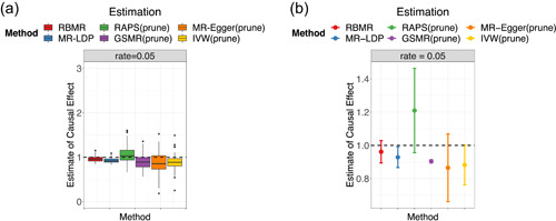
Comparisons of MR methods affected by the LD and pleiotropy. (a) Boxplot and (b) point estimates and 95% confidence intervals. LD, linkage disequilibrium; MR, Mendelian randomization

Figure 2.

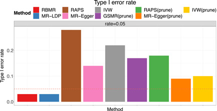
Comparisons of the type I error rates for MR methods affected by the LD and pleiotropy. LD, linkage disequilibrium; MR, Mendelian randomization

Table 1.

Comparisons of the point estimates in the terms of bias%, RMSE%, and the coverage probabilities

Method	$\widehat{\beta }$	Bias%	RMSE%	Cover%
RBMR	0.962	−3.837	7.583	94.000
MR‐LDP	0.929	−7.107	8.834	86.000
GSMR (prune)	0.905	−9.549	18.728	5.000
RAPS (prune)	1.210	20.981	155.223	87.000
MR‐Egger (prune)	0.865	−13.484	27.689	86.000
IVW (prune)	0.882	−11.768	19.996	73.000

Abbreviation: RMSE, root mean square error.

4. REAL DATA ANALYSIS

In this section, we analyzed four real data sets to demonstrate the performance of our proposed method. The 1000 Genome Project Phase 1 (1KGP) is used as the reference panel to compute the LD matrix (The 1000 Genomes Project Consortium, 2012). We first analyze two benchmark data sets commonly used for method comparison purpose, then we will estimate the causal effect of coronary artery disease (CAD) on the risk of critically ill COVID‐19 outcomes defined as those who end up on respiratory support or die from COVID‐19. We also estimate the causal effect of low‐density lipoprotein (LDL) cholesterol on the risk of Alzheimer's disease.

The first benchmark data analysis is based on the summary‐level data sets from two nonoverlapping GWAS studies for the coronary artery disease (CAD), usually referred to as the CAD‐CAD data. The true causal effect should be exactly one. The selection data set is from the Myocardial Infarction Genetics in the UK Biobank, the exposure data is from the Coronary Artery Disease (C4D) Genetics Consortium (Coronary Artery Disease (C4D) Genetics Consortium, 2011), and the outcome data is from the transatlantic Coronary Artery Disease Genome Wide Replication and Meta‐analysis (CARDIoGRAM) (Schunkert et al., 2011). We first filter the genetic variants using the selection data under different association $p$‐value thresholds ($p$‐value $\le 1\times 10^{-4},5\times 10^{-4},1\times 10^{-3}$). Then we applied our proposed RBMR method and the MR‐LDP to all the selected and possibly correlated SNPs by accounting for the LD structure explicitly. We applied the GSMR, IVW, MR‐Egger and MR‐RAPS methods using the independent SNPs after LD pruning at the LD threshold 0.05. We obtain causal effect point estimates and the corresponding 95% confidence intervals (CI) as shown in Figure 3a. We found that our proposed RBMR method outperforms other methods because it has the smallest bias and shortest confidence intervals for a range of $p$‐value thresholds. Our proposed method RBMR used all selected SNPs (without LD pruning) in the selection data set and thus we might obtain more accurate causal effect estimate. However, other methods might be biased due to the pruning process, because the pruning process might filter out the “good” IVs and keep the “bad” IVs.

Figure 3.

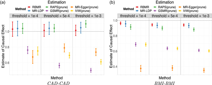
The results of CAD‐CAD and BMI‐BMI using 1KGP as the reference panel with shrinkage parameter $\lambda =0.15$. The SNPs are selected at the three thresholds ($p$‐value $\le 1\times 10^{-4},5\times 10^{-4},1\times 10^{-3}$). (a) point estimates and 95% confidence intervals of CAD‐CAD, (b) point estimates and 95% confidence intervals of BMI‐BMI. BMI, body mass index; CAD, coronary artery disease; SNP, single‐nucleotide polymorphism

To further investigate the performance of our proposed RBMR method, we consider the case that both the exposure and outcome are body mass index (BMI). We select SNPs based on previous research (Locke et al., 2015). The exposure is the BMI for physically active men and the outcome is the BMI for physically active women, both are of European ancestry (https://portals.broadinstitute.org/collaboration/giant/index.php/GIANT_consortium_data_files#2018_GIANT_and_UK_BioBank_Meta_Analysis_for_Public_Release). The point estimates and the corresponding 95% confidence intervals are shown in Figure 3b. We found that our proposed RBMR method has smaller bias than other competing methods. More numerical results are provided in the Supplementary Materials.

We apply our proposed RBMR method together with other competing methods to estimate the causal effect of CAD on the risk of critically ill coronavirus disease 2019 (COVID‐19) defined as those who end up on respiratory support or die from COVID‐19. Specifically, the selection data set is the Myocardial Infraction Genetics in the UK Biobank and the exposure data set is from Coronary Artery Disease (C4D) Genetics Consortium (2011). The outcome is obtained from Freeze 5 (January 2021) of the COVID‐19 Host Genetics Initiative (COVID‐19 HGI) Genome‐Wide Association Study (COVID‐19 Host Genetics Initiative, 2020) (https://www.covid19hg.org/results/). The data combines the genetic data of 49562 patients and two million controls from 46 studies across 19 countries (COVID‐19 Host Genetics Initiative, 2021). We mainly consider the GWAS data on the 6179 cases with critical illness due to COVID‐19 and 1483780 controls from the general populations in our analysis. We use the selection data with $p$‐value $\le 1\times 10^{-4}$ threshold to select genetic variants as IVs. As shown in Figure 4, we found a significant effect of CAD on the risk of critically ill COVID‐19 using our RBMR method ($\widehat{\beta }=0.261$ , $p$‐value = 0.008, 95$\%$ CI = [0.067, 0.454]), MR‐LDP ($\widehat{\beta }=0.258$, $p$‐value = 0.009, 95$\%$ CI = [0.065, 0.452]), GSMR ($\widehat{\beta }=0.201$, $p$‐value = 0.045, 95$\%$ CI = [0.004, 0.398]), MR‐Egger ($\widehat{\beta }=0.313$, $p$‐value = 0.036, 95% CI = [0.020, 0.605]) and IVW ($\widehat{\beta }=0.201$, $p$‐value = 0.045, 95% CI = [0.005, 0.397]). However, the result of GSMR ($\widehat{\beta }=0.268$, $p$‐value = 0.073, 95$\%$ CI = [−0.025, 0.561]) is not significant ($p$‐value $>$ 0.05). Our RBMR is more accurate as its confidence interval is slightly shorter and its $p$‐value is more significant.

Figure 4.

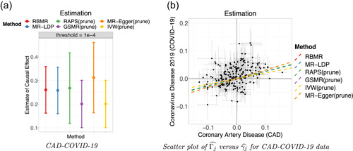
The results of CAD‐COVID‐19 using 1KGP as the reference panel with shrinkage parameter $\lambda =0.1$. The 220 SNPs are selected at the threshold ($p$‐value $\le 1\times 10^{-4}$). Each point of the scatter plot is augmented by the standard errors of $\widehat{{\mathrm{\Gamma }}_j}$ on the vertical and horizontal sides respectively. Dashed lines are the slopes fitted by the six methods. (a) point estimates and 95% confidence intervals, (b) scatter plot. CAD, coronary artery disease; SNP, single‐nucleotide polymorphism

We further apply our proposed RBMR and other competing methods to estimate the causal effect of LDL cholesterol on the risk of Alzheimer's disease. The selection data set is from Teslovich et al. (2010) with 95454 individuals, and the exposure data set is from Willer et al. (2013) with 188577 individuals. The outcome data set is obtained from the stage 1 meta‐analysis of four GWAS samples (n = 54,612) of the International Genomics of Alzheimer's Project (Lambert et al., 2013). We select the SNPs at the $p$‐value threshold $5\times 10^{-8}$. The results are summarized in Figure 5. We find that the causal effect of RBMR is $\widehat{\beta }=0.122$ ($p$‐value = $1.156\times 10^{-3}$, 95$\%$ CI = [0.048, 0.196]), the estimate of MR‐LDP is $\widehat{\beta }=0.232$ ($p$‐value = $1.242\times 10^{-3}$, 95$\%$ CI = [0.091, 0.374]) and the estimate of RAPS is $\widehat{\beta }=0.152$ ($p$‐value = $5.506\times 10^{-7}$, 95$\%$ CI = [0.093, 0.212]). The estimates of IVW ($\widehat{\beta }=0.858$, $p$‐value = $6.648\times 10^{-7}$, 95$\%$ CI = [0.520, 1.196]) and the MR‐Egger ($\widehat{\beta }=1.472$, $p$‐value = $1.574\times 10^{-6}$, 95$\%$ CI = [0.871 2.072]) are much larger than the estimates of RBMR, MR‐LDP and RAPS. And the estimate of GSMR ($\widehat{\beta }=0.033$, $p$‐value = 0.393, 95$\%$ CI = [−0.043 0.109]) is much smaller than the estimates of RBMR, MR‐LDP, and RAPS. Since there exists obvious idiosyncratic pleiotropy in this data set, hence the estimates of IVW, MR‐Egger and GSMR are likely to be biased. Both RAPS and MR‐LDP use the normal distribution to model the direct effects which might be violated in the presence of the idiosyncratic pleiotropy as in this data set, therefore the estimates of RAPS and MR‐LDP might have upward bias.

Figure 5.

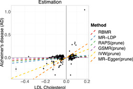
The results of LDL cholesterol on Alzheimer's disease using 1KGP as the reference panel with shrinkage parameter $\lambda =0.15$. The 292 SNPs are selected at the threshold (p‐value $\le 5\times 10^{-8}$). Each point of the scatter plot is augmented by the standard errors of $\widehat{{\mathrm{\Gamma }}_j}$ and $\widehat{{\gamma }_j}$ on the vertical and horizontal sides respectively. Dashed lines are the slopes fitted by the six methods. LDL, low‐density lipoprotein; SNP, single‐nucleotide polymorphism

5. DISCUSSION

In this paper, we propose a novel two‐sample robust MR method RBMR by accounting for the LD structure, systematic pleiotropy, and idiosyncratic pleiotropy simultaneously in a unified framework. Specifically, we propose to use the more robust multivariate generalized $t$‐distribution rather the less robust Gaussian distribution to model the direct effects of the IV on the outcome not mediated by the exposure. Moreover, the multivariate generalized $t$‐distribution can be reformulated as Gaussian scaled mixtures to facilitate the estimation of the model parameters using the parameter expanded variational Bayesian expectation‐maximum algorithm (PX‐VBEM). Through extensive simulations and analysis of two real benchmark data sets, we found that our method outperforms the other competing methods. We find that CAD might increase the risk of critically ill COVID‐19, and higher level of LDL cholesterol might increase the risk of Alzheimer's disease.

We make the following two major contributions. First, our method can account for the LD structure explicitly and thus can include more possibly correlated SNPs to reduce bias and increase estimation efficiency. Second, our RBMR method is more robust to the presence of idiosyncratic pleiotropy. This enhanced robustness can be very helpful in practice as shown by our simulation studies and real data analysis. One limitation of our proposed method is that it cannot handle correlated pleiotropy where the direct effect of the IV on the outcome might be correlated with the IV strength. We leave it as our future work.

Supporting information

Supplementary Information

Wang, A. , Liu, W. , & Liu, Z. (2022). A two‐sample robust Bayesian Mendelian Randomization method accounting for linkage disequilibrium and idiosyncratic pleiotropy with applications to the COVID‐19 outcomes. Genetic Epidemiology, 46, 159–169. 10.1002/gepi.22445

REFERENCES

- Ala‐Luhtala, J. , & Piché, R. (2016). Gaussian scale mixture models for robust linear multivariate regression with missing data. Communications in Statistics‐Simulation and Computation, 45(3), 791–813. [Google Scholar]
- Arellano‐Valle, R. B. , & Bolfarine, H. (1995). On some characterizations of the t‐distribution. Statistics & Probability Letters, 25(1), 79–85. [Google Scholar]
- Beal, M. J. (2003). Variational algorithms for approximate Bayesian inference. University of London.
- Berisa, T. , & Pickrell, J. K. (2016). Approximately independent linkage disequilibrium blocks in human populations. Bioinformatics, 32(2), 283. [DOI] [PMC free article] [PubMed] [Google Scholar]
- Blei, D. M. , Kucukelbir, A. , & McAuliffe, J. D. (2017). Variational inference: A review for statisticians. Journal of the American Statistical Association, 112(528), 859–877. [Google Scholar]
- Bound, J. , Jaeger, D. A. , & Baker, R. M. (1995). Problems with instrumental variables estimation when the correlation between the instruments and the endogenous explanatory variable is weak. Journal of the American Statistical Association, 90(430), 443–450. [Google Scholar]
- Bowden, J. , Davey Smith, G. , & Burgess, S. (2015). Mendelian randomization with invalid instruments: Effect estimation and bias detection through Egger regression. International Journal of Epidemiology, 44(2), 512–525. [DOI] [PMC free article] [PubMed] [Google Scholar]
- Burgess, S. , Butterworth, A. , & Thompson, S. G. (2013). Mendelian randomization analysis with multiple genetic variants using summarized data. Genetic Epidemiology, 37(7), 658–665. [DOI] [PMC free article] [PubMed] [Google Scholar]
- Cheng, Q. , Yang, Y. , Shi, X. , Yeung, K.‐F. , Yang, C. , Peng, H. , & Liu, J. (2020). MR‐LDP: A two‐sample Mendelian randomization for GWAS summary statistics accounting for linkage disequilibrium and horizontal pleiotropy. NAR Genomics and Bioinformatics, 2(2), lqaa028. [DOI] [PMC free article] [PubMed] [Google Scholar]
- Coronary Artery Disease (C4D) Genetics Consortium . (2011). A genome‐wide association study in Europeans and South Asians identifies five new loci for coronary artery disease. Nature Genetics, 43(4), 339. [DOI] [PubMed] [Google Scholar]
- COVID‐19 Host Genetics Initiative . (2020). The covid‐19 host genetics initiative, a global initiative to elucidate the role of host genetic factors in susceptibility and severity of the SARS‐COV‐2 virus pandemic. European Journal of Human Genetics, 28(6), 715. [DOI] [PMC free article] [PubMed] [Google Scholar]
- COVID‐19 Host Genetics Initiative . (2021). Mapping the human genetic architecture of covid‐19 by worldwide meta‐analysis. MedRxiv.
- Dai, M. , Ming, J. , Cai, M. , Liu, J. , Yang, C. , Wan, X. , & Xu, Z. (2017). IGESS: A statistical approach to integrating individual‐level genotype data and summary statistics in genome‐wide association studies. Bioinformatics, 33(18), 2882–2889. [DOI] [PMC free article] [PubMed] [Google Scholar]
- Dempster, A. P. , Laird, N. M. , & Rubin, D. B. (1977). Maximum likelihood from incomplete data via the em algorithm. Journal of the Royal Statistical Society: Series B (Methodological), 39(1), 1–22. [Google Scholar]
- Ebrahim, S. , & Smith, G. D. (2008). Mendelian randomization: Can genetic epidemiology help redress the failures of observational epidemiology? Human Genetics, 123(1), 15–33. [DOI] [PubMed] [Google Scholar]
- Ehret, G. B. , Munroe, P. B. , Rice, K. M. , Bochud, M. , Johnson, A. D. , Chasman, D. I. , Smith, A. V. , Tobin, M. D. , Verwoert, G. C. , Hwang, S. J. , Pihur, V. , Vollenweider, P. , O'Reilly, P. F. , Amin, N. , Bragg‐Gresham, J. L. , Teumer, A. , Glazer, N. , Launer, J. , Zhao, J. H. , … Johnson, T (2011). Genetic variants in novel pathways influence blood pressure and cardiovascular disease risk. Nature, 478(7367), 103–109. [DOI] [PMC free article] [PubMed] [Google Scholar]
- Evans, D. M. , Brion, M. J. A. , Paternoster, L. , Kemp, J. P. , McMahon, G. , Munafò, M. , Whitfield, J. B. , Medland, S. E. , Montgomery, G. W. , Timpson, N. J. , St. Pourcain, B. , Lawlor, D. A. , Martin, N. G. , Dehghan, A. , Hirschhorn, J. , & Smith, G. D. (2013). Mining the human phenome using allelic scores that index biological intermediates. PLoS Genetics, 9(10):e1003919. [DOI] [PMC free article] [PubMed] [Google Scholar]
- Evans, D. M. , & DaveySmith, G. (2015). Mendelian randomization: New applications in the coming age of hypothesis‐free causality. Annual Review of Genomics and Human Genetics, 16, 327–350. [DOI] [PubMed] [Google Scholar]
- Frahm, G. (2004). Generalized elliptical distributions: Theory and applications (PhD thesis). Universitätsbibliothek.
- Hansen, C. , Hausman, J. , & Newey, W. (2008). Estimation with many instrumental variables. Journal of Business & Economic Statistics, 26(4), 398–422. [Google Scholar]
- Hemani, G. , Zheng, J. , Wade, K. H. , Laurin, C. , Elsworth, B. , Burgess, S. , Bowden, J. , Langdon, R. , Tan, V. , Yarmolinsky, J. , Shihab, H. A. , Timpson, N. J. , Evans, D. M. , Relton, C. , Martin, R. M. , Smith, G. D. , Gaunt, T. R. , & Haycock, P. C. (2016). MR‐Base: A platform for systematic causal inference across the phenome using billions of genetic associations. BioRxiv, 078972. [Google Scholar]
- Kotz, S. , & Nadarajah, S. (2004). Multivariate T‐distributions and their applications. Cambridge University Press. [Google Scholar]
- Lambert, J. C. , Ibrahim‐Verbaas, C. A. , Harold, D. , Naj, A. C. , Sims, R. , Bellenguez, C. , DeStafano, A. L. , Bis, J. C. , Beecham, G. W. , Grenier‐oley, B. , Russo, G. , Thorton‐Wells, T. A. , Jones, N. , Smith, A. V. , Chouraki, V. , Thomas, C. , Ikram, M. A. , Zelenika, D. , Vardarajan, B. N. , … Amouyel, P. (2013). Meta‐analysis of 74,046 individuals identifies 11 new susceptibility loci for Alzheimer's disease. Nature Genetics, 45(12), 1452–1458. [DOI] [PMC free article] [PubMed] [Google Scholar]
- Lawlor, D. A. , Harbord, R. M. , Sterne, J. A. , Timpson, N. , & DaveySmith, G. (2008). Mendelian randomization: Using genes as instruments for making causal inferences in epidemiology. Statistics in Medicine, 27(8), 1133–1163. [DOI] [PubMed] [Google Scholar]
- Liu, C. , Rubin, D. B. , & Wu, Y. N. (1998). Parameter expansion to accelerate EM: The PX‐EM algorithm. Biometrika, 85(4), 755–770. [Google Scholar]
- Locke, A. E. , Kahali, B. , Berndt, S. I. , Justice, A. E. , Pers, T. H. , Day, F. R. , Powell, C. , Vedantam, S. , Buchkovich, M. L. , Yang, J. , Croteau‐Chonka, D. C. , Esko, T. , Fall, T. , Ferreira, T. , Gustafsson, S. , Kutalik, Z. , Luan, J. , Mägi, R. , Randall, J. C. … Speliotes, E. K. (2015). Genetic studies of body mass index yield new insights for obesity biology. Nature, 518(7538), 197–206. [DOI] [PMC free article] [PubMed] [Google Scholar]
- MacArthur, J. , Bowler, E. , Cerezo, M. , Gil, L. , Hall, P. , Hastings, E. , Junkins, H. , McMahon, A. , Milano, A. , Morales, J. , Pendlington, Z. M. , Welter, D. , Burdett, T. , Hindorff, L. , Flicek, P. , Cunningham, F. , & Parkinson, H. (2017). The new NHGRI‐EBI Catalog of published genome‐wide association studies (GWAS catalog). Nucleic Acids Research, 45(D1), D896–D901. [DOI] [PMC free article] [PubMed] [Google Scholar]
- Martens, E. P. , Pestman, W. R. , de Boer, A. , Belitser, S. V. , & Klungel, O. H. (2006). Instrumental variables: Application and limitations. Epidemiology, 17, 260–267. [DOI] [PubMed] [Google Scholar]
- Pickrell, J. K. , Berisa, T. , Liu, J. Z. , Ségurel, L. , Tung, J. Y. , & Hinds, D. A. (2016). Detection and interpretation of shared genetic influences on 42 human traits. Nature Genetics, 48(7), 709. [DOI] [PMC free article] [PubMed] [Google Scholar]
- Purcell, S. , Neale, B. , Todd‐Brown, K. , Thomas, L. , Ferreira, M. A. , Bender, D. , Maller, J. , Sklar, P. , De Bakker, P. I. , Daly, M. J. , & Sham, P. C. (2007). PLINK: A tool set for whole‐genome association and population‐based linkage analyses. The American Journal of Human Genetics, 81(3), 559–575. [DOI] [PMC free article] [PubMed] [Google Scholar]
- Rothman, A. J. (2012). Positive definite estimators of large covariance matrices. Biometrika, 99(3), 733–740. [Google Scholar]
- Schunkert, H. , König, I. R. , Kathiresan, S. , Reilly, M. P. , Assimes, T. L. , Holm, H. , Preuss, M. , Stewart, A. F. , Barbalic, M. , Gieger, C. , Absher, D. , Aherrahrou, Z. , Allayee, H. , Altshuler, D. , Anand, S. S. , Andersen, K. , Anderson, J. L. , Ardissino, D. , Ball, S. G. , … Samani, N. J. (2011). Large‐scale association analysis identifies 13 new susceptibility loci for coronary artery disease. Nature Genetics, 43(4), 333–338. [DOI] [PMC free article] [PubMed] [Google Scholar]
- Solovieff, N. , Cotsapas, C. , Lee, P. H. , Purcell, S. M. , & Smoller, J. W. (2013). Pleiotropy in complex traits: Challenges and strategies. Nature Reviews Genetics, 14(7), 483–495. [DOI] [PMC free article] [PubMed] [Google Scholar]
- Teslovich, T. M. , Musunuru, K. , Smith, A. V. , Edmondson, A. C. , Stylianou, I. M. , Koseki, M. , Pirruccello, J. P. , Ripatti, S. , Chasman, D. I. , Willer, C. J. , Johansen, C. T. , Fouchier, S. W. , Isaacs, A. , Peloso, G. M. , Barbalic, M. , Ricketts, S. L. , Bis, J. C. , Aulchenko, Y. S. , Thorleifsson, G. , … Kathiresan, S. (2010). Biological, clinical and population relevance of 95 loci for blood lipids. Nature, 466(7307), 707–713. [DOI] [PMC free article] [PubMed] [Google Scholar]
- The 1000 Genomes Project Consortium . (2012). An integrated map of genetic variation from 1,092 human genomes. Nature, 491(7422), 56. [DOI] [PMC free article] [PubMed] [Google Scholar]
- Van der Vaart, A. W. (2000). Asymptotic statistics (Vol. 3). Cambridge University Press. [Google Scholar]
- Verbanck, M. , Chen, C.‐Y. , Neale, B. , & Do, R. (2018). Detection of widespread horizontal pleiotropy in causal relationships inferred from Mendelian randomization between complex traits and diseases. Nature Genetics, 50(5), 693–698. [DOI] [PMC free article] [PubMed] [Google Scholar]
- Wang, B. , & Titterington, D. (2005). Inadequacy of interval estimates corresponding to variational Bayesian approximations. In AISTATS. Citeseer.
- Willer, C. J. , Schmidt, E. M. , Sengupta, S. , Peloso, G. M. , Gustafsson, S. , Kanoni, S. , Ganna, A. , Chen, J. , Buchkovich, M. L. , Mora, S. , Beckmann, J. S. , Bragg‐Gresham, J. L. , Chang, H. Y. , Demirkan, A. , Den Hertog, H. M. , Do, R. , Donnelly, L. A. , Ehret, G. B. , Esko, T. , … Abecasis, G. R (2013). Discovery and refinement of loci associated with lipid levels. Nature Genetics, 45(11), 1274–1283. [DOI] [PMC free article] [PubMed] [Google Scholar]
- Yang, Y. , Dai, M. , Huang, J. , Lin, X. , Yang, C. , Chen, M. , & Liu, J. (2018). LPG: A four‐group probabilistic approach to leveraging pleiotropy in genome‐wide association studies. BMC Genomics, 19(1), 503. [DOI] [PMC free article] [PubMed] [Google Scholar]
- Yang, Y. , Shi, X. , Jiao, Y. , Huang, J. , Chen, M. , Zhou, X. , Sun, L. , Lin, X. , Yang, C. , & Liu, J. (2020). CoMM‐S2: A collaborative mixed model using summary statistics in transcriptome‐wide association studies. Bioinformatics, 36(7), 2009–2016. [DOI] [PubMed] [Google Scholar]
- Zhao, J. , Ming, J. , Hu, X. , Chen, G. , Liu, J. , & Yang, C. (2020). Bayesian weighted Mendelian randomization for causal inference based on summary statistics. Bioinformatics, 36(5), 1501–1508. [DOI] [PubMed] [Google Scholar]
- Zhao, Q. , Wang, J. , Hemani, G. , Bowden, J. , & Small, D. S. (2020). Statistical inference in two‐sample summary‐data Mendelian randomization using robust adjusted profile score. Annals of Statistics, 48(3), 1742–1769. [Google Scholar]
- Zhu, X. , & Stephens, M. (2017). Bayesian large‐scale multiple regression with summary statistics from genome‐wide association studies. The Annals of Applied Statistics, 11(3), 1561. [DOI] [PMC free article] [PubMed] [Google Scholar]
- Zhu, Z. , Zheng, Z. , Zhang, F. , Wu, Y. , Trzaskowski, M. , Maier, R. , Robinson, M. R. , McGrath, J. J. , Visscher, P. M. , Wray, N. R , & Yang, J. (2018). Causal associations between risk factors and common diseases inferred from GWAS summary data. Nature Communications, 9(1), 224. [DOI] [PMC free article] [PubMed] [Google Scholar]
Associated Data
This section collects any data citations, data availability statements, or supplementary materials included in this article.
Supplementary Materials