Post COVID-19 pandemic recovery of intracity human mobility in Wuhan: Spatiotemporal characteristic and driving mechanism

Graphical abstract

Abstract

After successfully inhibiting the first wave of COVID-19 transmission through a city lockdown, Wuhan implemented a series of policies to gradually lift restrictions and restore daily activities. Existing studies mainly focus on the intercity recovery under a macroscopic view. How does the intracity mobility return to normal? Is the recovery process consistent among different subareas, and what factor affects the post-pandemic recovery? To answer these questions, we sorted out policies adopted during the Wuhan resumption, and collected the long-time mobility big data in 1105 traffic analysis zones (TAZs) to construct an observation matrix (A). We then used the nonnegative matrix factorization (NMF) method to approximate A as the product of two condensed matrices (WH). The column vectors of W matrix were visualized as five typical recovery curves to reveal the temporal change. The row vectors of H matrix were visualized to identify the spatial distribution of each recovery type, and were analyzed with variables of population, GDP, land use, and key facility to explain the recovery driving mechanisms. We found that the “staggered time” policies implemented in Wuhan effectively staggered the peak mobility of several recovery types (“staggered peak”). Besides, different TAZs had heterogeneous response intensities to these policies (“staggered area”) which were closely related to land uses and key facilities. The creative policies taken by Wuhan highlight the wisdom of public health crisis management, and could provide an empirical reference for the adjustment of post-pandemic intervention measures in other cities.

1. Introduction

The first wave of COVID-19 pandemic had posed serious threats to social stability and public health globally. On January 23, 2020, as one of the high-risk areas, Wuhan launched the level I public health emergency response and pressed the pause button (Lau et al., 2020). The city lockdown significantly reduced the human mobility and limited the virus transmission. However, home quarantine and production shutdown also stagnated society and economic development (Feng et al., 2021, Li et al., 2021a). After infection cases ushered in a turning point in early March, the adjustment and reduction of intervention measures became a new hotspot (Yang and Xie, 2020). Since immediate cancellation of travel restrictions and stay-at-home order would inevitably lead to an epidemic resurgence, Wuhan government has formulated a series of policies to promote the city’s resumption orderly (Lai et al., 2020, Prem et al., 2020). A study finds that the overall human mobility in Wuhan only reached 40 % of the normal level by the March end (Tian et al., 2021), which is slower than other cities in China. How does Wuhan recover eventually? Is the recovery process consistent among different subareas within this megacity? What factor affects the city recovery process? These important questions remain to be addressed. In particular, quantitatively understanding spatiotemporal characteristics and driving mechanisms of the city recovery process have reference value for crisis management and policymaking in the post-pandemic era (Barouki et al., 2021).

Human mobility, generated by people’s changing behaviors, has been considered one of the most representative indicators during the COVID-19 pandemic (Buckee et al., 2020, Chen et al., 2021, Lai et al., 2020). In order to analyze the time-varying pandemic process, real-time updated mobility data is necessary (Wu et al., 2020, Xu et al., 2021). Fortunately, many big data companies including Google, Facebook, Safegraph, Baidu, etc. have opened their Location Based Service (LBS) data from large mobile devices for scientific uses (Huang et al., 2020b). These mobility datasets provide high-resolution information about population activities and movements, which have been widely used to monitor the pandemic change and assess the effectiveness of non-pharmaceutical interventions (Grantz et al., 2020, Huang et al., 2020a, Li et al., 2021b). Many existing studies aggregate the mobility index into large spatial units (including states, counties, provinces, and cities), draw the time sequence of each unit (Wang and Noland, 2021, Xiong et al., 2020), and design various statistical indexes to describe the COVID-19 situation difference (Zhao et al., 2021a). In addition, existing studies further use Pearson correlation coefficient (Xu et al., 2020), multiple linear regression (Chen et al., 2021), geographically weighted regression (Dueñas et al., 2021, Xu et al., 2021), and geodetector (Zhao et al., 2021a) to reveal the relationship between socio-economic covariates (like population, GDP, land use) and the COVID-19 impact.

However, there are some unsolved issues in the existing studies. First, most studies take the city as a whole to analyze the COVID-19 recovery process, while few studies focus on the spatiotemporal discrepancy within a city scale (Xu et al., 2022). Second, existing studies mainly cover the partial recovery process, and a complete recovery process is quite scarce. Third, the diverse recovery types are usually classified empirically and qualitatively, which may lose some latent rules and patterns. To sum up, city, a complex synthesis, owns heterogeneous elements and different performances in terms of the pandemic issue, which urgently needs a refined observation with the long length data.

Meanwhile, efficient techniques for processing mobility data are attracting attention. For one thing, matrix organization is a useful way of assembling spatiotemporal data. Concretely, the mobility data can convert into an observation matrix by taking space units and time series as two-dimensional coordinates. For another thing, dimensionality reduction is particularly helpful in mining representative mode and simplifying problems. Among a large number of algorithms, nonnegative matrix factorization (NMF) has stood out due to its excellent properties and practical values (Liu et al., 2006). NMF approximates the matrix A by the product of two condensed matrices W and H (Objective function: $A\approx WH$). It has been widely used in image processing, genetic engineering, audio separation, and text mining (Brunet et al., 2004, Hutchins et al., 2008, Kang and Qin, 2016), and is also applied to decompose the mobility flow network between cities during the pandemic (Edsberg Mollgaard et al., 2022).

To respond the above-mentioned issues, this study takes the complete first-wave of COVID-19 pandemic in Wuhan as the research object. First, we sorted out key events and main policies to organize the recovery timeline. Then, we divided the study area into 1105 traffic analysis areas (TAZs) and collected long series mobility data from the Baidu LBS platform. Next in Fig. 1 , we constructed a nonnegative observation matrix $A_{+}$(220*1105) with time sequences as a column vector, TAZ units as a row vector, and mobility indexes as a legend. After selecting the optimal decomposition rank $k$, we decomposed two simplified matrices $W_{+}\left(220\ast k\right)$ and $H_{+}\left(k\ast 1105\right)$ through NMF. The temporal visualization of column vectors in W matrix displayed five typical recovery curves, and the spatial visualization of row vectors in H matrix showed intensity differences of each recovery type. On these bases, we used the local spatial autocorrelation method to identify the potential recovery aggregation, and we finally chose the spatial lag model to explain the driving mechanism combined with multi-source data such as population, GDP, land uses, and key facilities.

Fig. 1.

Conceptual framework of this study.

The remained contents were as follows. In the 2nd section, the study area, event timeline, data sources, and methods were provided. In the 3rd section, the NMF decomposition results were analyzed in detail. We first temporal visualized five typical recovery curves based on matrix W and verified their practical meanings by comparing with the observed time sequences. Then, we spatial visualized the occurrence intensity of each recovery type based on matrix H, and elaborated the local agglomeration and driving factors of each recovery type through spatial autocorrelation and spatial lag model. Sections 4 & 5 discussed the findings and concluded the study, respectively.

2. Materials and methods.

2.1. Study area and key events

Wuhan is the capital city of Hubei Province in China. Its built-up area is 1217 km²and resident population is 11.08 million in 2020. On January 23, 2020, Wuhan was locked down to deal with the severe epidemic situation. This lockdown directly impacted human mobility and effectively controlled the COVID-19 spread (Huang et al., 2021). After the infection cases continuously decreased, Wuhan implemented a series of policies to gradually withdraw the intervention measures and orderly promote the resumption of work and production (http://wjw.wuhan.gov.cn/). Fig. 2 a marked the key dates corresponding to Table 1 . It can be seen that the lockdown greatly limited citizen mobility, and the implementation of recovery policies contributed to the mobility growth. We defined early September in 2020 as the end of this COVID-19 wave since its mobility counts reached the pre-pandemic level.

Fig. 2.

Daily mobility counts and study area map.

Table 1.

Timeline of key events during the COVID-19 pandemic in Wuhan.

Date	Events	Details
2020/01/23	City locked down (internal and external traffic closure)	Level I public health emergency response was launched. City locked down from 10 a.m. Public transportation stopped, cross-river tunnels closed, and motor vehicles controlled.
2020/02/10	Home quarantine. Government participated in community epidemic prevention and disinfection	Residential communities were closed. Staffs of government agencies participated in community epidemic prevention (household symptom survey). Thorough disinfection carried out. Generally, people shall not leave home except for medical treatment and epidemic prevention works.
2020/03/11	Phase one reopening	The arrangement for work resumption began. Industries ensuring epidemic prevention, contributing to important national economy and people’s livelihood given the priority to resume.
2020/03/28	Phase two reopening	Internal traffic (public transportation) and enter-city traffic partial resumed. Government staffs returned to normal work.
2020/04/08	City lifted lockdown	Wuhan officially reopened. External traffic resumed. Public transportation fully operated.
2020/08/08	Phase three reopening	“Huiyou Hubei” incentive policy was implemented: all A-level scenic spots were free for tickets to tourists all over the country.
2020/09/05	Phase four reopening	Students in different provinces and cities returned to school.

In order to analyze the spatial difference of intracity recovery process, we divided the study area into 1105 traffic analysis zones (TAZs). In Fig. 2b, the main city which consists of three towns (Hankou, Hanyang, and Wuchang) was marked in orange color. Around the main city is twenty functional areas: Yangluo and Beihu are dominated by heavy chemical industry and port transportation; Baoxie and Liufang mainly contain optoelectronics, biomedicine and other high-tech industries; Qingling, Huangjiahu, Zhifang, and Zhengdian are organized to be educational and scientific research parks and modern logistics bases; Changfu and Xuefeng mainly contain automobile industries and logistics; Caidian, Wujiashan, and Jinyinhu are dominated by food processing, modern logistics and light industry; Panlong, Hengdian, and Wuhu take advantage of Tianhe Airport to form centralized air transportation and airport industry.

2.2. Data collecting and processing

According to the statistical bulletin of communication industry in 2020 (https://www.miit.gov.cn/), the total number of smartphone users in China has reached 1.289 billion. As the largest Internet company in China, Baidu covers about 86.2 % of the application (APP) market (https://www.questmobile.com.cn/). When users access Baidu APPs (such as Baidu search, Baidu map, Baidu weather, etc.) through smartphones, Their anonymous location (longitude and latitude) will be recorded in real time after consent (Li et al., 2019). With advanced positioning technology, the mobility data from Baidu not only has overwhelming population penetration and coverage, but also has high recording accuracy (Zhou et al., 2022).

Based on the Location Based Service (LBS) mobility data, Baidu further designed a visual product (Baidu heat map) in 2011. This product is updated every 15 min, which can be used to track and analyze the dynamic information of population activities. In the Baidu heat map, Wuhan has been pre-divided into continuous geographic grids (150 m*150 m). The total number of recorded locations falling into each geographic grid will be regarded as the population heat count on the grid (Wu et al., 2021). Then, according to the preset unified classification standard, the population heat counts are automatically converted into the population heat index ranging from 0 to 100. Spatially, the population heat indexes will be rendered with a red–greenblue color gradient (Zhou et al., 2020). It should be noted that only when the spatial displacement of a person exceeds the distance threshold (50 m) within 15 min, the recorded location will be counted and mapped. Therefore, the heat index does not reflect the population numbers, but can accurately show the human mobility change in geographical space (Zhao et al., 2021a). We denote it as the human mobility index in the remaining part. This data source has already been used in population aggregation detection, urban functional zoning, transportation field research, and COVID-19 related analysis (Chen et al., 2021, Huang et al., 2021, Li et al., 2021b, Lyu and Zhang, 2019, Zhao et al., 2021a).

In this study, we focused on comparing the human mobility index over multiple days from the city lockdown (late January) to the university reopening (early September). We collected the hourly human mobility index and then used ArcGIS software to derive the daily human mobility index. As shown in Fig. 3 a, the human mobility index was quite low during the city lockdown, meaning that few human mobilities exceed the recognizable distance threshold. Moreover, significant differences in human mobility indexes occurred during different recovery stages. We also conducted essential pretreatments as follows: (1) a simple moving average method with 7 days window was applied to smooth the sequence and reduce small-scale disturbances; (2) maximum and minimum values of each TAZ’s sequence were extracted to normalize and limit the mobility range into [0,1] which solved the incompatibility caused by various population bases in different TAZs; (3) an observation matrix $A_{+}$(220*1105) was defined with column $N\in \left[1,220\right]$ represented the time sequence, row $M\in \left[1,1105\right]$ displayed the TAZ ID, and legend $\in \left[0,1\right]$ reflected the normalized human mobility index (as shown in Fig. 3b).

Fig. 3.

Baidu heat maps of key dates and observation matrix of human mobility indexes Notes. A unified grading standard was applied in part a to compare the human mobility index over multiple days.

Other data were all provided by Wuhan Geomatics Institute (http://www.whkc.com/). The resident population (POP) and GDP were 250 m grids, and we calculated their density on each TAZ by the zonal statistic method. The land use data was extracted from the Third National Land Survey, and it was a kind of refined patches combining the computer interpretation and manual supervision technology. The land uses were produced in December 2018, and details of the land classification can be seen on the official website (http://www.mnr.gov.cn/). The point of interest (POI) data was collected from Baidu map in June 2019 (https://lbs.baidu.com/).

2.3. Quantitative methods

2.3.1. Nonnegative matrix factorization

In Fig. 3b, we defined the observation matrix $A_{+}\left(220\ast 1105\right)$, whose column vector was time sequence, row vector was space sequence, and legend was the normalized human mobility index. For example, the m-th column represents the recovery curve of the m-th TAZ in time sequence. Our target is to find several typical recovery types with which any TAZ time sequence can be built via a positive linear combination. In this study, nonnegative matrix factorization (NMF) was applied, since this method can effectively discover the hidden patterns of large-volume data and show the interpretable decomposition results based on retaining nonnegative characteristics (Monselise et al., 2021).

Given a decomposition rank $k$ in advance, the NMF method can search two nonnegative matrices $W_{+}\left(220\ast k\right)$ and $H_{+}\left(k\ast 1105\right)$ to approximate $A\approx WH$. Specifically, the elements $a_{\mathit{ij}}$ in the matrix $A$ is the weighted sum of i-row vector in the left matrix $W$ (also known as the coefficient matrix), and the weight is the element of j-column vector in the right matrix $H$ (also known as the dictionary matrix) (Kang and Qin, 2016). In this study, the $W$ matrix corresponds to k typical recovery types, and the H matrix represents the weight value (occurrence intensity) of each recovery type on different TAZs.

Mathematically, the method initializes matrices $W$ and $H$ randomly and iterates to achieve the minimum divergence function D. In the process, $W$ and $H$ are updated by coupling the Divergence Equation:

$$D=\sum _{i,j}A{}_{i,j}\log (A{}_{i,j}/{(WH)}_{i,j})-A{}_{i,j}+{(WH)}_{i,j}$$

$$W_{\mathit{ia}}\leftarrow \frac{W_{\mathit{ia}}}{{\sum }_k{W}_{\mathit{ka}}}\left(\sum _u{H}_{\mathit{au}}\frac{A_{\mathit{iu}}}{{(WH)}_{\mathit{iu}}}\right)H_{\mathit{au}}\leftarrow \frac{H_{\mathit{au}}}{{\sum }_v{H}_{\mathit{av}}}\left(\sum _i{W}_{\mathit{ia}}\frac{A_{\mathit{iu}}}{{(WH)}_{\mathit{iu}}}\right)$$

Where the fidelity of the approximation enters the updates through the quotient $A_{\mathit{iu}}/{(WH)}_{\mathit{iu}}$. Monotonic convergence can be proven using techniques similar to those proving the convergence of the EM algorithm. The update rules preserve the non-negativity and constrain the column sum to unity of $W$ and $H$. This sum constraint is a convenient way of eliminating the degeneracy associated with the invariance of $\mathit{WH}$ under the transformation $W\to W\mathrm{\Lambda }$ and $\mathrm{H}\to \mathrm{H}\mathrm{\Lambda }$ ($\mathrm{\Lambda }$ is a diagonal matrix) (Brunet et al., 2004).

Particularly, the decomposition rank $k$ is a key parameter of NMF. There are two common selection criteria, including cophenetic correlation coefficient (Brunet et al., 2004) and residual sum of squares (RSS) (Hutchins et al., 2008). In the latter one, the RSS criterion ${\Vert A-WH\Vert }_F^2$ (F represents Frobenius norm) between the observation matrix $A$ and the NMF-estimated matrix $\mathit{WH}$ provides a natural method for estimation of $k$. As shown in Fig. 4 , we tested the RSS with k ∈ [2,10]. At first, RSS decreased sharply with the increase of $k$, meaning that the increased rank effectively reduced the information loss and captured the hidden patterns in the observation matrix. When $k$ = 5, the figure showed an inflection point. When $k$ continued to increase, the additional reduction of RSS was less, meaning that the increased rank only captured the random noise. Therefore, we chose $k$ = 5 as the optimal decomposition rank.

Fig. 4.

Selection of the best decomposition rank..$\mathit{k}$

2.3.2. Global and local spatial autocorrelation

In this study, we hoped to find the main occurrence areas of each recovery type. But the recovery intensity of different geographic TAZs might not be independent. The shorter spatial distance of TAZs means a stronger potential correlation, which is called spatial autocorrelation. The global Moran’s I index is commonly adopted to measure the average degree of this kind of correlation. The domain of this index ranges from −1 to 1. Particularly, if it is great than 0, the similar observation values tend to cluster together (for example, high values cluster around other high values).

$$I=\frac{n}{S_0}\ast \frac{{\sum }_{i=1}^n{\sum }_{j=1}^n{w}_{\mathit{ij}}\left(h_i-\overline{h}\right)\left(h_j-\overline{h}\right)}{{\sum }_{i=1}^n{\left(h_i-\overline{h}\right)}^2}$$

where $I$ is the global Moran’s I index; $n$ is the total number of TAZs; $w_{\mathit{ij}}$ is the spatial weight between TAZ i and TAZ j, $S_0={\sum }_{i=1}^n{\sum }_{j=1}^n{w}_{\mathit{ij}}$ is the aggregation of spatial weights; $h_i$ and $h_j$ denote the recovery intensity of TAZ i and TAZ j, respectively. $\overline{h}$ is the mean intensity of all observations.

The global Moran’s I only reflects whether clusters exist in the study area, and it cannot indicate where these clusters appear specifically. Therefore, the Local Indicators of Spatial Association (LISA) has been adopted to test local clusters of the recovery intensity and visualize these clusters spatially (Anselin et al., 2006, Ord and Getis, 1995).

$$I_i={(h}_i-\overline{h})\sum _j^n{w}_{\mathit{ij}}{(h}_j-\overline{h})$$

Where $I_i$ is the local Moran’s I index of TAZ $i$, whose range is not limited from −1 to 1. Instead, it took a four-quadrant rule to define clusters. ${(h}_i-\overline{h})$ compares the observation values of the TAZ $i$ with the average value of the whole study area, and the ${\sum }_j^n{w}_{\mathit{ij}}{(h}_j-\overline{h})$ compares the observation values of other surrounding TAZs with the average value of the whole region. Take 0 as the threshold, LISA can divide these differences into four clusters: high-high, high-low, low–high and low-low. For example, if the ${(h}_i-\overline{h})$ and ${\sum }_j^n{w}_{\mathit{ij}}{(h}_j-\overline{h})$ both are greater than 0, TAZ $i$ will be considered into “high-high” cluster (hot spot). Similarly, “low-low” represents low value aggregations (cold spots). In particular, “high-low” indicates that the TAZ $i$ itself has high value but its nearby TAZs have low values. Conversely, “low-high” indicates that the TAZ $i$ has low value but surrounded by high values.

In this study, we adopted the first-order inverse distance to form the spatial weight matrix:

$$w_{\mathit{ij}}=\left\{\begin{array}{c}1/d_{\mathit{ij}},i\ne j\\ 0,i=j\end{array}\right)$$

Where $w_{\mathit{ij}}$ is the spatial weight between i-th and j-th TAZs; $d_{\mathit{ij}}$ is the Euclidean distance from the centroid of TAZ i to that of TAZ j.

2.3.3. Spatial lag regression and spatial error regression

Given that we wanted to understand the driving mechanism of the built environment for different recovery types, we took the occurrence intensity of each recovery type as the dependent variable. Nevertheless, a conventional linear regression $y=\beta X+\epsilon$ cannot account for the spatial autocorrelation of the recovery intensity. Therefore, two classical spatial econometric models were applied in this study. (1) Spatial lag model (SLM). SLM adds a spatial lag term $\rho Wy$ into the regression equation to consider the proximity effect, that is, the recovery intensity on the peripheral units has an effect on the central unit. (2) Spatial error model (SEM). SEM adds a spatial error term $\lambda W\epsilon$ to consider the structural effect, that is, the spatial autocorrelation between adjacent units is mainly presented in the error term of the linear regression (Wen et al., 2011).

$$y=\rho Wy+\beta X+\epsilon$$

$$\epsilon =\lambda W\epsilon +\mu$$

Where $y$ is the recovery intensity, and $X$ is the independent variable matrix. $\beta$ is the parameter vector to be estimated. $W$ is the inverse distance spatial weight matrix. $\epsilon$ is the model error term with $\mu N(0,{\sigma }^{2}I)$. $\rho$ is the spatial correlation coefficient, which indicates the strength of the proximity effect. $\lambda$ is the spatial autoregression coefficient. The larger the $\left|\lambda \right|$, the greater the structural effect. For SLM, $\lambda =0$. For SEM, $\rho =0$. If $\rho =0$ and $\lambda =0$, the formula becomes the standard linear regression (OLS) model.

To judge which model is appropriate, we applied a progressive estimation method based on the Lagrange multiplier (LM) (Anselin et al., 1996). (1) Set $\rho =0$ and $\lambda =0$ (OLS model), then test the Moran’s I of the residual term $\epsilon$. If $P_{\mathit{value}}<0.05$, the spatial autocorrelation should be considered. (2) Apply LM tests for SLM and SEM. For LM-lag test, H0: set $\lambda =0$ and assume $\rho =0$. If $P_{\mathit{value}}<0.05$, then there exists significant proximity effect. For LM-error test, H0: set $\rho =0$ and assume $\lambda =0$. If $P_{\mathit{value}}<0.05$, then there exists significant structural effect. (3) If both LM tests are significant, then apply the Robust LM tests. For Robust LM-lag test, H0: after correcting the structural effect, assume $\rho =0$. If $P_{\mathit{value}}<0.05$, the proximity effect is dominant and SLM should be applied. For Robust LM-error test, H0: after correcting the proximity effect, assume $\lambda =0$. If $P_{\mathit{value}}<0.05$, the structural effect is dominant and SEM should be applied. (4) If both Robust LM tests are rejected, the model with a high Robust LM value should be applied.

3. Results

In Fig. 5a, we counted the human mobility indexes of 1105 TAZs in 220 consecutive days and defined the nonnegative observation matrix $A_{+}\left(220\ast 1105\right)$. It can be seen that these diverse TAZ recovery curves were hard to directly extract potential patterns. Therefore, we adopted the NMF method to determine typical recovery curves. As shown in Fig. 5b and Fig. 5c, we chose $k=5$ as the optimal decomposition rank and decomposed the observation matrix into a coefficient matrix $W_{+}\left(220\ast 5\right)$ and a dictionary matrix $H_{+}\left(5\ast 1105\right)$. The column vectors of the $W$ matrix indicated five decomposed time sequence, which corresponds to five typical recovery types named TYPE 1 ∼ 5. In the process of matrix multiplication, the population mobility index of n-th row & m-th column (in the observation matrix) was the inner product of the n-row vector in W matrix and the m-th column vector in H matrix, that is, $A\left(n,m\right)={\sum }_{k=1}^{5}W\left(n,k\right)H(k,m)$. $H(k,m)$ represented the weight value (occurrence intensity) of TYPE-k recovery on m-th TAZ. Therefore, the row vectors of the $H$ matrix represented the intensity of each recovery TYPE among different TAZs.

Fig. 5.

Nonnegative matrix factorization results.

The rest of this section first visualized the time sequence of each mobility recovery type and verified its correctness. Then we visualized the occurrence intensity of each recovery type in space, and discussed its potential spatial agglomeration and driving mechanism:

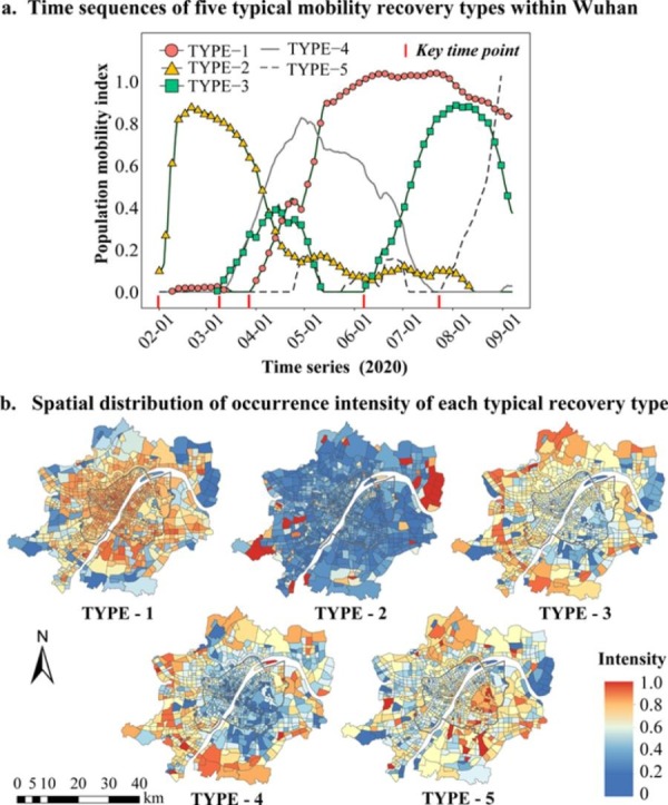
3.1. Time sequences of five typical type of population mobility recovery

According to the coefficient matrix ${\mathit{W}}_{+}\left(220\mathbf{\ast }5\right)$ ( Fig. 6a), we visualized the typical time sequence of each recovery type and marked key dates through red dots on the X-axis ( Fig. 6b). After ranking the intensity of each recovery type (Fig. 5 c), we visualized the observed time sequences of the top five TAZs of each category (Fig. 6c) to verify the practical meaning of our typical recovery type.

Fig. 6.

Comparison between the typical recovery types and observed time sequences.

Specifically, TYPE-1 followed S-shape which started to recover from the partial reopening of public transportation (March 28) and tended to be stable after early June (Fig. 6b). TYPE-2 maintained a high mobility level during the city lockdown (from late January to early April). TYPE-5 increased exponentially since late July and fully restored within one month. The observed recovery sequences of TYPE-1, TYPE-2 and TYPE-5 well matched our typical recovery types (Fig. 6c). It is worth noting that the TAZs of TYPE-2 only maintained a large population mobility between February and April, which meant the TYPE-2 undertook important functions during the urban lockdown and gradually disappeared after the city reopening.

On March 11, Wuhan government issued the arrangement for work and production to resume. This policy held that key industries ensuring epidemic prevention, contributing to important national economy and people’s livelihood should be given the resumption priority. The NMF method effectively separated these recovery curves of ordinary industries (TYPE-3) and key industries (TYPE-4) in Fig. 6b. Among them, our typical time sequence of TYPE-4 could well capture the process of fully recovery from early March to early May. Particularly, the observed recovery sequences of TYPE-4 decreased rapidly by 0.2 and turned into a continuous slow growth (Fig. 6c). Due to the trend of continuous slow growth was similar to TYPE-1, it is not reflected in our TYPE-4 typical curve. Instead, the NMF automatically supplemented the trend of the steep decline (red dotted line). Therefore, these observed sequences of TYPE-4 were linear combinations of TYPE-1 and TYPE-4 typical curves. The typical TYPE-4 curve could represent a kind of unique mobility recovery and accurately answer its start time, degree and speed of mobility growth.

In Fig. 6b, the typical recovery of TYPE-3 had two phases: phase I was from early March to early May when the human mobility index restored less than half; phase II was from early June to early August when the human mobility index restored fully. As shown in Fig. 6c, the observed sequences of TYPE-3 seemed partially similar to TYPE-1 and TYPE-4. However, this kind of sequence increased in early March earlier than TYPE-1, expressed a short decline and slope change at the beginning of April different from TYPE-3, and had another rapid growth at the beginning of July. Our typical curve of TYPE-3 recorded these distinctive changes and automatically supplements the trend line (red dotted line). Therefore, these observed sequences of TYPE-3 contained the typical trend of TYPE-1 and TYPE-4, but we could not ignore that the TYPE-3 typical recovery also existed in specific periods from March to May and from July to August.

To sum up, we successfully decomposed the complex observation curves into five typical recovery types. Except for the phase II recovery of TYPE-3 was from half to full between July and August, our typical curves could well answer when the mobility recovery starts, to what extent, and at what speed.

3.2. Spatial distribution and local autocorrelation of the intensity of each mobility recovery type

As mentioned previously, in dictionary matrix ${\mathit{H}}_{+}\left(5\mathbf{\ast }1105\right)$ (Fig. 7 a), $H(k,m)$ represented the weight value (occurrence intensity) of TYPE-k recovery on m-th TAZ. Through the comparison of the k-row vector in H matrix, we observed that the TYPE-k intensity was different among different TAZs. The higher k-row value meant a closer similarity to the TYPE-k recovery. In other words, the TYPE-k recovery was more likely to occur in those TAZs with high intensity. In Fig. 7b, we spatially visualized each k-row in H matrix with a unified color band (Kang and Qin, 2016). We initially found that TYPE-1 & TYPE-5 mainly occurred in the main city of Wuhan, while other recovery types mostly existed in the functional areas. On this basis, we further analyzed the characteristics of different recovery types and revealed the potential driving mechanisms in the next part.

Fig. 7.

Spatial visualization of the occurrence intensity of each mobility recovery type.

To further intuitively grasp the spatial differences, we applied the local spatial autocorrelation to highlight the main occurrence areas of each recovery type. We took the TAZ centroid as the origin and set 5 km as the search radius (which was the minimum value to get an adjacent surface automatically recommended by GeoDa software) to build the inverse distance weight matrix (Anselin et al., 2006). The global Moran’s I indexes of five TYPEs all showed significant positive correlation, meaning each recovery type had potential local spatial agglomeration among TAZs. We thus draw the LISA diagram to distinguish these local spatial agglomerations. Here, we mainly focused on the High-High cluster, which significantly indicated the gathering area where the recovery TYPE-$k$ occurred (Tong et al., 2020).

As shown in Fig. 8 , the S-shape recovery TYPE-1 mainly occurred in the main city of Wuhan (including west of Wuchang, most of Hankou and Hanyang). These TAZs were dominated by residential, financial, and commercial functions, where human mobility was low during the city lockdown and returned to normal after the partial operation of public transportation on March 28. The recovery TYPE-2 mainly existed in Yangluo, Changfu, and Zhifang, where mobility maintained a high level until April. These TAZs possessed many intercity trunks and logistic bases, which undertook the important task of transporting epidemic prevention materials to the main city during the lockdown. Most of the High-High clusters of TYPE-3 and TYPE-4 overlapped in functional areas outside the main city including Wujiashan, Caidian, and Changfu. This phenomenon meant these TAZs had two recovery types at the same time: TYPE-4 represented the recovery of key industries (including medical materials, energy (electricity, natural gas, fuel oil), grain and logistics), and TYPE-3 represented the recovery of ordinary industries. It was worth noting that the Tianhe Airport restored synchronously with TYPE-3&TYPE-4, meaning the aviation provided substantial services for workers to enter Wuhan. The recovery TYPE-5 was mainly concentrated in east Wuchang, Huangjiahu, and Tianhe Airport. After July, these TAZs quickly restored to normal mobility levels within one month, which was closely related to the university reopening. Interestingly, college students used aviation when returning to Wuhan.

Fig. 8.

Local spatial autocorrelation of the intensity of each mobility recovery type (*** p < 0.001).

3.3. Driving mechanism of the occurrence intensity of each mobility recovery type

Taking row vectors of the dictionary matrix $H_{+}\left(5\ast 1105\right)$ as the dependent variables, we further collected 25 independent variables to analyze the spatial difference mechanisms of five recovery types. Firstly, the density of resident population (POP) and GDP in each TAZ were included. Secondly, the impact of land uses was considered in detail (Li et al., 2020). We selected five Class-I land uses which were highly related to human activities, including commercial, industrial, public management and public services, residential, and transportation. Then, we extracted the Class-II land uses which were subordinated to those Class-I. For example, residential land was divided into urban settlement and rural settlement. In particular, we subdivided the transportation land into expressway, urban road, rural road, airport, and port because of their different functions. We finally calculated the mixed entropy index of land use structure for each TAZ (Zhang et al., 2012) and the dominance index for each land use class. The formula of land use dominance index (LUDI) is as follows (Liu et al., 2020):

$$\mathit{SLU}{D}_{\mathit{ij}}=\frac{L{S}_{\mathit{ij}}}{S_i}/\frac{{\sum }_{i=1}^{I}L{S}_{\mathit{ij}}}{{\sum }_i^S},LUD{I}_{\mathit{ij}}=\frac{\mathit{SLU}{D}_{\mathit{ij}}}{{\sum }_{j=1}^{J}SLU{D}_{\mathit{ij}}}$$

where ${\mathit{LS}}_{\mathit{ij}}$ is the area of land use class j in the TAZ $i$. $S_i$ is the total area of TAZ $i$. Then, the ${\mathit{SLUD}}_{\mathit{ij}}$ represents the intensity of j-type land use in TAZ $i$ relative to the average level of the whole study area. The dominance index ${\mathit{LUDI}}_{\mathit{ij}}$ further compares the intensity of j-type land use in TAZ $i$ with that of other land use types. The higher the ${\mathit{LUDI}}_{\mathit{ij}}$, the higher the j-type land use intensity in the TAZ $i$.

The distribution of key facilities may also have impacts on the mobility recovery process. Therefore, the traffic stations (train and metro), universities, middle schools, tourist attractions (including parks, botanical gardens, museums, and zoos), hospitals, and gymnasiums (which were transformed into mobile field hospitals during the pandemic) were selected as dependent variables. All these key facility variables were adopted binary logical values, and the TAZ possessed corresponding facility was assigned as 1.

Corresponding to the dependent variables of TYPE 1 ∼ 5, we constructed five linear regression models sharing the same independent variables. As shown in Table 2 , all Moran’s I tests of the fitting residual were significant, thus we applied spatial econometric models to consider the spatial autocorrelation. We then calculated the Lagrange Multiplier (LM) and the Robust LM for spatial lag model (SLM) and spatial error model (SEM). The LM tests for both two models were significant, but the significance of the Robust LM test for SLM was better than that of SEM. Therefore, we selected SLM for subsequent analysis.

Table 2.

Comparison of spatial lag model and spatial error model for five recovery types.

Dependent variable	TYPE-1	TYPE-2	TYPE-3	TYPE-4	TYPE-5
	MI/DF (VALUE) P value
Moran’s I (error)	0.08 (10.07) ***	0.12 (14.68) ***	0.08 (10.79) ***	0.12 (14.91) ***	0.10 (13.16) ***
Lagrange Multiplier (lag)	1 (154.21) ***	1 (196.37) ***	1 (123.30) ***	1 (229.22) ***	1 (145.49) ***
Lagrange Multiplier (error)	1 (75.79) ***	1 (166.13) ***	1 (87.67) ***	1 (171.57) ***	1 (132.44) ***
Robust LM (lag)	1 (78.71) ***	1 (39.98) ***	1 (35.82) ***	1 (78.07) ***	1 (22.18) ***
Robust LM (error)	1 (0.29)	1 (9.74) **	1(0.18)	1 (20.42) ***	1 (9.13) **

Notes. For Moran’s I (error), MI represents the Moran’s I index. Due to Lagrange multipliers follow the chi-square distribution, DF gives the degree of freedom, and the VALUE represents the value of statistics. Then, we can determine the significance (P value) through the critical value table of the ${\chi }^2$ distribution. * p < 0.05, ** p < 0.01, *** p < 0.001.

The regression results of recovery TYPE 1 ∼ 5 via the SLM were in Table 3 . Through the vertical comparison across independent variables in one TYPE (column), we could find out what kind of TAZ was more likely to show such recovery type. Here, we mainly paid attention to the positive coefficients. For example, the land use mix was positively correlated with TYPE-1, which meant TYPE-1 was more likely to occur in TAZs with high land use mix. Furthermore:

• 1.Land use mix, business land and urban road were positively correlated with TYPE-1. This phenomenon was consistent with reality. During the city lockdown, people mostly stayed at home, especially in the main city with mixed land use. Shops were closed and roads were controlled. Only after the public transportation partially reopened on March 28, human activities in these mixed lands, business lands and urban roads began to recover as an S-shape process.
• 2.Urban and rural settlement, public management, port, middle school, and tourist attraction were positively correlated with TYPE-2. The TYPE-2 appeared in several logistics bases outside the main city according to LISA diagram, while other TAZs especially in the main city were not completely silent. For example, if the dominant land of a TAZ was urban settlement, then this TAZ was likely to have a high mobility level during the city lockdown. This phenomenon was related to the policy that staffs of public management agencies directly participated in the community epidemic prevention (including household symptom survey and daily disinfection). These works were carried out near the settlements, so the mobility behavior of government staffs was recorded by Baidu LBS data at this time. Besides, we found that the thorough disinfection gave the priority to port, middle school, and tourist attraction. We also found a negative correlation between POP and TYPE-2. The POP data recorded people who lived in Wuhan for more than six months. But before the city lockdown, nearly 5 million workers and students had left due to the Spring Festival (https://www.hubei.gov.cn/hbfb/xwfbh/), which greatly changed the permanent population distribution.
• 3.Industry and hospital were positively correlated with TYPE-3, while storage, mine, industry, and rural road were positively correlated with TYPE-4. On March 11, an official arrangement was announced that the key industries related to the national economy and the people’s livelihood (including medical materials, energy, grain, and logistics) should be given the priority to resume. TYPE-4 recorded the recovery process of these key industries together with the contribution of rural roads to transport materials and products. At the same time, other industries were not completely stagnant. TYPE-3 recorded those ordinary industries which half recovered in April and finally fully recovered in August.
• 4.POP, urban park, and university were positively correlated with TYPE-5. After July, Wuhan government issued a tourism incentive policy called “Huiyou Hubei” to attract tourists and promote the university reopening. Therefore, urban parks and universities started to show their recovery process. Furthermore, the return of million college students led to a positive correlation for POP.
• 5.Expressway was positively correlated with TYPE-1, TYPE-3, and TYPE-5. This phenomenon was closely related to the free policy for expressway from February 17. As the main road of intercity communication, expressways played an important role in human mobility and significantly attracted the return flow of workers and students with the free policy support.

Table 3.

Regression results of five recovery types by the spatial lag model.

Dependent variable	TYPE-1	TYPE-2	TYPE-3	TYPE-4	TYPE-5
Spatial lag model (SLM)	Coefficients (standard errors) P value
ρ	0.559(0.051)***	0.549(0.051)***	0.474(0.061)***	0.551(0.045)***	0.543(0.053)***
ɛ	0.131(0.028)***	0.029(0.027)	0.129(0.023)***	0.158(0.025)***	0.115(0.016)***
Density
POP	0.001(0.027)	−0.096(0.038)*	0.03(0.024)	−0.063(0.032)*	0.05(0.018)**
GDP	−0.023(0.06)	−0.097(0.082)	−0.149(0.052)**	−0.217(0.071)**	0.004(0.04)
Land use
land use mix	0.071(0.023)**	0.012(0.031)	0.029(0.02)	0.003(0.026)	−0.027(0.015)
storage	−0.001(0.01)	0.014(0.014)	0.011(0.009)	0.04(0.012)**	−0.013(0.007)
business	0.076(0.03)*	−0.131(0.042)**	−0.03(0.027)	−0.162(0.036)***	0.01(0.02)
industry	0.024(0.032)	−0.021(0.044)	0.104(0.028)***	0.17(0.037)***	−0.082(0.021)***
mine	−0.016(0.039)	0.005(0.054)	0.05(0.034)	0.091(0.046)*	0.003(0.026)
urban settlement	0.069(0.037)	0.602(0.052)***	0.035(0.033)	0.045(0.043)	−0.224(0.025)***
rural settlement	−0.141(0.039)***	0.319(0.055)***	−0.049(0.034)	−0.027(0.045)	−0.027(0.026)
public service	0.017(0.028)	−0.015(0.039)	−0.005(0.025)	0.004(0.033)	−0.021(0.019)
education	−0.005(0.028)	−0.065(0.039)	0.017(0.025)	−0.073(0.033)*	0.035(0.019)
public management	0.046(0.028)	0.103(0.039)**	0.025(0.025)	−0.084(0.033)*	−0.036(0.019)
urban park	−0.193(0.03)***	0.034(0.041)	−0.173(0.026)***	−0.211(0.035)***	0.094(0.02)***
expressway	0.092(0.036)*	−0.259(0.051)***	0.143(0.032)***	−0.002(0.043)	0.085(0.024)***
urban road	0.173(0.051)**	−0.228(0.07)**	0.012(0.044)	−0.131(0.059)*	0.044(0.034)
rural road	−0.199(0.047)***	0.108(0.064)	−0.09(0.041)*	0.136(0.055)*	−0.106(0.031)**
airport	−0.042(0.079)	0.056(0.11)	0.064(0.07)	−0.312(0.092)**	0.007(0.053)
port	−0.007(0.035)	0.132(0.049)**	−0.01(0.031)	−0.003(0.041)	−0.05(0.024)*
Key facility
train station	0.002(0.029)	0.03(0.04)	0.002(0.025)	−0.016(0.034)	−0.008(0.019)
metro station	0.011(0.009)	−0.021(0.012)	−0.005(0.008)	−0.04(0.01)***	0.004(0.006)
university	−0.028(0.012)*	−0.032(0.016)	−0.039(0.01)***	−0.023(0.014)	0.03(0.008)***
middle school	0.012(0.007)	0.028(0.01)**	0.01(0.006)	0.015(0.009)	−0.009(0.005)
hospital	0.024(0.014)	0.014(0.019)	0.036(0.012)**	0.013(0.016)	−0.016(0.009)
tourist attraction	−0.008(0.01)	0.041(0.014)**	−0.032(0.009)***	−0.012(0.012)	0.001(0.007)
gymnasium	0.008(0.019)	0.017(0.027)	0.007(0.017)	−0.004(0.022)	−0.003(0.013)
Lag coeff. (Rho)	0.559	0.549	0.474	0.551	0.543
AIC	−1873.8	−1154.8	−2170.9	−1534.4	−2748.8
Log likelihood	963.9	604.4	1112.4	794.2	1401.4
R2	0.432	0.369	0.298	0.522	0.314

Notes. * p < 0.05, ** p < 0.01, *** p < 0.001.

4. Discussion

After effectively controlling the COVID-19 spread, Wuhan gradually relaxed the intervention measure and took a series of policies to orderly resume the city rhythm. In this study, we aimed to answer how different areas responded to post-pandemic policies and what the actual recovery process was. We collected long-time Baidu LBS data and aggregated the human mobility index into 1105 TAZs to construct an observation matrix $A_{+}\left(220\ast 1105\right)$. By applying nonnegative matrix factorization after determining the optimal decomposition rank, we visualized five column vectors in coefficient matrix $W_{+}\left(220\ast 5\right)$ to display the typical recovery curves named TYPE 1 ∼ 5. We also visualized five row vectors in dictionary matrix $H_{+}\left(5\ast 1105\right)$ to find the recovery intensity of each TYPE among different TAZs. Further, we identified the cluster areas of each recovery TYPE by the LISA diagram. And finally, we associated the mobility intensity of five TYPEs with population, GDP, land use, and key facility to explain the potential driving mechanisms (Chen et al., 2021, Li et al., 2020).

On the one hand, we defined the column vector in coefficient matrix $W_{+}\left(220\ast 5\right)$ as the typical recovery curve. According to key times when the human mobility index started to increase, we ranked these recovery curves as: TYPE-2, TYPE-3&TYPE-4, TYPE-1, and TYPE-5. All TYPEs were closely related to the policies implemented in Wuhan. TYPE-2 maintained a high mobility level from late January to late March, which indicated the material transportation and epidemic prevention tasks during the city lockdown. After March 11, Wuhan started the resumption arrangement for work and production. Subsequently, TYPE-4 recorded the recovery response of key industries, and TYPE-3 recorded two recovery phases of other ordinary industries. After March 28, Wuhan partially reopened the public transportation, intercity expressways, and allowed staffs returning to work. Since then, TYPE-1 started to display the two-month process until full recovery. After late July, Wuhan launched policies to promote the reopening of tourism and university. This one-month recovery process was well presented by Type-5. Generally, the above policies implemented at “staggered time” effectively avoided the peak concentration of human mobility and reduced the risk of virus resurgence.

On the other hand, we defined the row vector in dictionary matrix $H_{+}\left(5\ast 1105\right)$ as the mobility intensity of each typical recovery curve. The spatial autocorrelation of this intensity was used to find main areas where such recovery TYPE occurred, and then the spatial lag model contributed to identify which kind of TAZ was prone to exist such recovery TYPE. Four main findings were as follows:

First, during the city lockdown, the High-High clusters for TYPE-2 were located on the city edge including Yangluo, Changfu, and Zhifang, where the TAZ had intercity trunks and logistics centers. A high mobility level occurred in here sourcing from these TAZs’ important role on material transporting and energy supplying. Meanwhile, other TAZs, that covered most of areas in Wuhan, had low mobility levels due to the home quarantine policy. It is noteworthy that abundant government staffs participated in community epidemic prevention, whose hardwork and contributions were recorded by the real-time mobility data. Furthermore, the thorough disinfection gave a priority to port, middle school, and tourist attraction where people were more likely to gather.

Second, as soon as the resumption announcement for work and production was issued, industrial lands outside the main city immediately showed a positive response. Two different recovery types occurred simultaneously. Key industries related to the national economy and the people’s livelihood resumed as TYPE-4, and other ordinary industries resumed as TYPE-3 (Li et al., 2021a). Although there was no detailed list of industry categories, the SLM results gave us enlightenment: both storage and mine belonged to key industries in Wuhan, and TAZs with a high dominance of these lands significantly related to the recovery TYPE-4. Besides, rural roads provided critical transportation services for these key industries’ resumption.

Third, for most areas in the main city (Hankou, Hanyang, and west Wuchang), we observed extensive High-High clusters with the recovery TYPE-1. According to the SLM results, not only mixed lands and business lands, but also urban roads tended to recover as an S-shape process. The reason came from the reoperation of the public transportation on March 28, which greatly accelerated the human mobility within the city. Besides, people preferred to take self-driving, which got benefits from the free expressway policy (Yan et al., 2021).

Fourth, the exponential process of recovery TYPE-5 was concentrated in east Wuchang and Huangjiahu whose TAZs have many tourist attractions and universities. After the COVID-19 was stably controlled, the tourism incentive policy “Huiyou Hubei” and the campus reopening were carried out (Zhao et al., 2021b). In addition, we found a significant High-High cluster around the Tianhe airport, which meant university students and inter-provincial tourists tended to use aviation when entering Wuhan.

In summary, Wuhan implemented a series of resumption policies at “staggered time” in the whole city, which directly led to five typical time sequences with “staggered peak”. The occurrence intensity of five recovery types also showed different spatial agglomerations (“staggered area”), which was proved closely related to land uses and key facilities. It is undeniable that this study has some limitations. First, the LBS data from Baidu only recorded people who have access to mobile phone and Internet, therefore some groups like children and elders might be not fully represented. Second, we only aggregated data and analyzed results at the TAZ level but did not consider whether other research units would have effects. Third, the category of independent variables we used this time can be improved, and the robustness of regression results needs further testing in other cities or cases. In the future, the NMF method will be popularized in new mobility data sources with complex and irregular sequences. We also plan to combine machine learning and other advanced regression models to explore the causality of recovery process and relevant policies.

5. Conclusion

In this study, we analyzed the time sequences of the human mobility index in 1105 TAZs from the city lockdown to the university reopening (220 days). Through the nonnegative matrix factorization method, complex recovery processes among different TAZs were efficiently replaced by the linear weight combination of five recovery types. We also analyzed the mobility recovery characteristics, main occurrence areas and significantly driving factors of each type.

The results show: during the city lockdown, many mobilities occurred on the city edge to undertake material transferring and energy supplying to the main city. Meanwhile, government staffs participated in community epidemic prevention at urban & rural settlements and disinfection work at middle schools and tourist attractions; From March 11 to May, large industrial parks outside the main city firstly reworked, among which the key industries (storge, mine, etc) fully reoperated, while other ordinary industries resumed with semi mobility. After March 28, most areas (especially mixed lands and commercial lands) in the main city (Hankou, Hanyang and west Wuchang) recovered as an S-curve. Then, from July to August, ordinary industries outside the main city fully recovered. Finally, from August to early September, the universities in east Wuchang were reopened and the mobility of urban parks improved due to the “Huiyou Hubei” policy.

Generally, the “staggered time” policies implemented in Wuhan effectively staggered the peak mobility of different recovery types (“staggered peak”). Besides, different TAZs had different response intensities to these policies (“staggered area”), which was closely related to land uses and key facilities. The resumption policies from Wuhan are worthy of reference in the post-pandemic era: (1) give a priority to key economic pillars and industries and finally consider the densely populated areas, such as schools and tourist attractions; (2) the free expressways can effectively promote the self-driving behavior which helps alleviate the risk of contact infection; (3) airports should formulate plans to deal with the fact that people tend to use aviation during and after the pandemic. Scientific and orderly city recovery is crucial to global epidemic control and social stability as a spark. The world will eventually be out of the darkness and usher in the dawn.

CRediT authorship contribution statement

Rui An: Methodology, Formal analysis, Writing – original draft. Zhaomin Tong: Writing – review & editing, Resources, Methodology. Xiaoyan Liu: Writing – review & editing, Conceptualization. Bo Tan: Resources, Data curation. Qiangqiang Xiong: Methodology, Validation. Huixin Pang: Investigation, Visualization. Yaolin Liu: Conceptualization, Resources, Writing – review & editing, Funding acquisition. Gang Xu: Writing – review & editing, Funding acquisition.

Declaration of Competing Interest

The authors declare that they have no known competing financial interests or personal relationships that could have appeared to influence the work reported in this paper.

References

- Anselin L., Bera A.K., Florax R., Yoon M.J. Simple diagnostic tests for spatial dependence. Regl. Sci. Urban Econom. 1996;26:77–104. [Google Scholar]
- Anselin L., Syabri I., Kho Y. GeoDa: An introduction to spatial data analysis. Geograph. Anal. 2006;38:5–22. [Google Scholar]
- Barouki, R., Kogevinas, M., Audouze, K., Belesova, K., Bergman, A., Birnbaum, L., Boekhold, S., Denys, S., Desseille, C., Drakvik, E., Frumkin, H., Garric, J., Destoumieux-Garzon, D., Haines, A., Huss, A., Jensen, G., Karakitsios, S., Klanova, J., Koskela, I.M., Laden, F., Marano, F., Franziska Matthies-Wiesler, E., Morris, G., Nowacki, J., Paloniemi, R., Pearce, N., Peters, A., Rekola, A., Sarigiannis, D., Sebkova, K., Slama, R., Staatsen, B., Tonne, C., Vermeulen, R., Vineis, P., https://www.heraresearcheu.eu, H.-C.-w.g.E.a., 2021. The COVID-19 pandemic and global environmental change: Emerging research needs. Environ. Int. 146, 106272. [DOI] [PMC free article] [PubMed]
- Brunet J.P., Tamayo P., Golub T.R., Mesirov J.P. Metagenes and molecular pattern discovery using matrix factorization. P. Natl. Acad. Sci. U.S.A. 2004;101:4164–4169. doi: 10.1073/pnas.0308531101. [DOI] [PMC free article] [PubMed] [Google Scholar]
- Buckee C.O., Balsari S., Chan J., Crosas M., Dominici F., Gasser U., Grad Y.H., Grenfell B., Halloran M.E., Kraemer M.U.G., Lipsitch M., Metcalf C.J.E., Meyers L.A., Perkins T.A., Santillana M., Scarpino S.V., Viboud C., Wesolowski A., Schroeder A. Aggregated mobility data could help fight COVID-19. Science. 2020;368:145–146. doi: 10.1126/science.abb8021. [DOI] [PubMed] [Google Scholar]
- Chen J., Guo X., Pan H., Zhong S. What determines city's resilience against epidemic outbreak: evidence from China's COVID-19 experience. Sustain Cities Soc. 2021;70 doi: 10.1016/j.scs.2021.102892. [DOI] [PMC free article] [PubMed] [Google Scholar]
- Dueñas M., Campi M., Olmos L.E. Humanities and Social Sciences Communications 8. 2021. Changes in mobility and socioeconomic conditions during the COVID-19 outbreak. [Google Scholar]
- Edsberg Mollgaard P., Lehmann S., Alessandretti L. Understanding components of mobility during the COVID-19 pandemic. Philos. Trans. A Math. Phys. Eng. Sci. 2022;380:20210118. doi: 10.1098/rsta.2021.0118. [DOI] [PMC free article] [PubMed] [Google Scholar]
- Feng W., Guijun L., Naliang G., Zhihui L., Xiangzheng D. The effects of COVID-19 epidemic on regional economy and industry in China. Acta Geographica Sinica. 2021;76:1034–1048. [Google Scholar]
- Grantz K.H., Meredith H.R., Cummings D.A.T., Metcalf C.J.E., Grenfell B.T., Giles J.R., Mehta S., Solomon S., Labrique A., Kishore N., Buckee C.O., Wesolowski A. The use of mobile phone data to inform analysis of COVID-19 pandemic epidemiology. Nat Commun. 2020;11:4961. doi: 10.1038/s41467-020-18190-5. [DOI] [PMC free article] [PubMed] [Google Scholar]
- Huang, X., Li, Z., Jiang, Y., Ye, X., Deng, C., Zhang, J., Li, X., 2020b. The characteristics of multi-source mobility datasets and how they reveal the luxury nature of social distancing in the U.S. during the COVID-19 pandemic.
- Huang X., Li Z., Jiang Y., Li X., Porter D. Twitter reveals human mobility dynamics during the COVID-19 pandemic. PLoS ONE. 2020;15:e0241957. doi: 10.1371/journal.pone.0241957. [DOI] [PMC free article] [PubMed] [Google Scholar]
- Huang B., Wang J., Cai J., Yao S., Chan P.K.S., Tam T.H., Hong Y.Y., Ruktanonchai C.W., Carioli A., Floyd J.R., Ruktanonchai N.W., Yang W., Li Z., Tatem A.J., Lai S. Integrated vaccination and physical distancing interventions to prevent future COVID-19 waves in Chinese cities. Nat. Hum. Behav. 2021;5:695–705. doi: 10.1038/s41562-021-01063-2. [DOI] [PubMed] [Google Scholar]
- Hutchins L.N., Murphy S.M., Singh P., Graber J.H. Position-dependent motif characterization using non-negative matrix factorization. Bioinformatics. 2008;24:2684–2690. doi: 10.1093/bioinformatics/btn526. [DOI] [PMC free article] [PubMed] [Google Scholar]
- Kang C., Qin K. Understanding operation behaviors of taxicabs in cities by matrix factorization. Comput. Environ. Urban Syst. 2016;60:79–88. [Google Scholar]
- Lai, S., Ruktanonchai, N.W., Carioli, A., Ruktanonchai, C.W., Floyd, J.R., Prosper, O., Zhang, C., Du, X., Yang, W., Tatem, A.J., 2020. Assessing the effect of global travel and contact reductions to mitigate the COVID-19 pandemic and resurgence. [DOI] [PMC free article] [PubMed]
- Lau H., Khosrawipour V., Kocbach P., Mikolajczyk A., Schubert J., Bania J., Khosrawipour T. The positive impact of lockdown in Wuhan on containing the COVID-19 outbreak in China. J Travel Med. 2020;27 doi: 10.1093/jtm/taaa037. [DOI] [PMC free article] [PubMed] [Google Scholar]
- Li J., Li J., Yuan Y., Li G. Spatiotemporal distribution characteristics and mechanism analysis of urban population density: A case of Xi'an, Shaanxi, China. Cities. 2019;86:62–70. [Google Scholar]
- Li J., Chu B., Chai N., Wu B., Shi B., Ou F. Work Resumption Rate and Migrant Workers' Income During the COVID-19 Pandemic. Front Public Health. 2021;9 doi: 10.3389/fpubh.2021.678934. [DOI] [PMC free article] [PubMed] [Google Scholar]
- Li X., Zhou L., Jia T., Peng R., Fu X., Zou Y. Associating COVID-19 Severity with Urban Factors: A Case Study of Wuhan. Int J Environ Res Public Health. 2020;17 doi: 10.3390/ijerph17186712. [DOI] [PMC free article] [PubMed] [Google Scholar]
- Li X., Xu H., Huang X., Guo C.A., Kang Y., Ye X. Emerging geo-data sources to reveal human mobility dynamics during COVID-19 pandemic: opportunities and challenges. Comput Urban Sci. 2021;1:22. doi: 10.1007/s43762-021-00022-x. [DOI] [PMC free article] [PubMed] [Google Scholar]
- Liu, Y., Fang, F., Jing, Y., 2020. How urban land use influences commuting flows in Wuhan, Central China: A mobile phone signaling data perspective. Sustainable Cities and Society 53.
- Liu W., Zheng N., You Q. Nonnegative matrix factorization and its applications in pattern recognition. Chin. Sci. Bull. 2006;51:7–18. [Google Scholar]
- Lyu F., Zhang L. Using multi-source big data to understand the factors affecting urban park use in Wuhan. Urban For. Urban Greening. 2019;43 [Google Scholar]
- Monselise M., Chang C.H., Ferreira G., Yang R., Yang C.C. Topics and Sentiments of Public Concerns Regarding COVID-19 Vaccines: Social Media Trend Analysis. J. Med. Internet. Res. 2021;23:e30765. doi: 10.2196/30765. [DOI] [PMC free article] [PubMed] [Google Scholar]
- Ord J.K., Getis A. Local Spatial Autocorrelation Statistics - Distributional Issues and an Application. Geographical Analysis. 1995;27:286–306. [Google Scholar]
- Prem, K., Liu, Y., Russell, T.W., Kucharski, A.J., Eggo, R.M., Davies, N., Jit, M., Klepac, P., Flasche, S., Clifford, S., Pearson, C.A.B., Munday, J.D., Abbott, S., Gibbs, H., Rosello, A., Quilty, B.J., Jombart, T., Sun, F., Diamond, C., Gimma, A., van Zandvoort, K., Funk, S., Jarvis, C.I., Edmunds, W.J., Bosse, N.I., Hellewell, J., 2020. The effect of control strategies to reduce social mixing on outcomes of the COVID-19 epidemic in Wuhan, China: a modelling study. The Lancet Public Health 5, e261-e270. [DOI] [PMC free article] [PubMed]
- Tian S., Feng R., Zhao J., Wang L. An Analysis of the Work Resumption in China under the COVID-19 Epidemic Based on Night Time Lights Data. ISPRS Int. J. Geo-Inf. 2021;10 [Google Scholar]
- Tong Y., Ma Y., Liu H. The short-term impact of COVID-19 epidemic on the migration of Chinese urban population and the evaluation of Chinese urban resilience. Acta Geograph. Sin. 2020;75:2505–2520. [Google Scholar]
- Wang, H., Noland, R.B., 2021. Bikeshare and subway ridership changes during the COVID-19 pandemic in New York City. Transport Policy 106, 262-270. [DOI] [PMC free article] [PubMed]
- Wen H., Zhang Z., Zhang L. An empirical analysis on spatial effects of the housing price based on spatial economic models: Evidence from Hangzhou City. Syst. Eng. Theory Pract. 2011;31:1661–1667. [Google Scholar]
- Wu, Q., Ouyang, X., Jinhua, T., Chen, W., 2021. Relitu de shengcheng fangfa, zhuangzhi, shebei ji jisuanji kedu cunchu jiezhi, China.
- Wu J.T., Leung K., Leung G.M. Nowcasting and forecasting the potential domestic and international spread of the 2019-nCoV outbreak originating in Wuhan, China: a modelling study. The Lancet. 2020;395:689–697. doi: 10.1016/S0140-6736(20)30260-9. [DOI] [PMC free article] [PubMed] [Google Scholar]
- Xiong C., Hu S., Yang M., Luo W., Zhang L. Mobile device data reveal the dynamics in a positive relationship between human mobility and COVID-19 infections. Proc. Natl. Acad. Sci. U.S.A. 2020;117:27087–27089. doi: 10.1073/pnas.2010836117. [DOI] [PMC free article] [PubMed] [Google Scholar]
- Xu G., Xiu T., Li X., Liang X., Jiao L. Lockdown induced night-time light dynamics during the COVID-19 epidemic in global megacities. Int. J. Appl. Earth Obs. Geoinf. 2021;102 doi: 10.1016/j.jag.2021.102421. [DOI] [PMC free article] [PubMed] [Google Scholar]
- Xu G., Jiang Y., Wang S., Qin K., Ding J., Liu Y., Lu B. Spatial disparities of self-reported COVID-19 cases and influencing factors in Wuhan, China. Sustain Cities Soc. 2022;76 doi: 10.1016/j.scs.2021.103485. [DOI] [PMC free article] [PubMed] [Google Scholar]
- Xu X., Wang S., Dong J., Shen Z., Xu S. An analysis of the domestic resumption of social production and life under the COVID-19 epidemic. PLoS ONE. 2020;15:e0236387. doi: 10.1371/journal.pone.0236387. [DOI] [PMC free article] [PubMed] [Google Scholar]
- Yan G., Xinyue Z., Da F. Impact of the Free Highway Policy on the Resumption of Work and Production under COVID-19: Based on Big Data of Logistics. Econ. Sci. 2021:114–129. [Google Scholar]
- Yang M., Xie Z. Impacts of Fighting COVID-19 on China’s Population Flows: An Empirical Study Based on Baidu Migration Big Data. Populat. Res. 2020;44:74–88. [Google Scholar]
- Zhang L., Nasri A., Hong J.H., Shen Q. How built environment affects travel behavior: A comparative analysis of the connections between land use and vehicle miles traveled in US cities. J. Transport. Land Use. 2012:5. [Google Scholar]
- Zhao K., Zhang S., Li E., Chen X., Wu F. IOP Conference Series: Earth and Environmental Science 769. 2021. Research on the Evolution of Population Distribution and Influencing Factors in Xi’an During the COVID-19 Epidemic Control Period: Based on a Perspective of Multi-source Spatio-Temporal Big Data. [Google Scholar]
- Zhao Z., Zhao S., Han Z., Xu Y., Jin J., Wang S. Impact of the COVID-19 pandemic on population heat map in leisure areas in Beijing on holidays. Progr. Geograp. 2021;40:1073–1085. [Google Scholar]
- Zhou X., Sun C., Niu X., Shi C. The modifiable areal unit problem in the relationship between jobs–housing balance and commuting distance through big and traditional data. Travel Behav. Soc. 2022;26:270–278. [Google Scholar]
- Zhou Y., Yang J., Zhou J., Zhou P., Liu H. Evaluating Vitality of Metro Station Service Area with Heat Map: A Case Study on Shenzhen Subway. Acta Scientiar. Natural. Universitatis Pekinensis. 2020;56:875–883. [Google Scholar]