Systematic Error Removal Using Random Forest for Normalizing Large-Scale Untargeted Lipidomics Data

Abstract

Large-scale untargeted lipidomics experiments involve the measurement of hundreds to thousands of samples. Such data sets are usually acquired on one instrument over days or weeks of analysis time. Such extensive data acquisition processes introduce a variety of systematic errors, including batch differences, longitudinal drifts, or even instrument-to-instrument variation. Technical data variance can obscure the true biological signal and hinder biological discoveries. To combat this issue, we present a novel normalization approach based on using quality control pool samples (QC). This method is called systematic error removal using random forest (SERRF) for eliminating the unwanted systematic variations in large sample sets. We compared SERRF with 15 other commonly used normalization methods using six lipidomics data sets from three large cohort studies (832, 1162, and 2696 samples). SERRF reduced the average technical errors for these data sets to 5% relative standard deviation. We conclude that SERRF outperforms other existing methods and can significantly reduce the unwanted systematic variation, revealing biological variance of interest.

Graphical Abstract

Untargeted lipidomics is widely used in clinical, epidemiological, and genetics studies.^1–4 Such studies often involve hundreds to thousands of samples.^5–7 The sequence of experimental runs is often divided into several batches, e.g., to allow for instrument maintenance, exchanging columns and solvents, or due to instrument availability. The time period for data acquisition may span weeks to months, causing systematic errors such as temporal drift (e.g., due to decrease in instrument sensitivity), batch effects (e.g., due to different tuning parameters or due to maintenance work), or due to smaller technical issues such as slight differences in solvent pH or temperature variation. If unwanted variance (i.e., technical error) is not treated properly, the statistical power of detecting metabolites associated with the phenotype of interest will be markedly reduced.⁸ For a case-control study, a 5% standard deviation increment for a metabolite with a small effect size (Cohen’s d = 0.2) would need 41 more samples to achieve 80% statistical power (Supporting Information).

Multiple sample normalization strategies have been attempted to combat technical errors^9,10 that can be classified into three categories: (i) data-driven normalizations, (ii) internal standards (IS)-based normalizations, and (iii) quality control samples (QC)-based normalizations. Data-driven normalizations, such as mass spectrum total useful signal (MSTUS),¹¹ median, sum normalization with all the annotated metabolites (mTIC),¹² and L2 normalizations,¹³ are based on the assumption of the self-averaging property, i.e., the increase in the concentration of one group of compounds is balanced by the decrease in the concentration of another group of compounds in each sample.¹³ This assumption may not always be valid in lipidomics because a specific systematic error may affect some lipids differently than others.^13,14 The IS-based normalizations, including single IS,¹⁵ global IS,¹⁶ best-matched internal standard normalization (BMIS),¹⁷ cross-contribution compensating multiple IS normalization (CCMN),¹⁴ and normalization using optimal selection of multiple IS (NOMIS),¹³ utilize internal and/or external standard compounds added to the subject samples to normalize the intensity of each metabolite. The IS-based methods suffer from the fact that (i) the peak heights of IS may not be descriptive of all matrix effects, (ii) the IS are sensitive to their own obscuring variation,¹⁷ (iii) the IS can be influenced by coelution of other compounds,¹⁸ and (iv) the structural properties of the IS may not cover all chemical species found in a lipidomics data set.¹⁷ In comparison, QC-based normalization approaches are becoming more popular.^6,9,18–20 Ideally, QC samples have a matrix composition that is highly similar to that of the biological samples to be studied, normally achieved by pooling aliquots of the study samples. The QC samples are then injected regularly within batches to evaluate the data pretreatment performance, followed by QC-based normalization methods aiming to reduce the unwanted variations in signal intensity.

The aim of QC-based normalization approaches is to utilize the intensity of QCs to regress the unwanted systematic error for each metabolite²¹ so that the error can be normalized accordingly. A key advantage of doing so is that it allows for unwanted technical variation to be accommodated while retaining the essential biological variation of interest.¹⁸ A reliable QC-based normalization should (i) accurately fit intensity drifts caused by instrument use over time, (ii) robustly respond to outliers within the QC samples themselves, and (iii) show resilience against overfitting to the training QCs. Some QC-based normalization methods, such as batch-ratio¹⁹ and LOESS (local polynomial regression),^9,10,22 support vector machine based normalization;²³ eigenMS²⁴ can reduce inter-and intrabatch variation. However, all these normalization methods are limited by their underlying assumption that the systematic error in each variable is only associated with the batch effect and the injection order (or processing sequence). None of these methods consider the possibility of correlations of errors between compounds. Here, we propose a novel QC-based normalization method, systematic error removal using random forest (SERRF) to address technical errors such as drifts and jumps as well as intercorrelation of errors. Our fundamental assumption is that the systematic variation for each variable can be better predicted by the systematic variation of other compounds, in addition to batch effects and injection order numbers. We chose random forest (RF) as our predicting model taking its following advantages: (1) RF can be applied when there are more variables than samples (p ≫ n), which fits the data structure of high-throughput untargeted lipidomics data, while other methods, e.g., LOESS, can only be applied to cases where p ≪ n. Thus, RF is an ideal model of utilizing the correlation information from the other metabolites when correcting for each metabolite. (2) RF can fit nonlinear trends that are frequently observed in lipidomics.²⁵ (3) RF does not suffer from multicollinearity (i.e., high correlation among variables).²⁶ (4) RF tolerates missing values and outliers.²⁷ (5) RF is proven not to be overfitting when the number of trees increases.²⁸

Here, we compare SERRF with 15 other commonly used normalization approaches using six large-scale plasma lipidomics data sets that were collected from three human cohort studies (Table 1). We found that SERRF outperformed other methods, reducing systematic errors significantly and thereby improving the statistical power to discover biologically interesting findings. We provide a free web-based toolbox to implement SERRF-based normalizations (http://serrf.fiehnlab.ucdavis.edu).

Table 1.

Overview of Lipidomics Studies Used for Development and Validation of the SERRF Algorithm

study title, year	disease	ESI mode	no. samples: cohort/QC samples	no. of lipids
P20, 2016	cardiovascular	(+)	1162/125	401
		(−)	1162/126	268
GOLDN, 2018	cardiovascular	(+)	2696/288	418
		(−)	2692/280	366
ADNI, 2014	Alzheimer’s	(+)	832/83	501
		(−)	833/85	435

MATERIALS AND METHODS

Human Plasma Samples.

We utilized data from three large cohorts, specifically the P20 study (Functional Cardio-Metabolomics), the GOLDN cohort (Genetics of Lipid Lowering Drugs and Diet Network), and the ADNI cohort²⁹ (Alzheimer’s Disease Neuroimaging Initiative) (Table 1).

Sample Preparation and LC–MS Analysis.

P20 study and GOLDN study were based on EDTA plasma samples, while the ADNI study was based on serum samples. All three studies were acquired using a validated lipidomics assay.^30–33 Briefly, plasma lipids were extracted using methyl tert-butyl ether (MTBE), methanol, and water followed by separation and data acquisition of isolated lipids using reversed-phase liquid chromatography coupled to quadrupole/time-of-flight mass spectrometry (RPLC–QTOFMS). Data were acquired in positive and negative electrospray ionization mode [ESI(+), ESI(−)]. All cohort samples were run with odd-chain and deuterated lipid internal standards and external QC samples.

SERRF Implementation.

Random forest, a machine learning algorithm originally proposed by Breiman,³⁴ is a combination of decision trees. A single decision tree is an unstable classification model, i.e., the tree structure can change dramatically if input data differ even slightly during model building. Conversely, RF yields a more robust classifier because it uses an ensemble of classification trees. The RF algorithm is nonparametric, nonlinear, and less prone to overfitting. RF tolerates data multicollinearity, and it is robust against outliers and fast to train.³⁵ These attributes are desired for high-throughput data normalizations such as in untargeted lipidomics or metabolomics. Most importantly, RF models utilize correlations of variables by automatically selecting the most correlated compounds when fitting systematic error trends for each variable (Figure 1).

Figure 1.

Raw data of eight compounds (a–h) were selected by RF analysis when normalizing (i) plasmenyl-PC (34:2) [M + HCOO]⁻. Results of data normalization are given by the LOESS (j) and SERRF (k) algorithms. QC samples are represented as red dots, while human cohort samples are black dots. For each graph, the x-axis represents the injection order and the y-axis represents the compound intensity. The lipid in panel h is an unknown compound.

Here, we assume that the systematic error trend of the ith metabolite, s_i, is related to the batch effect B, the sample acquisition time t (or injection order), and the intensity of the pooled QCs from the other metabolites I_–i,QC. To construct the SERRF algorithm we applied RF analysis as follows: (i) autoscale all variables of QCs and samples; (ii) for all variables, train the RF model using the corresponding variable’s QC intensity as response and the injection order, batch effect, and the intensity of the QCs of the other metabolites as predictors to fit systematic variations; (iii) normalize each compound by the predicted systematic error to the average variable intensity across all samples.

The systematic error s_i can be summarized using eq 1:

$$s_i~{\Phi }_i\left(t,B,I_{-i,\text{QC}}\right)$$ (1)

where the Φ_i is the random forest classifier. To remove the signal drift and unwanted technical variations, the intensity of each compound was normalized by dividing the predicted systematic error s_i:

$$I_i^{\prime }=\frac{I_i}{s_i}{\overline{I}}_i$$ (2)

where the $I_i^{\prime }$ is the normalized value of the ith compound and ${\overline{I}}_i$ is the median average of the raw value of the ith compound I_i. ${\overline{I}}_i$ is multiplied to ensure that the normalized data stays as the same level of the raw data for each compound.

RESULTS AND DISCUSSION

Initial Evaluation of Data Sets.

We used two human EDTA plasma studies and one serum cohort study with a combined number of 4688 samples and more than 490 QC samples (Table 1). Samples were injected in both ESI(+) and ESI(−) modes. On average we detected 398 variables per injection, yielding a data set of more than 4 000 000 data points.

First, we investigated example patterns for individual compounds in the P20 study. Figure 1i illustrates unwanted variation for plasmenyl-PC (34:2) [observed as an [M + HCOO]⁻ adduct in ESI(−)]. Lipid intensity data for pool QC samples showed systematic variation for both between-batch and within-batch analysis. Interestingly, several other lipids (Figure 1a–h) showed very similar patterns in systematic drifts. We tested 15 data normalization methods, including four QC-based normalization methods, but none of them utilized this evident correlation among variables. We therefore developed a machine learning method based on RF that utilizes correlations among input variables for model building, and that is less sensitive to model overfitting than most other machine learning tools. An underlying assumption within SERRF is that the intensity drift in one compound can be summarized and predicted by batch effects, injection orders, and intensity drifts of other compounds. It systematically uses all variables of all QC samples for model building to remove batch effects as well as within-batch drifts to remove data variance due to technical errors. We call this method SERRF, systematic error removal using random forest.

When we applied SERRF to the example lipid plasmenyl-PC (34:2), we found largely reduced technical variance for the QC samples. Interestingly, we also found improved homogeneity of data distributions of the actual P20 human cohort samples (Figure 1k), reflecting the randomized injection sequence of all human cohort samples. In comparison, applying the classic QC-based normalization method “locally estimated scatter plot smoothing” (LOESS), we did not reduce technical variance in QC samples for this lipid as much as by the SERRF method (Figure 1j). More importantly, LOESS also did not fully correct the data, as shown by the larger heterogeneity in the human cohort samples (Figure 1j).

The inaptitude of LOESS to largely correct technical variance is shown for all samples using principal component analysis (PCA, Figure S2A) in comparison to SERRF (Figure S2B). Next, we used PCA to survey overall data variance with respect to QC samples for all samples in all cohorts (Figure 2, left). PCA has frequently been applied to evaluate the similarity between samples and can be used to check the analytical repeatability. Identical samples (e.g., QC samples) should cluster together in a PCA score plot. Hence, the effect of normalization methods should tighten clustering of QC samples.

Figure 2.

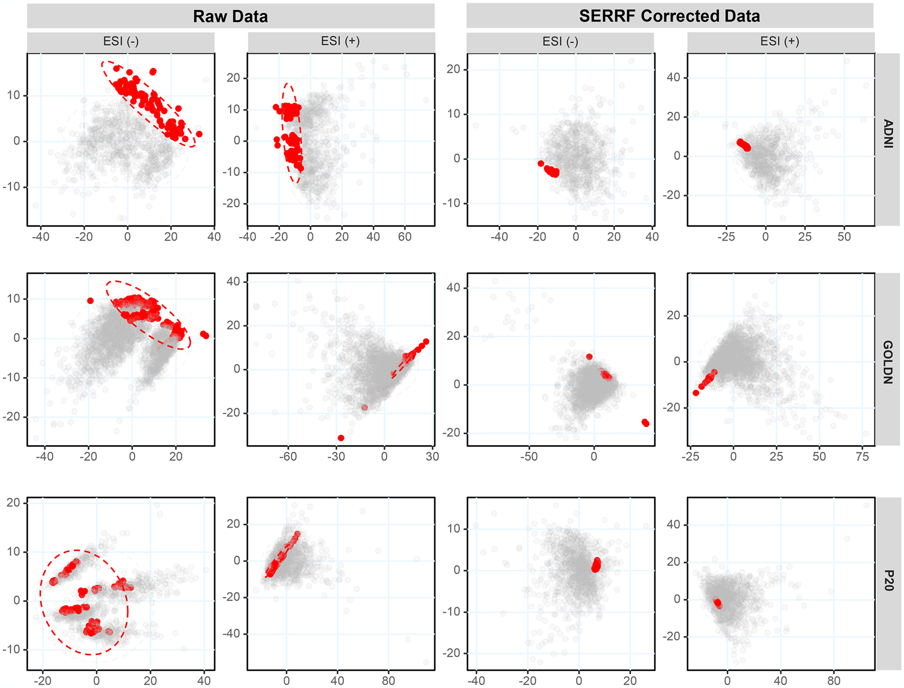
Principal component analysis score plots obtained before (left) and after (right) SERRF normalization for three human plasma lipidomics data sets acquired in (−) and (+) electrospray mode. QC samples are represented as red dots, while human cohort samples are black dots. The x-axes represent PC1, and y-axes are PC2.

We observed distinct clusters within and between data acquisition batches for QC samples in the raw data sets. Specifically, clusters were apparent in the PCA score plots for four data sets [all three ESI(−) cohort data and one ESI(+) data set] in addition to other unexplained variance for two other ESI(+) data sets (Figure 2, left). After SERRF normalization, all QC samples in the six data sets were aggregated to one tight cluster, with largely tightened QC distribution and no relationship to run orders or acquisition batches. This result indicates that batch effects and data drifts were effectively reduced by SERRF normalization.

Evaluating SERRF Performance for Univariate Lipids.

We further evaluated the performance of systematic error elimination in a univariate way, using the distribution of cross-validated relative standard deviations (cvRSD). RSDs are a commonly adopted criterion to assess the reproducibility of bioanalytical methods is the relative standard deviation (RSD) of QC samples.³⁶ The RSD for each lipid in the QC samples is calculated by dividing the sample standard deviation by the sample mean using eq 3:

$${\text{RSD}}_i={\text{SD}}_i/{\text{Avg}}_i$$ (3)

where SD_i and Avg_i are the standard deviation and the average of the QC intensity of the ith compound, respectively. Proposed thresholds in metabolomics range from 20% to 30% RSD, but may be flexible depending on the size of sample sets.³⁷ However, multivariate statistics, including machine learning tools, are prone to overfitting. Hence, a normalization method might perfectly correct intensity drifts on QC samples but could perform poorly when applied to human cohort samples.

To avoid this problem, instead of calculating the QC sample RSD for each compound directly, we calculated the fivefold Monte Carlo cross-validated QC RSD (cvRSD). The detailed cross-validation procedure is summarized as follows: (1) For each compound, randomly select 80% of QC samples as training QCs to build the normalization model. (2) Apply the model on the rest of the QC samples and calculate the RSD on these QC samples to validate the method. (3) Repeat 1 and 2 for five times with different sampling of model-building QC samples. (4) Calculate the mean average of the five validating QC RSDs as the cross-validated QC RSD to assess the performance of normalization on each compound. (5) Calculate the median of the cross-validated QC RSDs for all the compounds as the final performance measurement of the normalization method.

Because the validating QCs were not being used while training the models, we can use them to access the model performance with little risk of overfitting. An ideal sample normalization procedure should yield a low cvRSD. Here we compared SERRF with 15 commonly used normalization methods including nine data-driven normalization methods, two IS-based methods, and four QC-based normalization methods (Table S1).

SERRF-normalized data showed a consistent lower cvRSD (Table 2) and a large increase of the number of compounds with <20% of cvRSD compared to the raw data and batchwise LOESS-normalized data (Table 3). These results show that SERRF-normalized data sets become much more valid for subsequent univariate statistical analysis and biomarker discovery. When comparing SERRF to the 15 commonly used normalization methods for all six data sets, we observed that most normalization methods indeed achieved large improvements in cvRSD in comparison to the raw input data (Figure 3). We used Wilcoxon signed-rank tests to test the significance of performance improvement. SERRF was found to perform significantly better (p = 0.008) than the second-best method, batchwise LOESS normalization. Therefore, SERRF normalization significantly reduced systematic errors (in terms of cvRSD) compared to all other methods. We further confirmed that the improvement in cvRSD by SERRF was largely independent of the absolute signal intensity (Figure S1). SERRF almost uniformly outperformed all other methods across average lipid intensities. Last, we showed SERRF normalization yielded an average of 5% cvRSD across all six data sets and across all lipids, ranging from 3.4% to 7.3% cvRSD in all three cohort studies (Table 2). In comparison, batchwise LOESS normalization yielded a 2-fold higher residual error with an average of 9.8% cvRSD (ranging from 8.2% to 12.3% cvRSD) compared to SERRF. Raw data showed an average of 23.7% cvRSD across all six data sets, implying that the raw data acquisition was already at an acceptable quality but showed much improvement during data normalization.

Table 2.

Median Cross-Validated Relative Standard Deviations (cvRSD) in Three Lipidomic Human Cohorts

data set	raw data (%)	LOESS (%)	SERRF (%)
ADNI LC–ESI(−)-MS	23.2	12.3	7.3
ADNI LC–ESI(+)-MS	17.5	11.3	4.4
GOLDN LC–ESI(−)-MS	34.1	8.4	4.7
GOLDN LC–ESI(+)-MS	21.6	8.9	3.4
P20 LC–ESI(−)-MS	26.5	8.2	6.3
P20 LC–ESI(+)-MS	19.7	9.8	3.9

Table 3.

Percentage of Lipids with cvRSD < 20% in Three Lipidomic Human Cohorts

data set	raw data (%)	LOESS (%)	SERRF (%)
ADNI LC–ESI(−)-MS	31.9	84.6	88.7
ADNI LC–ESI(+)-MS	58.3	69.9	96.0
GOLDN LC–ESI(−)-MS	1.3	9.0	86.9
GOLDN LC–ESI(+)-MS	38.8	72.0	95.5
P20 LC–ESI(−)-MS	7.5	91.8	93.7
P20 LC–ESI(+)-MS	52.1.7	94.8	98.5

Figure 3.

Box-and-whisker plots of median cross-validated relative standard deviations (cvRSD) of the ESI(+) and ESI(−) lipidomic data sets for each normalization method.

Performance of Biomarker Selection and Classification Accuracy.

The aim of data normalization is to reveal true biological signals by removing systematic errors and to enable biomarker discovery³⁸ through feature selection.^39,40 Each study presented here investigated different biological questions which will be published elsewhere. To validate that SERRF indeed unmasks known true biological differences, we used the two P20 data sets to distinguish sex discriminants before and after batchwise LOESS and SERRF normalization. To evaluate the performance, we conducted (i) power analysis and (ii) modeling prediction accuracy.

Statistical power is a key aspect of the experimental study.⁴¹ By removing the systematic errors, a valid sample normalization procedure should be able to increase the statistical power of detecting compounds that are associated with the factor of study interests. We used the R package SSPA^42,43 to calculate the statistical power of detecting compounds that are associated with sex. Figure 4A shows that, after SERRF normalization, a higher power is achieved than by either batchwise LOESS normalization or by using raw data. When using the Mann–Whitney U test, the number of significant lipid differences between men and women increased by 10–20% from raw data to LOESS and SERRF normalization. More than half of all detected lipids were found to be significant between men and women, despite the huge variance in lipid abundances due to the range of differences in body mass index, levels of physical activity, age, or nutritional factors that is always present in large human cohort studies. Commonly, 80% power thresholds are used when designing human cohort studies. For distinguishing lipid profiles between the sexes, this threshold was achieved at 88 and 102 samples for raw data but was reduced to only 76 and 92 samples when using SERRF normalization for ESI(−) and ESI(+), respectively.

Figure 4.

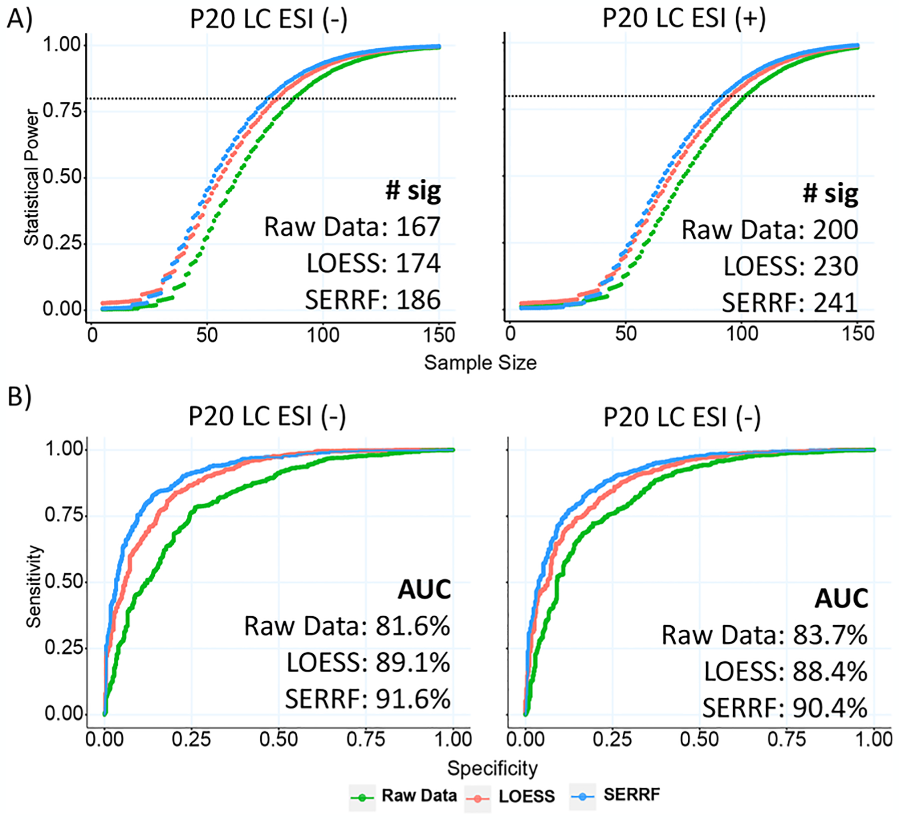
(A) Power analysis of the raw data, batchwise LOESS, and SERRF-normalized data set with the P20 study. SERRF achieved the highest statistical power. The bottom-right panel shows the number of significant compounds identified by the Mann–Whitney U test. More significant compounds were detected using the SERRF-normalized data set. (B) ROC of the GBM classifier using the raw data, batchwise LOESS, and SERRF-normalized data sets. Input variables are chosen based on a Mann–Whitney U test p-value <0.05 and PLS-DA VIP score >1. SERRF outperformed batchwise LOESS achieving the highest 5-fold cross-validated AUC (as shown at bottom-right).

The diagnostic ability of discriminating biomarkers is evaluated by classification accuracy, measured by receiver–operator characteristic curves (ROC). We selected a set of best-performing lipid biomarkers based on Mann–Whitney U test p < 0.05 and partial least-squares discriminant analysis with variable importance in projection (PLS-DA VIP) score >1, to distinguish factor gender using a supervised machine learning classifier, gradient boosting machine (GBM). These biomarkers were used in GBM with 5-fold cross-validated ROCs (Figure 4B). SERRF-normalized data sets achieved the highest diagnostic ability using the area under the ROC curves (AUC), indicating SERRF was most effective in removing unwanted systematic variations for biomarker-based classifications.

CONCLUSIONS

We developed a novel QC sample based data normalization algorithm, systematic error removal using random forest, SERRF. SERRF corrects batch effects and time-dependent drifts in large-scale plasma lipidomics human cohort studies, but it can also be used for other metabolomic platforms. The main advantage of SERRF over other commonly used normalization approaches is that it can effectively utilize information from all correlating compounds when normalizing each individual metabolite. When tested with six data sets from three large-scale cohort studies, SERRF has been demonstrated to significantly improve the reproducibility of peak abundance of QC samples and increase the statistical power of detected compounds associated with the phenotype of interest. We provide a free Web site-based (http://serrf.fiehnlab.ucdavis.edu) toolbox to implement SERRF to benefit the lipidomics and metabolomics community.

In this study, we used a ratio of cohort samples to QC samples of approximately 10:1. We have not tested how altering this ratio might influence the performance of the SERRF normalization. All six data sets used here included at least 800 cohort samples and 80 QC samples. Using SERRF for cohorts with fewer than 500 samples has not been tested. SERRF performance may vary or not be necessary for very small data sets.

REFERENCES

- (1).Keurentjes JJ; Fu J; De Vos CR; Lommen A; Hall RD; Bino RJ; van der Plas LH; Jansen RC; Vreugdenhil D; Koornneef M Nat. Genet 2006, 38 (7), 842. [DOI] [PubMed] [Google Scholar]
- (2).Fernie AR; Tohge T Annu. Rev. Genet 2017, 51, 287–310. [DOI] [PubMed] [Google Scholar]
- (3).Tzoulaki I; Ebbels TM; Valdes A; Elliott P; Ioannidis JP Am. J. Epidemiol 2014, 180 (2), 129–139. [DOI] [PubMed] [Google Scholar]
- (4).Zhang A; Sun H; Yan G; Wang P; Wang X BioMed Res. Int 2015, 2015, 354671. [DOI] [PMC free article] [PubMed] [Google Scholar]
- (5).Bijlsma S; Bobeldijk I; Verheij ER; Ramaker R; Kochhar S; Macdonald IA; Van Ommen B; Smilde AK Anal. Chem 2006, 78 (2), 567–574. [DOI] [PubMed] [Google Scholar]
- (6).Dunn WB; Wilson ID; Nicholls AW; Broadhurst D Bioanalysis 2012, 4 (18), 2249–2264. [DOI] [PubMed] [Google Scholar]
- (7).Martin J-C; Maillot M; Mazerolles G; Verdu A; Lyan B; Migne C; Defoort C; Canlet C; Junot C; Guillou C; et al. Metabolomics 2015, 11 (4), 807–821. [DOI] [PMC free article] [PubMed] [Google Scholar]
- (8).Sampson JN; Boca SM; Shu X-O; Stolzenberg-Solomon RZ; Matthews CE; Hsing AW; Tan Y-T; Ji B-T; Chow W-H; Cai Q; et al. Cancer Epidemiol., Biomarkers Prev 2013, 22, 631–640. [DOI] [PMC free article] [PubMed] [Google Scholar]
- (9).Li B; Tang J; Yang Q; Li S; Cui X; Li Y; Chen Y; Xue W; Li X; Zhu F Nucleic Acids Res. 2017, 45 (W1), W162–W170. [DOI] [PMC free article] [PubMed] [Google Scholar]
- (10).Zacharias H; Altenbuchinger M; Gronwald W Metabolites 2018, 8 (3), 47. [DOI] [PMC free article] [PubMed] [Google Scholar]
- (11).Chetwynd AJ; Abdul-Sada A; Holt SG; Hill EM Journal of Chromatography A 2016, 1431, 103–110. [DOI] [PubMed] [Google Scholar]
- (12).Borrego SL; Fahrmann J; Datta R; Stringari C; Grapov D; Zeller M; Chen Y; Wang P; Baldi P; Gratton E; Fiehn O; Kaiser P Cancer Metab. 2016, 4 (1), 9. [DOI] [PMC free article] [PubMed] [Google Scholar]
- (13).Sysi-Aho M; Katajamaa M; Yetukuri L; Orešič M BMC Bioinf. 2007, 8 (1), 93. [DOI] [PMC free article] [PubMed] [Google Scholar]
- (14).Redestig H; Fukushima A; Stenlund H; Moritz T; Arita M; Saito K; Kusano M Anal. Chem 2009, 81 (19), 7974–7980. [DOI] [PubMed] [Google Scholar]
- (15).Bromke MA; Sabir JS; Alfassi FA; Hajarah NH; Kabli SA; Al-Malki AL; Ashworth MP; Méret M; Jansen RK; Willmitzer L PLoS One 2015, 10 (10), e0138965. [DOI] [PMC free article] [PubMed] [Google Scholar]
- (16).Yang S; Sadilek M; Lidstrom ME Journal of chromatography A 2010, 1217 (47), 7401–7410. [DOI] [PMC free article] [PubMed] [Google Scholar]
- (17).Boysen AK; Heal KR; Carlson LT; Ingalls AE Anal. Chem 2018, 90 (2), 1363–1369. [DOI] [PubMed] [Google Scholar]
- (18).Livera AMD; Sysi-Aho M; Jacob L; Gagnon-Bartsch JA; Castillo S; Simpson JA; Speed TP Anal. Chem 2015, 87 (7), 3606–3615. [DOI] [PMC free article] [PubMed] [Google Scholar]
- (19).Wang S-Y; Kuo C-H; Tseng YJ Anal. Chem 2013, 85 (2), 1037–1046. [DOI] [PubMed] [Google Scholar]
- (20).Kamleh MA; Ebbels TM; Spagou K; Masson P; Want EJ Anal. Chem 2012, 84 (6), 2670–2677. [DOI] [PubMed] [Google Scholar]
- (21).Li B; Tang J; Yang Q; Cui X; Li S; Chen S; Cao Q; Xue W; Chen N; Zhu F Sci. Rep 2016, 6, 38881. [DOI] [PMC free article] [PubMed] [Google Scholar]
- (22).Cleveland WS; Devlin SJ J. Am. Stat. Assoc 1988, 83 (403), 596–610. [Google Scholar]
- (23).Luan H; Ji F; Chen Y; Cai Z Anal. Chim. Acta 2018, 1036, 66–72. [DOI] [PubMed] [Google Scholar]
- (24).Karpievitch YV; Nikolic SB; Wilson R; Sharman JE; Edwards LM PLoS One 2014, 9 (12), e116221. [DOI] [PMC free article] [PubMed] [Google Scholar]
- (25).Smolinska A; Blanchet L; Coulier L; Ampt KA; Luider T; Hintzen RQ; Wijmenga SS; Buydens LM PLoS One 2012, 7 (6), e38163. [DOI] [PMC free article] [PubMed] [Google Scholar]
- (26).Shah AD; Bartlett JW; Carpenter J; Nicholas O; Hemingway H Am. J. Epidemiol 2014, 179 (6), 764–774. [DOI] [PMC free article] [PubMed] [Google Scholar]
- (27).Rodriguez-Galiano VF; Ghimire B; Rogan J; Chica-Olmo M; Rigol-Sanchez JP ISPRS Journal of Photogrammetry and Remote Sensing 2012, 67, 93–104. [Google Scholar]
- (28).Díaz-Uriarte R; Alvarez de Andrés S BMC Bioinf. 2006, 7 (1), 3. [DOI] [PMC free article] [PubMed] [Google Scholar]
- (29).Barupal DK; Fan S; Wancewicz B; Cajka T; Sa M; Showalter MR; Baillie R; Tenenbaum JD; Louie G; Kaddurah-Daouk R; Fiehn O Sci. Data 2018, 5, 180263. [DOI] [PMC free article] [PubMed] [Google Scholar]
- (30).Cajka T; Fiehn O Methods Mol. Biol 2017, 1609, 149–170. [DOI] [PubMed] [Google Scholar]
- (31).Cajka T; Smilowitz JT; Fiehn O Anal. Chem 2017, 89 (22), 12360–12368. [DOI] [PubMed] [Google Scholar]
- (32).Cajka T; Davis R; Austin KJ; Newman JW; German JB; Fiehn O; Smilowitz JT Metabolomics 2016, 12 (8), 127. [Google Scholar]
- (33).Tu LN; Showalter MR; Cajka T; Fan S; Pillai VV; Fiehn O; Selvaraj V Sci. Rep 2017, 7 (1), 6120. [DOI] [PMC free article] [PubMed] [Google Scholar]
- (34).Breiman L Machine learning 2001, 45 (1), 5–32. [Google Scholar]
- (35).Touw WG; Bayjanov JR; Overmars L; Backus L; Boekhorst J; Wels M; van Hijum SA Briefings Bioinf. 2013, 14 (3), 315–326. [DOI] [PMC free article] [PubMed] [Google Scholar]
- (36).Parsons HM; Ekman DR; Collette TW; Viant MR Analyst 2009, 134 (3), 478–485. [DOI] [PubMed] [Google Scholar]
- (37).Kirwan JA; Weber RJ; Broadhurst DI; Viant MR Sci. Data 2014, 1, 140012. [DOI] [PMC free article] [PubMed] [Google Scholar]
- (38).Drabovich AP; Pavlou MP; Batruch I; Diamandis EP Proteomic AND Mass Spectrometry Technologies for Biomarker Discovery. In Proteomic and Metabolomic Approaches to Biomarker Discovery; Issaq HJ, Veenstra TD, Eds.; Elsevier: Amsterdam, The Netherlands, 2013; pp 17–37. [Google Scholar]
- (39).Liu H; Yu L IEEE Transactions on knowledge and data engineering 2005, 17 (4), 491–502. [Google Scholar]
- (40).García-Bilbao A; Armañanzas R; Ispizua Z; Calvo B; Alonso-Varona A; Inza I; Larrañaga P; López-Vivanco G; Suárez-Merino B; Betanzos M BMC Cancer 2012, 12 (1), 43. [DOI] [PMC free article] [PubMed] [Google Scholar]
- (41).Lipsey MW Design Sensitivity: Statistical Power for Experimental Research; Sage: Newbury Park, CA, 1990; Vol. 19. [Google Scholar]
- (42).Van Iterson M; t Hoen PAC; Pedotti P; Hooiveld G; Den Dunnen JT; van Ommen GJB; Boer JM; Menezes RX BMC Genomics 2009, 10 (1), 439. [DOI] [PMC free article] [PubMed] [Google Scholar]
- (43).Van Iterson M; van de Wiel MA; Boer JM; De Menezes RX Stat. Appl. Genet. Mol. Biol 2013, 12 (4), 449–467. [DOI] [PubMed] [Google Scholar]
Associated Data
This section collects any data citations, data availability statements, or supplementary materials included in this article.