Multi-Modal Imaging Genetics Data Fusion via a Hypergraph-Based Manifold Regularization: Application to Schizophrenia Study

Abstract

Recent studies show that multi-modal data fusion techniques combine information from diverse sources for comprehensive diagnosis and prognosis of complex brain disorder, often resulting in improved accuracy compared to single-modality approaches. However, many existing data fusion methods extract features from homogeneous networs, ignoring heterogeneous structural information among multiple modalities. To this end, we propose a Hypergraph-based Multi-modal data Fusion algorithm, namely HMF. Specifically, we first generate a hypergraph similarity matrix to represent the high-order relationships among subjects, and then enforce the regularization term based upon both the inter- and intra-modality relationships of the subjects. Finally, we apply HMF to integrate imaging and genetics datasets. Validation of the proposed method is performed on both synthetic data and real samples from schizophrenia study. Results show that our algorithm outperforms several competing methods, and reveals significant interactions among risk genes, environmental factors and abnormal brain regions.

I. Introduction

MULTI-MODAL data fusion has received enormous attention due to the rapid development of information acquisition from multiple sources. It provides richer information than a single modality by leveraging complementary information from multiple modalities, which is now widely used in various areas such as sensor networks, video processing, medical imaging and intelligent system design [1]–[5]. Multi-modal data are not only providing the high-dimensional features of traditional big data, but also are characterized by their diversity and heterogeneity. In the past few years, multi-modal data fusion studies were conducted to explore the shared feature representation and/or correlation between modalities [6], [7]. These data fusion methods are based on feature learning, but have not fully explored both the structure and cross-modality relationship among multi-modal data [8]. Thus, there has been a growing interest in fully mining the information of multi-modal data.

In the past decades, the sparse regularization methods, such as lasso, ridge and elastic net [9]–[11], were widely used in the feature selection. Following this, group lasso [12] and fused lasso [13] were developed as extensions of lasso to explore variables that are highly related. In other words, they incorporate prior knowledge by exploiting the network structure, which demonstrated improved performance in cancer marker discovery and disease phenotypes prediction [14], [15]. In addition, based on a weaker prior assumption, the truncated lasso penalty was applied for group variable selection [16]. Some techniques [17], [65]–[67] incorporated graphical structure to regularize sparse regression models. A manifold learning approach has been used to reduce the dimensionality of high-dimensional data [18], [68], [69], by learning high-dimensional correspondences from low-dimensional manifolds.

Furthermore, recent studies show that there is a common and specific information among different modalities, which can be incorporated into the integration of multiple imaging and genetics data for better understanding of disease mechanisms and improved diagnosis [19]–[27]. For example, Adeli et al. presented a multi-task multi-linear regression model for the prediction of multiple cognitive scores with incomplete longitudinal imaging data [19]. Jie et al. proposed a multi-task feature selection method based on hypergraphs for Alzheimer’s disease and mild cognitive impairment classification [20]. Zhu et al. proposed a multi-modal multi-task learning model to jointly select a small number of common features, followed by a support vector machine (SVM) to fuse these selected features for both classification and regression [21]. Du et al. proposed a novel multi-task SCCA (MTSCCA) method to identify bi-multivariate associations between single nucleotide polymorphism (SNP) data and multi-modal imaging quantitative traits [22]. Bai et al. applied a graph-based semi-supervised learning (GSSL) model to classify schizophrenia [23]. Based on deep learning network, an Auto-Encoder based Multi-View missing data Completion framework (AEMVC) was proposed [24] to learn common representations for AD diagnosis. Hu et al. developed an interpretable deep network-based multimodal fusion model to perform automated diagnosis and result interpretation simultaneously, which was further validated on a brain imaging-genetic study [25]. Most of these algorithms are based on networks to incorporate the relationships among multi-modal data. In addition, by examining the relationship of subjects in multiple modalities, significant co-occurrence information can be exploited [27].

However, imaging genetics data have high dimension but low sample size, and each modality of data has its own distribution due to its diversity. Most existing approaches reduced the dimension of each data separately and utilized similarity scores to find the links between modalities, and as a result overlooked the complex interactions among multi-modal data. In addition, many graph-based methods only capture the pairwise relationships, while ignoring higher order relationship among multiple data.

To overcome the above limitations, in this paper, we propose a novel multi-modal data fusion algorithm via the hypergraph-based manifold regularization, namely HMF, to integrate multiple imaging and genetics data types. Motivated by the work in [20], we extend the manifold regularized multitask learning model by replacing the manifold regularization term with the high-order relationship among subjects defined by a hypergraph. Furthermore, inspired by the multi-view spectral clustering incorporates all available information from multi-views to deliver the best clusters [33], we consider the similarity relationship of subjects both within and across modalities by enforcing a novel manifold regularization into our regression model. Specifically, the similarity of subjects between different modalities is calculated by propagating the similarity of subjects within individual modality. To validate our model, HMF is applied to both synthetic data and real samples from a dataset on schizophrenia (SZ) study collected by the MIND Clinical Imaging Consortium (MCIC) [28]. The simulation results show that the algorithm is robust and can extract more discriminative features from multi-modal data, resulting in higher classification accuracy than other competing algorithms. In particular, we show that integrating SNP, DNA methylation and functional magnetic resonance imaging (fMRI) data using our proposed algorithm led to better performance than using single type of data in terms of both SZ classification and biomarker detection.

There are five key contributions of this paper. First, complementary information is combined from multi-modal data by jointly learning common features, and our proposed algorithm results in better performance compared to several existing models. Second, a hypergraph-based similarity matrix is defined to better characterize high-order structural relationship between subjects than a simple graph representation. Third, we employ a novel manifold regularization term to incorporate the structural information both within and across modalities. Fourth, enforcing both sparsity and manifold regularization can incorporate both structural information and complex interactions among subjects, which can circumvent the overfitting problem in high dimension but low sample data. Fifth, we validated the proposed model on real schizophrenia data, and the experimental results demonstrated its. The model is easier to interpret than deep learning models, and we used it to identify the risk genes and abnormal brain ROIs involved in schizophrenia.

The remainder of this paper is organized as follows. Section II gives the notations of hypergraphs and introduces the proposed hypergraph-based multi-modal data fusion method. Section III presents the experimental results on the simulated data and the MCIC data with some discussions. Section IV concludes this paper.

II. Methods

As a multi-modal data fusion technique, joint feature learning extracts important features based on the similarity between multiple datasets. Suppose the datasets are obtained from K modalities, i.e., ${\mathbf{X}}^{(k)}={\left[{\mathit{x}}_1^{(k)},{\mathit{x}}_2^{(k)},\dots ,{\mathit{x}}_M^{(K)}\right]}^{\text{T}}$, ${\mathbf{X}}^{(k)}\in {ℝ}^{M\times d_k}(k=1,2,\dots ,K)$, where ${\mathit{x}}_m^{(k)}\in {ℝ}^{d_k}(m=1,2,\dots ,M)$ represents the features of the m-th sample from the k-th modality, M is the number of samples, and d_k denotes the number of features in the k-th modality. The response vector is denoted by y = [y₁, y₂, …, y_M ]^T, where y_m ∈ {−1, 1} is the class label of the m-th subject. Then the multimodal joint learning model is formulated to solve the following optimization problem:

$$\underset{{\mathbf{w}}^{(1)},{\mathbf{w}}^{(2)},\dots ,{\mathbf{w}}^{(K)}}{\min }\frac{1}{2}\sum _{k=1}^K\left[{‖\mathbf{y}-{\mathbf{X}}^{(k)}{\mathbf{w}}^{(k)}‖}_2^2+\lambda {‖{\mathbf{w}}^{(k)}‖}_1\right]$$ (1)

where w^(k) is the regression coefficient vector and λ is a regularization parameter that balances the tradeoff between fitting error and sparsity. The L₁-norm ensures that a sparse set of features can be learned from each modality.

A. Hypergraph-Based-Manifold Regularization

In the joint feature learning model, the observations of multi-modal data are utilized to fit the response, but the structure of the data is ignored. Considering that similar subjects should share the same labels or phenotypes, subject-subject relationships are therefore used as the regularization term to regularize the multi-modal joint learning model [27].

$${\sum }_{k=1}^K{S^{\prime }}_{ij}^{(k)}{\left({\widehat{y}}_i^{(k)}-{\widehat{y}}_j^{(k)}\right)}^2$$ (2)

where ${\widehat{y}}_i^{(k)}$ is the estimated response vector of the i -th subject in the k-th modality, and ${{\mathbf{S}}^{\prime }}^{\left(k\right)}=\left[{S^{\prime }}_{ij}^{(k)}\right]\in {ℝ}^{M\times M}$ is the symmetric similarity matrix denoting pairwise relationships in the k-th modality. However, in many practical problems, the relationship among subjects is more complex, involving three or more subjects. Such high-order relationships cannot be described by traditional graphs [29], [30]. Therefore, hypergraph learning has been [29], [63].

Unlike the edge in a traditional graph, the hyperedge in the hypergraph can connect more than two vertices. It is obvious that traditional graphs can be seen as a special example of hypergraphs. High-order relationships between vertices can be better captured by hypergraphs as shown in Fig. 1. A hypergraph $\mathbf{G}=(\mathbf{V},\mathbf{E},\mathit{\psi })$ is denoted by the vertex set $\mathbf{V}=\left\{v_1,v_2,\dots ,v_P\right\}$, the hyperedge set $\mathbf{E}=\left\{e_1,e_2,\dots ,e_Q\right\}$, and the hyperedge weight vector $\mathit{\text{ψ}}=\left[\psi \left(e_1\right),\psi \left(e_2\right),\dots ,\psi \left(e_Q\right)\right]$.

Fig. 1.

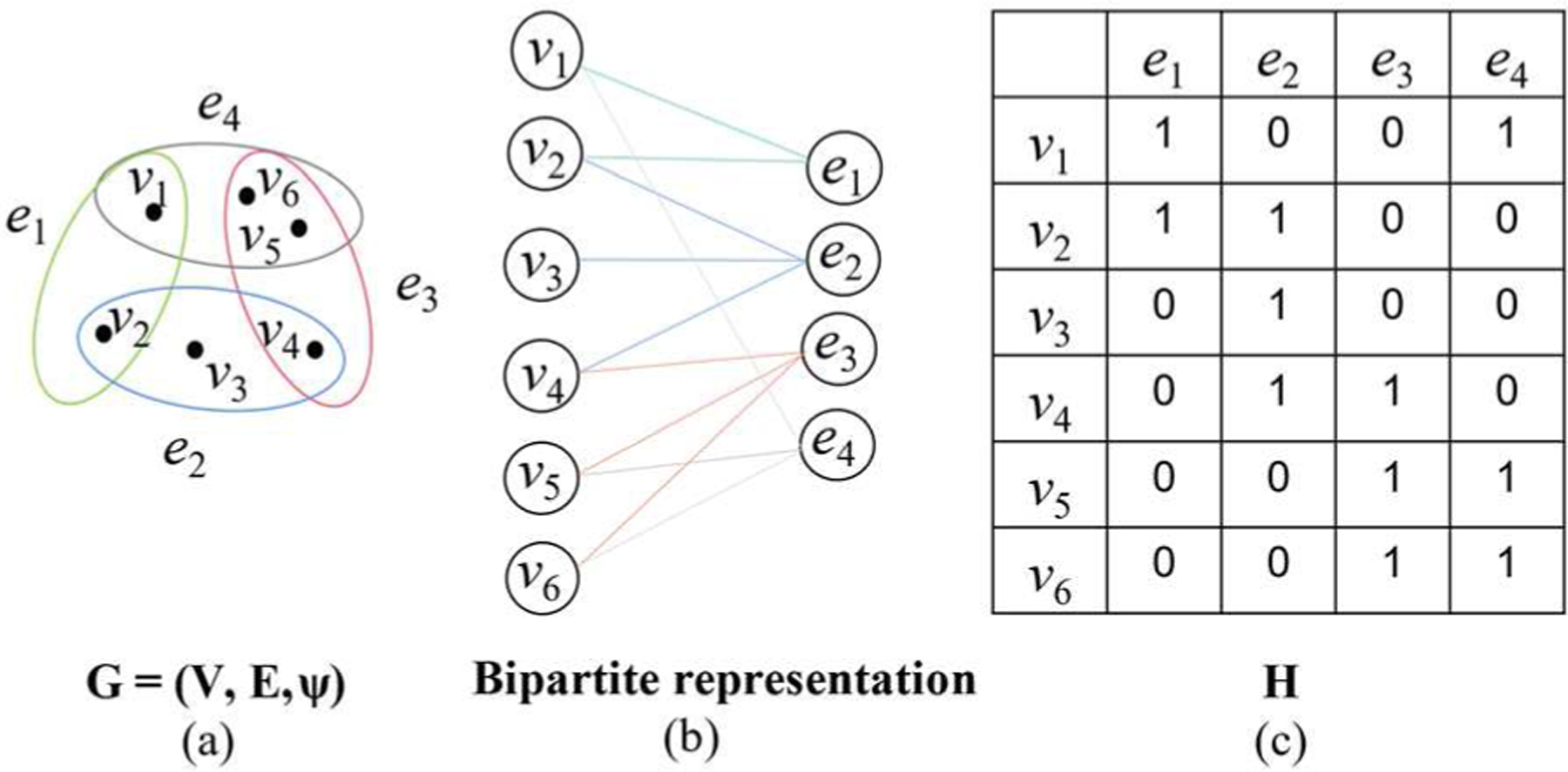
(a) A hypergraph G with vertex set V, hyperedge set E and hyperedge weight vector ψ. (b) Bipartite representation of hypergraph G. (c) The incidence matrix H of hypergraph G.

A hypergraph G can be represented by the incidence matrix $\mathbf{H}=\left[H_{pq}\right]\in {ℝ}^{P\times Q}$ with entries

$$H_{pq}=\left\{\begin{array}{ll}1,\hfill & if v_p\in e_q\hfill \\ 0,\hfill & \text{otherwise}\hfill \end{array}\right.$$ (3)

The vertex degree and hyperedge degree are defined respectively by

$$d\left(v_p\right)={\sum }_{e_q\in E}\psi \left(e_q\right)H_{pq}\text{\hspace{1em}for }1\le p\le P$$ (4)

$$\varphi \left(e_q\right)={\sum }_{v_p\in V}{H}_{pq}\text{\hspace{1em}for }1\le q\le Q$$ (5)

In addition, the diagonal matrices of the vertex degrees and the hyperedge degrees are denoted by ${\mathbf{D}}_{\mathit{v}}=\text{diag}\left(d\left(v_1\right),d\left(v_2\right),\dots ,d\left(v_P\right)\right)\in {ℝ}^{P\times P}$ and ${\mathbf{D}}_{\mathit{\text{e}}}=\text{diag}\left(\varphi \left(e_1\right),\varphi \left(e_2\right),\dots ,\varphi \left(e_Q\right)\right)\in {ℝ}^{Q\times Q}$, respectively. The diagonal matrix of the hyperedge weight is indicated by $\mathbf{\Psi }=\text{diag}\left(\psi \left(e_1\right),\psi \left(e_2\right),\dots ,\psi \left(e_Q\right)\right)\in {ℝ}^{Q\times Q}$. The similarity relationship between two vertices v_i and v _j in a hypergraph is represented by calculating the proportional weights over all hyperedges between v_i and v _j

$$S_{ij}={\sum }_{e_q\in E}\frac{\psi \left(e_q\right)}{\varphi \left(e_q\right)}{H}_{iq}{H}_{qj}$$ (6)

and the similarity matrix S of hypergraph G is defined by

$$\mathbf{S}=\mathbf{H}\mathbf{\Psi }{\mathbf{D}}_{\mathit{e}}^{-\mathbf{1}}{\mathbf{H}}^{\mathbf{T}}$$ (7)

where $\mathbf{S}=\left[S_{ij}\right]\in {ℝ}^{M\times M}$. Similar to the traditional graph Laplacian matrix, the hypergraph Laplacian matrix is denoted as $\mathbf{L}={\mathbf{D}}_{\mathit{\text{v}}}-\mathbf{S}$. Then, Eq. 2 can be rewritten in the hypergraph-based form

$$\frac{1}{2}\sum _{i,j=1}^M{S}_{ij}{\left({\widehat{y}}_i-{\widehat{y}}_j\right)}^2={\left(\widehat{\mathbf{y}}\right)}^{\text{T}}\mathbf{L}\left(\widehat{\mathbf{y}}\right)={\left(\mathbf{X}\mathbf{w}\right)}^{\text{T}}\mathbf{L}\left(\mathbf{X}\mathbf{w}\right)$$ (8)

In Eq. 7, the similarity matrix S is determined by the incidence matrix H and the hyperedge weight $\mathbf{\Psi }$. Here we employ the Ḱ-nearest neighbor strategy proposed in [31] to obtain the hypergraph. More specifically, by taking each vertex in a hypergraph as the center node, we calculate the Euclidean distance between the center node and other vertices. Then we connect each center node and its Ḱ nearest neighbor vertices to obtain the incidence matrix $\mathbf{H}\in {ℝ}^{M\times M}$. For M subjects, M hyperedges are constructed in total. In this paper, the hyperedge weight value ψ(e) is set to 1 based on the work [32].

B. Hypergraph-Based Multi-Modal Data Fusion

In order to preserve the basic structure and high-order information of data, an objective function is introduced by combining Eq. 1 and Eq. 8.

$$\begin{gathered} \underset{{\mathbf{w}}^{\left(1\right)},{\mathbf{w}}^{\left(2\right)},\dots ,{\mathbf{w}}^{\left(k\right)}}{\min }\frac{1}{2}\sum _{k=1}^K\left[{‖\mathbf{y}-{\mathbf{X}}^{\left(k\right)}{\mathbf{w}}^{\left(k\right)}‖}_2^2+{\lambda }_k{‖{\mathbf{w}}^{\left(k\right)}‖}_1\right] \\ +\mu \sum _{k=1}^K{\left({\mathbf{X}}^{(k)}{\mathbf{w}}^{(k)}\right)}^{\text{T}}{\mathbf{L}}^{(k)}\left({\mathbf{X}}^{(k)}{\mathbf{w}}^{(k)}\right) \end{gathered}$$ (9)

where λ_k and µ are two regularization parameters. However, only the high-order structure within each single homogeneous modality is considered in Eq. 9, while the relations across heterogeneous modalities (e.g., fMRI and SNPs) are ignored.

Motivated by this, we propose a novel hypergraph-based multi-modal data fusion algorithm incorporating both the relationships of subjects within a single modality and that between different modalities (as shown in Fig. 2). A new regularization term is then designed as

$$\text{Θ}\left(\mathbf{w},\alpha ,\beta \right)=\frac{1}{2}\sum _{a,b}^K\sum _{i,j}^M{\rho }^{\left(a,b\right)}{S}_{ij}^{\left(a,b\right)}{\left({\widehat{y}}_i^{\left(a\right)}-{\widehat{y}}_j^{\left(b\right)}\right)}^2$$ (10)

Fig. 2.

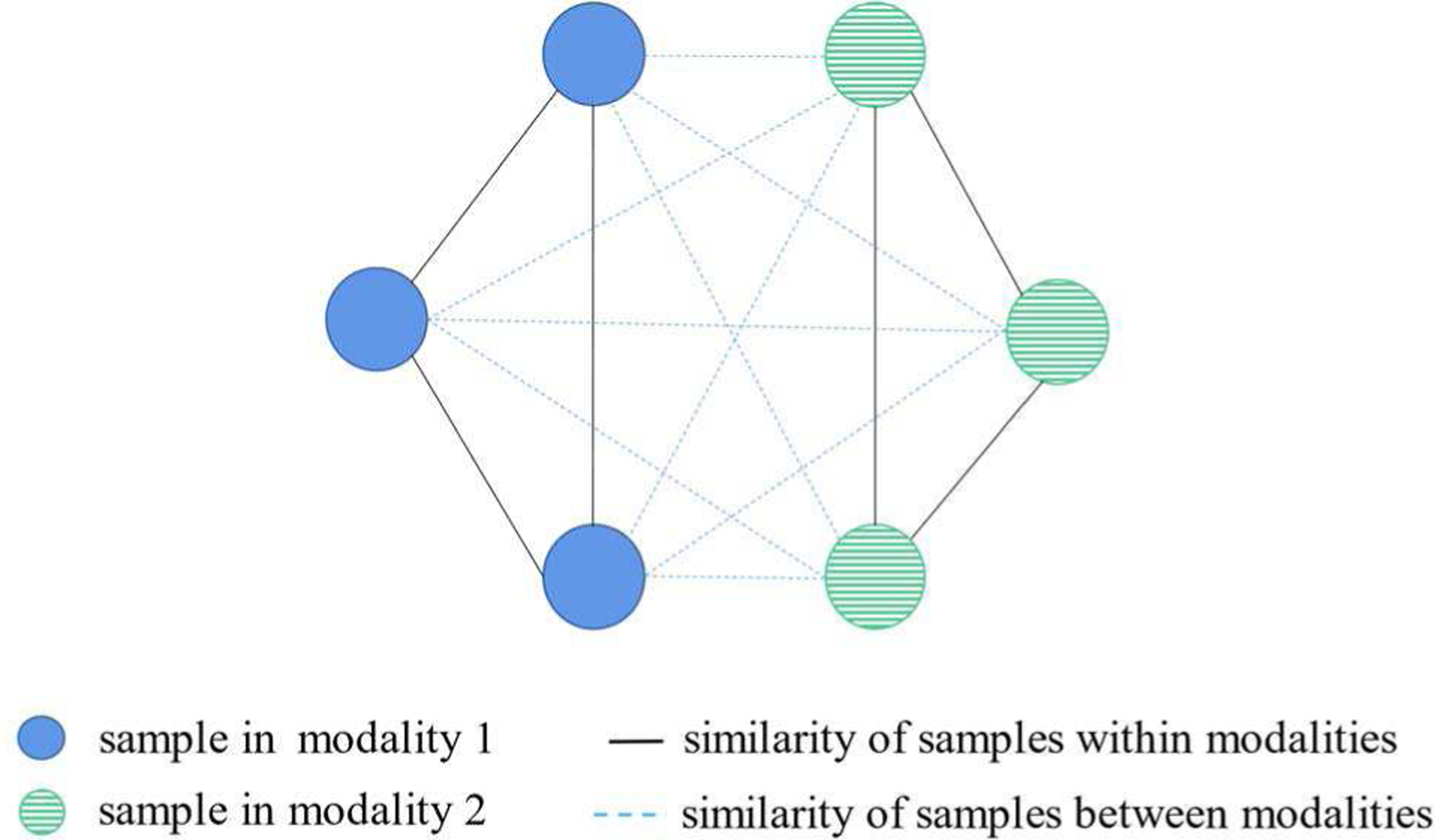
The illustration of the similarity relationship within and between different modalities.

It should be noted that the regularization term Θ(w, α, β) consists of two parts, ρ^(a,b) = α when a = b, and ρ^(a,b) = β when a ≠ b, corresponding to the constraints on a single modality and across modalities, respectively. The first part reads as

$$1/2\alpha {\sum }_a^K{\sum }_{i,j}^M{S}_{ij}^{(a)}{\left({\widehat{y}}_i^{(a)}-{\widehat{y}}_j^{(a)}\right)}^2$$ (11)

which calculates the high-order relationship of subjects within each single modality. The second part is

$$1/2\beta {\sum }_{a,b}^K{\sum }_{i,j}^M{S}_{ij}^{(a,b)}{\left({\widehat{y}}_i^{(a)}-{\widehat{y}}_j^{(b)}\right)}^2$$ (12)

which characterizes the inter-relationships of subjects between different modalities. α and β are two tuning parameters, and $y_i^{(a)}$ is the label of the i -th subject in the a-th modality. In Eq. 11, $S_{ij}^{(a)}$ denotes the hypergraph-based similarity of the i -th subject and the j -th subject with respect to the same modality, which can be calculated by Eq. 6. Likewise, in Eq. 12, $S_{ij}^{\left(a,b\right)}$ represents the similarity of the i -th subject in the a-th modality and the j -th subject in the b-th modality. We articulate that if two subjects ${\mathit{x}}_i^{(a)}$ and ${\mathit{x}}_j^{(a)}$ for the same modality are similar, the observation of subject x_i in another modality, e.g., ${\mathit{x}}_i^{\left(b\right)}$, should also be similar to ${\mathit{x}}_j^{(a)}$. According to previous work [33], [34], $S_{ij}^{\left(a,b\right)}$ measures the co-occurrence between the i -th subject and the j -th subject and between a and b modality among M subjects simultaneously, i.e.,

$$S_{ij}^{(a,b)}={\sum }_{m=1}^M{S}_{im}^{(a)}{S}_{mj}^{(b)}$$ (13)

The matrix form is ${\mathbf{S}}^{\left(a,b\right)}={\mathbf{S}}^{\left(a\right)}{\mathbf{S}}^{\left(b\right)}$, where ${\mathbf{S}}^{\left(a\right)}$ and ${\mathbf{S}}^{\left(b\right)}$ are the high-order similarity matrices for the a-th and b-th modalities and can be calculated by Eq. 7. A block-wise similarity matrix $\tilde{\mathbf{S}}\in {ℝ}^{MK\times MK}$ for all samples and modalities is denoted by

$$\tilde{\mathbf{S}}=\left[\begin{array}{ccc}{\mathbf{S}}^{(1,1)}& \cdots & {\mathbf{S}}^{(1,K)}\\ ⋮& \ddots & ⋮\\ {\mathbf{S}}^{(K,1)}& \cdots & {\mathbf{S}}^{(K,K)}\end{array}\right]$$ (14)

Then, the hypergraph Laplacian matrix can be calculated by $\tilde{\mathbf{L}}=\tilde{\mathbf{D}}-\tilde{\mathbf{S}}$. Since $\tilde{\mathbf{S}}$ is symmetrical, ${\tilde{\mathbf{D}}}_{ii}={\sum }_j{\tilde{\mathbf{S}}}_{ij}\text{ for }1\le i\le MK$. Considering the regularization parameters α and β, the block-wise form of matrix $\tilde{\mathbf{L}}$ is denoted as

$$\tilde{\mathbf{L}}=\left[\begin{array}{ccc}\alpha {\mathbf{L}}^{(1,1)}& \cdots & \beta {\mathbf{L}}^{(1,K)}\\ ⋮& \ddots & ⋮\\ \beta {\mathbf{L}}^{(K,1)}& \cdots & \alpha {\mathbf{L}}^{(K,K)}\end{array}\right]$$ (15)

In this way, Eq. 10 can be equivalently expressed as

$$\text{Θ}\left(\mathbf{w},\alpha ,\beta \right)={\left[\begin{array}{c}{\mathbf{X}}^{\left(1\right)}{\mathbf{w}}^{\left(1\right)}\\ {\mathbf{X}}^{\left(2\right)}{\mathbf{w}}^{\left(2\right)}\\ ⋮\\ {\mathbf{X}}^{\left(K\right)}{\mathbf{w}}^{\left(K\right)}\end{array}\right]}^{\text{T}}\tilde{\mathbf{L}}\left[\begin{array}{c}{\mathbf{X}}^{\left(1\right)}{\mathbf{w}}^{\left(1\right)}\\ {\mathbf{X}}^{\left(2\right)}{\mathbf{w}}^{\left(2\right)}\\ ⋮\\ {\mathbf{X}}^{\left(K\right)}{\mathbf{w}}^{\left(K\right)}\end{array}\right]$$ (16)

Using this regularization term expressed in Eq. 16, we propose the HMF model as follows

$$\begin{gathered} ℒ=\underset{{\mathbf{w}}^{(1)},{\mathbf{w}}^{(2)},\dots ,{\mathbf{w}}^{(k)}}{\min }1/2\sum _{k=1}^K\left[{‖\mathbf{y}-{\mathbf{X}}^{(k)}{\mathbf{w}}^{(k)}‖}_2^2+{\lambda }_k{‖{\mathbf{w}}^{(k)}‖}_1\right] \\ +\text{Θ}(\mathbf{w},\alpha ,\beta ) \end{gathered}$$ (17)

where α and β denote the parameters of hypergraph-based manifold regularization term that are used to tune the similarity of subjects both within the same modality and between different modalities (in Eq. 16). Fig. 3 illustrates the procedure of our approach based on this algorithm.

Fig. 3.

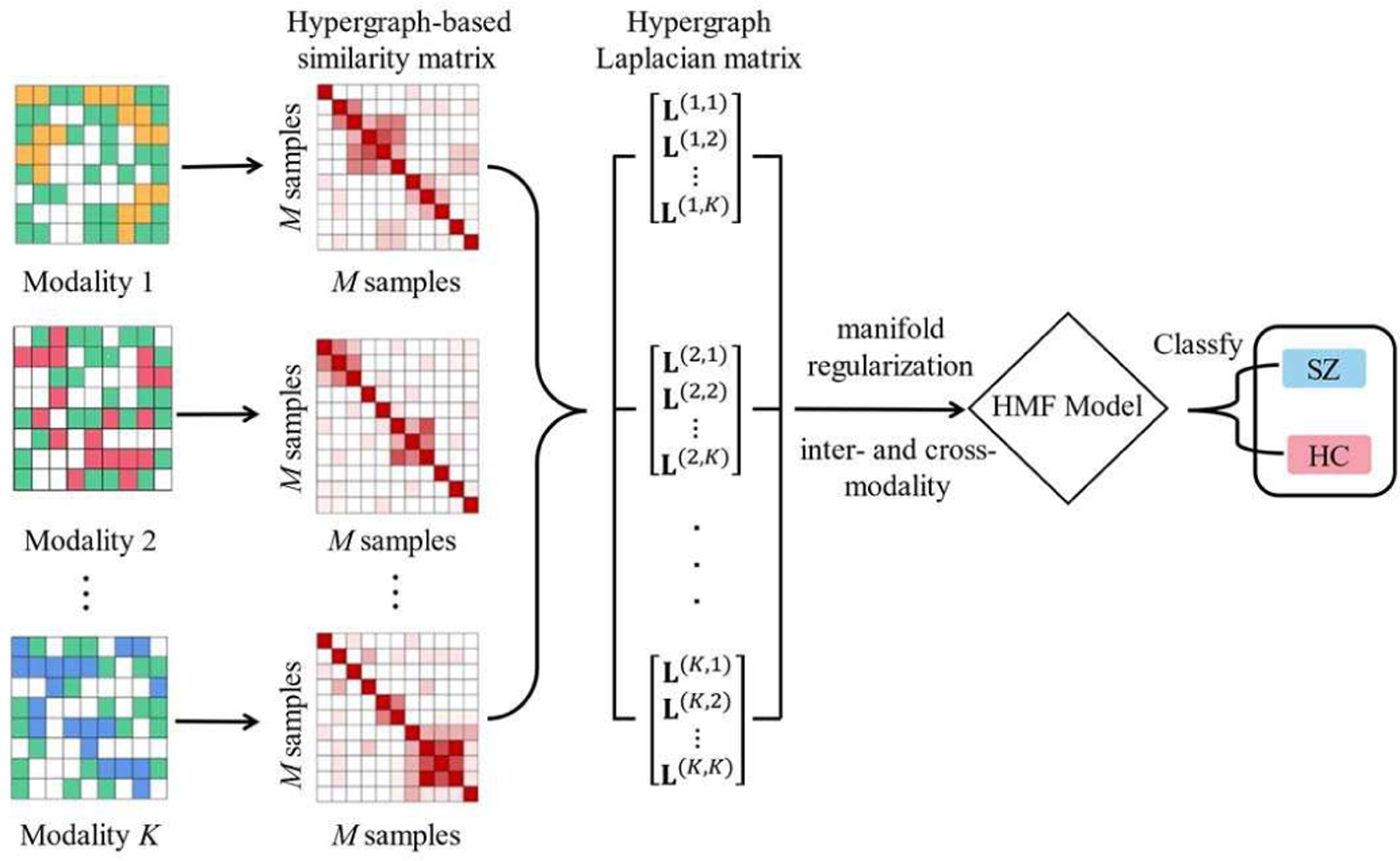
The main framework of the proposed algorithm.

C. Optimization

It is obvious that the object function in Eq. 17 is convex. To optimize w, we take the derivative of Eq. 17 with respect to w^(k),

$$\begin{gathered} \nabla ℒ\left({\mathbf{w}}^{(k)}\right)={\left({\mathbf{X}}^{(k)}\right)}^{\text{T}}\left({\mathbf{X}}^{(k)}{\mathbf{w}}^{(k)}-\mathbf{y}\right)+\alpha \sum _{k=1}^K{\left({\mathbf{X}}^{(k)}\right)}^{\text{T}}{\mathbf{L}}^{(k,k)} \\ \begin{array}{l}\times {\mathbf{w}}^{(k)}+\beta \sum _{a=1}^K\sum _{b=1}^K\left({\left({\mathbf{X}}^{(k)}\right)}^{\text{T}}{\mathbf{L}}^{(a,b)}{\mathbf{X}}^{(a)}{\mathbf{w}}^{(a)}\right)\\ +{\lambda }_k\mathrm{sgn}\left({\mathbf{w}}^{(k)}\right)(a\ne b,a\parallel b=k)\end{array} \end{gathered}$$ (18)

where sgn(·) is the signum function. Then the vector w^(k) can be iteratively updated as follows:

$$\begin{array}{l}{\mathbf{w}}^{(k)}\left(t+1\right)\\ ={\left({\left({\mathbf{X}}^{(k)}\right)}^{\text{T}}{\mathbf{X}}^{(k)}+\alpha {\left({\mathbf{X}}^{(k)}\right)}^{\text{T}}{\mathbf{L}}^{(k,k)}{\mathbf{X}}^{(k)}\right)}^{-1}\\ \times \left({\left({\mathbf{X}}^{(k)}\right)}^{\text{T}}\mathbf{y}-\beta \sum _{a=1}^K\sum _{b=1}^K\left({\left({\mathbf{X}}^{(k)}\right)}^{\text{T}}{\mathbf{L}}^{(a,b)}{\mathbf{X}}^{(a)}{\mathbf{w}}^{(a)}(t)\right)\right)\\ +{\lambda }_{k}sgn\left({\mathbf{w}}^{(k)}(t)\right)(a\ne b,a\parallel b=k)\end{array}$$ (19)

where t represents the t-th iteration. The iteration will terminate when the relative error of the objective function satisfies $\left|ℒ(t+1)-ℒ(t)\right|/\left|ℒ\left(t+1\right)\right|\le \epsilon \left(\epsilon ={10}^{-6}\right)$. The pseudocode of HMF is summarized in Algorithm 1.

$$\begin{array}{l}\overline{\underset{¯}{\begin{array}{l}\mathbf{Algorithm}\mathbf{1}\text{ The Hypergraph-Based\hspace{0.17em}Multi-Modal Data Fusion }\\ \text{(HMF)}\end{array}}}\\ \mathbf{Input}:K\text{\hspace{0.17em}modalities\hspace{0.17em}data\hspace{0.17em}}{\mathbf{X}}^{(k)},\text{label\hspace{0.17em}}\mathbf{y},\text{hyperparameters\hspace{0.17em}}\alpha ,\beta \text{\hspace{0.17em}and\hspace{0.17em}}{\lambda }_k(k=\\ 1,2,\dots ,K).\\ \mathbf{Output}\text{: weight vectors }{\mathbf{w}}^{(k)}(k=1,2,\dots ,K)\text{.}\\ \text{\hspace{0.33em}1: }\mathbf{Initialization}\text{: }{\mathbf{w}}^{(k)}(k=1,2,\dots ,K)\text{;}\\ \text{\hspace{0.33em}2: }\mathbf{for}k=1\text{ to }K\mathbf{do}\\ 3:\text{\hspace{1em}\hspace{1em}obtain\hspace{0.17em}}\mathbf{H}\text{\hspace{0.17em}and\hspace{0.17em}}\mathbf{w}\text{\hspace{0.17em}for\hspace{0.17em}each\hspace{0.17em}dataset}\\ \text{\hspace{0.33em}4:\hspace{1em}\hspace{1em}calculate }{\mathbf{S}}^{(k)}\text{ by Eq. }7\\ \text{\hspace{0.33em}5: }\mathbf{end}\mathbf{for}\\ \text{\hspace{0.33em}6: use }{\mathbf{S}}^{(k)}(k=1,2,\dots ,K)\text{ to get }\tilde{\mathbf{S}}\text{ and then calculate }\tilde{\mathbf{L}}\text{. }\\ 7\text{ : }\mathbf{for}t=1\text{ to }Max-Iteration\mathbf{do}\\ 8:\text{\hspace{1em}\hspace{1em}fix\hspace{0.33em}}{\mathbf{w}}^{(1)},\dots ,{\mathbf{w}}^{(k-1)},{\mathbf{w}}^{(k+1)}\dots ,{\mathbf{w}}^{(K)}\text{\hspace{0.33em}and\hspace{0.33em}update\hspace{0.33em}}{\mathbf{w}}^{(k)}\\ \text{\hspace{0.33em}\hspace{1em}\hspace{1em}\hspace{1em}by\hspace{0.33em}Eq.\hspace{0.33em}\hspace{0.33em}}19\\ \text{\hspace{0.33em}9: }\mathbf{until}\text{ converge }\\ 10:\mathbf{end}\mathbf{for}\\ \underset{¯}{11:\mathbf{Return}{\mathbf{w}}^{(k)}(k=1,2,\dots ,K).}\end{array}$$

III. Experimental Results and Analysis

A. The Simulated Data Experiment

1). Simulation Setup:

To evaluate the performance of the proposed algorithm, we first simulated three datasets with different properties and let the number of samples be smaller than the number of features to simulate high dimensionality of the data: ${\mathbf{X}}^{(1)}\in {ℝ}^{C\times d_1}$, ${\mathbf{X}}^{(2)}\in {ℝ}^{C\times d_2}$ and ${\mathbf{X}}^{(3)}\in {ℝ}^{C\times d_3}$, where C = 200 is the sample size, d₁ = 3000, d₂ = 4000 and d₃ = 5000 are the dimensions of features in three datasets, respectively. The simulation procedure is similar to the work in [35] with the following steps. First, four independent latent variables $z_1,z_2,z_3,z_4\in {ℝ}^{200\times 1}$ are generated following a standard multivariate normal distribution. Then three sparse vectors are created $\eta \in {ℝ}^{1\times d_i}$ and each dataset can be formed as:

$$\begin{gathered} {\mathbf{X}}^{(1)}=z_1{\text{η}}_1+z_2{\text{η}}_2+z_4{\text{η}}_3+{\mathbf{E}}_1 \\ {\mathbf{X}}^{(2)}=z_1{\text{η}}_4+z_3{\text{η}}_5+z_4{\text{η}}_6+{\mathbf{E}}_2 \\ {\mathbf{X}}^{(3)}=z_2{\text{η}}_7+z_3{\text{η}}_8+z_4{\text{η}}_9+{\mathbf{E}}_3 \end{gathered}$$ (20)

where each vector η contains 100 non-zero entries, and each of them follows a uniform distribution η_non−zeros ∼ U(0.4, 0.6). Here, the first 100 features of η₃, η₆ and η₉, the second 100 features of η₁ and η₄, the third 100 features of η₂ and η₇, and the fourth 100 features of η₅ and η₈ are all non-zeros, respectively. In this way, X⁽¹⁾ and X⁽²⁾ have 100 correlated features generated by latent variable z₁. X⁽¹⁾ and X⁽³⁾ have 100 correlated features generated by latent variable z₂. X⁽²⁾ and X⁽³⁾ have 100 correlated features generated by latent variable z₃. X⁽¹⁾, X⁽²⁾ and X⁽³⁾ have 100 correlated features generated by latent variable z₄. In addition, continuous labels are generated from these explanatory variables and then transformed to z-scores. The subjects whose scores are at the top and bottom 30% are selected from both ends, and M = 120 subjects are retained and labelled with binary number based on the scores. Finally, the noise signals ${\mathbf{E}}_1\in {ℝ}^{120\times 3000}$, ${\mathbf{E}}_2\in {ℝ}^{120\times 4000}$ and ${\mathbf{E}}_3\in {ℝ}^{120\times 5000}$ are added to three datasets to test the robustness of the algorithm and each noise signal follows a standard normal distribution.

2). Parameter Selection:

In the experiment, we used a 10-fold cross validation (CV) to assess the classification accuracy of all predictive models. That is, the dataset was first randomly divided into 10 disjoint subsets, and then each subset was selected as the test set, while the rest 9 subsets were used for training. This process was repeated 10 times, reducing the impact of sampling bias.

All regularization parameters in the models, including manifold regularization parameters α, β, the sparsity level λ₁, λ₂, λ₃, and the nearest neighbor size Ḱ were tuned through grid search within their respective ranges. Here we divided the parameter tuning process into three parts to reduce the excessive experiments. Fig. 4(a) displays the parameter tuning without sparsity constraint, i.e., α ∈ {10⁻², 2 × 10⁻², 3 × 10⁻², …, 10⁻¹}, β ∈ {10⁻³,2 × 10⁻³,3 × 10⁻³, …, 10⁻²}, Ḱ=9, λ₁, λ₂ and λ₃ = 0. Fig. 4(c) shows the selection of sparse parameters in their respective ranges λ₁, λ₂ ∈ {10⁻⁴, 2 × 10⁻⁴, …, 6 × 10⁻⁴} and λ₃ ∈ {3 × 10⁻⁴, 4 × 10⁻⁴, …, 8 × 10⁻⁴}, when α = 0.04, β = 0.006 and Ḱ=9. The parameter Ḱ for the hypergraph-based similarity matrix calculation was empirically set to 10 in [32]. As shown in Fig. 4(b), we optimized Ḱ in the range of {7, 8, …, 12}, and found that 9 worked relatively best in our experiments. Here, all parameters were tuned by a 10-fold inner CV on the training set and our model was sensitive within only a small range. According to their impact on classification, we finally set parameters as α = 0.04, β = 0.006, λ₁ = 0.0002, λ₂ = 0.0004, λ₃ = 0.0005 and Ḱ=9, which deliver the highest classification accuracy 91.80%.

Fig. 4.

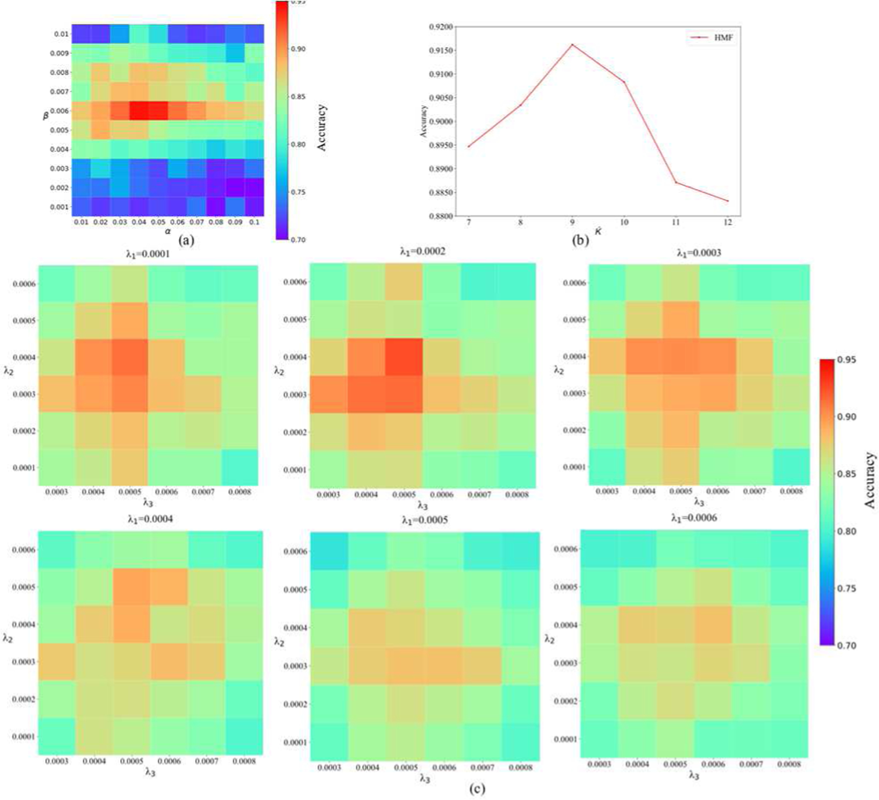
The classification performance of the proposed algorithm with respect to different parameters’ settings. (a) α ∈ {10⁻², 2 × 10⁻², 3 × 10⁻², …, 10⁻¹}, β ∈ {10⁻³, 2 × 10⁻³, 3 × 10⁻³, …, 10⁻²}, λ₁, λ₂, λ₃ = 0 and Ḱ = 9. (b) α = 0.04, β = 0.006, λ₁ = 0.0002, λ₂ = 0.0004, λ₃ = 0.0005 and Ḱ ∈ {7, 8, …, 12}. (c) α = 0.04, β = 0.006, Ḱ = 9, λ₁, λ₂ ∈ {10⁻⁴, 2 × 10⁻⁴, …, 6 × 10⁻⁴} and λ₃ ∈ {3 × 10⁻⁴, 4 × 10⁻⁴, …, 8 × 10⁻⁴}. (c) α = 0.04, β = 0.006, λ₁ = 0.0002, λ₂ = 0.0004, λ₃ = 0.0005 and Ḱ ∈ {7, 8, …, 12}.

3). Experiment Result on the Simulated Dataset:

In the experiments, we tested the proposed HMF algorithm on single-view data, pairwise combination and the combination of three types of data. We compared the performance of our model and five other models, e.g., Multi-task learning (MTL) [36], Similarity-network-fusion-based SVM (SNF-SVM) [37], majority neighborhood-based classification by mean fusion (MMN) [38], the graph-based semi-supervised learning (GSSL) [23], Grad-CAM guided convolutional collaborative learning (gCAM-CCL) [25], and manifold regularization multi-modal data fusion (MRMF) based on graph networks. Fig. 5(a) shows the performance of all compared algorithms. Specifically, our proposed HMF achieved the best classification accuracy 0.9250 ± 0.0293 (mean ± std) by integrating three datasets, which outperformed all the other methods, e.g., 0.9075 ± 0.0186 by MRMF, 0.7896 ± 0.0272 by gCAM-CCL, 0.8833 ± 0.0172 by GSSL, 0.7583 ± 0.0295 by MMN, 0.6833 ± 0.0249 by SNF-SVM and 0.5667 ± 0.0267 by MTL.

Fig. 5.

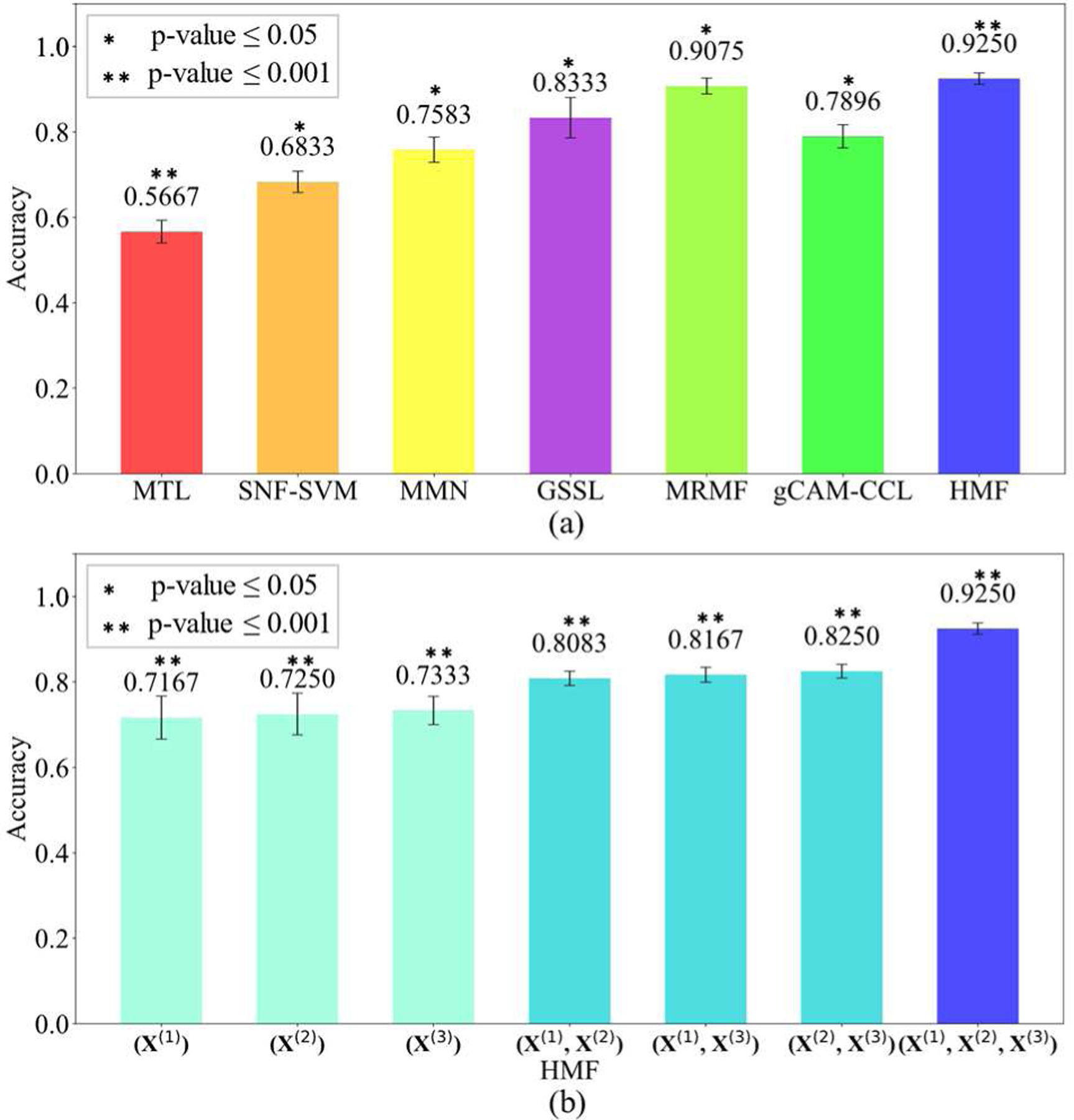
(a) The comparison of classification accuracies by HMF and 6 other algorithms. (b) The classification accuracies of HMF tested on different combinations of datasets.

In addition, we tested HMF when combining different datasets. As shown in Fig. 5(b), the classification accuracies of HMF on single dataset were 0.6833 ± 0.0137 for X⁽¹⁾, 0.6917 ± 0.0154 for X⁽²⁾ and 0.7167 ± 0.0163 for X⁽³⁾, which were lower than the accuracy of using pairwise combination, i.e., 0.8083 ± 0.0133 for X⁽¹⁾ and X⁽²⁾, 0.8167 ± 0.0129 for X⁽¹⁾ and X⁽³⁾, and 0.8250 ± 0.0128 for X⁽²⁾ and X⁽³⁾, respectively.

To further validate the algorithm, we also compared HMF and with other algorithms on the simulated data with different noise levels, i.e., signal-to-noise ratio (SNR), SNR ∈ [0.2, 0.4, 0.6, 0.8, 1.0]. Fig. 6(a) displays the error rates of HMF testing on the datasets added with 5 different SNRs. It can be found that integrating three views of data achieves least error rates than using a single or two datasets. In addition, we compared HMF with 6 other algorithms by testing the datasets added with 5 different SNRs. Fig. 6(b) displays that HMF obtains the lowest error rates in all 5 datasets.

Fig. 6.

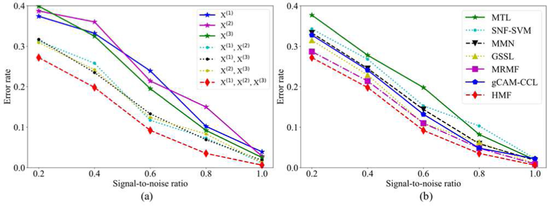
(a) The error rates of HMF when testing with the combination of different datasets and added with 5 different SNRs. (b) The error rates of 7 algorithms when testing on three−view datasets with 5 different SNRs.

B. Application to Classify Schizophrenia

1). Real Data Preparation and Preprocessing:

In the real data experiment, we tested our algorithm on clinical samples from schizophrenia study, which had SNP, DNA methylation and fMRI collected by the Mind Clinical Imaging Consortium (MCIC) [28]. The MCIC dataset contained 183 subjects, including 79 SZ patients (age: 34 ± 11, 20 females) and 104 healthy controls (age: 32 ± 11, 38 females).

The fMRI data were collected while subjects were performing a sensory motor task, a block design motor response to auditory stimulation. Standard pre-possessing steps were applied using SPM12, including motion correction, spatial normalization and resliced to 3 × 3 × 3 mm, spatial smoothing with a 10 × 10 × 10 mm³ Gaussian kernel. Then multiple regression considering the influence of motion was performed and the stimulus on-off contrast maps for each subject were collected [39]. As a result, a 53 × 63 × 46 stimulus-on versus stimulus-off contrast image was extracted for each participant. After excluding voxels with missing measurements, each image consists of 41, 236 voxels in total, which were divided into 116 ROIs based on the Automated Anatomical Labeling (AAL) template.

The SNPs data were obtained from blood samples of each subject. Genotyping was performed at the Mind Research Network, covering 1, 140, 419 SNP loci, out of which 722, 177 SNP loci were retained after quality control using PLINK package 3. Each SNP was categorized into three clusters based on their genotype and was represented by discrete numbers: 0 for ‘BB’ (no minor allele), 1 for ‘AB’ (one minor allele) and 2 for ‘AA’ (two minor alleles).

The DNA methylation data were also extracted from blood samples, which were assessed by the Illumina Infinium Methylation 27 k Assay. After excluding intensity outliers, the data were normalized by using the R package watermelon [40], which contained 27, 508 CpG loci. Each entry was between 0 and 1, representing the methylation level of each CpG island. More details about data collection and preprocessing can be found in the work [41], [42].

2). Experimental Results on Real Dataset:

To further validate the performance of our model, we tested our algorithm on the MCIC dataset and compared with other competing models, i.e., MTL, SNF-SVM, MMN, gCAM-CCL, MRMF and GSSL. A 10-fold cross-validation was applied to evaluate the classification performance for all these methods and ran 10 times independently on the whole 183 subjects. The model performance was quantified with both the classification accuracy and the root mean square error (RMSE) between predicted and true labels of the subjects in the testing set. The parameters of HMF were tuned in their respect ranges, i.e., α ∈ {10⁻², 2 × 10⁻², …, 10⁻¹}, β ∈ {10⁻³, 2 × 10⁻³, …, 10⁻²}, λ₁ ∈ {10⁻⁶, 2 × 10⁻⁶, …, 10⁻⁵}, λ₂, λ₃ ∈ {10⁻⁵, 2 × 10⁻⁵, …, 10⁻⁴} and Ḱ ∈ {5, 6, …, 10}, and finally set as α = 0.03, β = 0.006, λ₁ = 5 × 10⁻⁶, λ₂ = 3 × 10⁻⁵, λ₃ = ×10⁻⁵ and Ḱ=7, respectively.

Table I summarizes the performance of 7 algorithms when testing on the MCIC dataset. HMF achieves the best classification performance in both accuracy 0.8749 ± 0.0164 and RMSE 0.6902 ± 0.1053. MRMF, which can be regarded as the graph version of HMF, obtains the second-best accuracy 0.8479 ± 0.0162 and RMSE 0.7342 ± 0.0126. GSSL gets the accuracy 0.8202 ± 0.0217 and RMSE 0.7884 ± 0.1573, which are better than other models, e.g., accuracy 0.7721 ± 0.0224 and RMSE 0.7945 ± 0.1184 by gCAM-CCL, accuracy 0.6942 ± 0.0363 and RMSE 0.8646 ± 0.1749 by MMN, accuracy 0.5783 ± 0.0301 and RMSE 0.9331 ± 0.1937 by SNF-SVM, and accuracy 0.5470 ± 0.0339 and RMSE 1.3072 ± 0.2123 by MTL. The experimental results using the MCIC data demonstrate that the HMF with hypergraph-based manifold regularization indeed improves the accuracy while reduces RMSE by incorporating high-order structural information of subjects across modalities. We drew the ROC curves of all the compared algorithms testing on the MCIC dataset. As shown in Fig. 7, HMF achieves the best AUC = 0.91 (Area Under the Curve), which is higher than the graph networks-based model MRMF (AUC = 0.87) and the graph learning-based model GSSL (AUC = 0.84). Moreover, the performance of three manifold learning-based models are superior than that of other algorithms, i.e., AUC = 0.73 for gCAM-CCL, AUC = 0.63 for MMN, AUC = 0.58 for SNF-SVM and AUC = 0.43 for MTL.

Fig. 7.

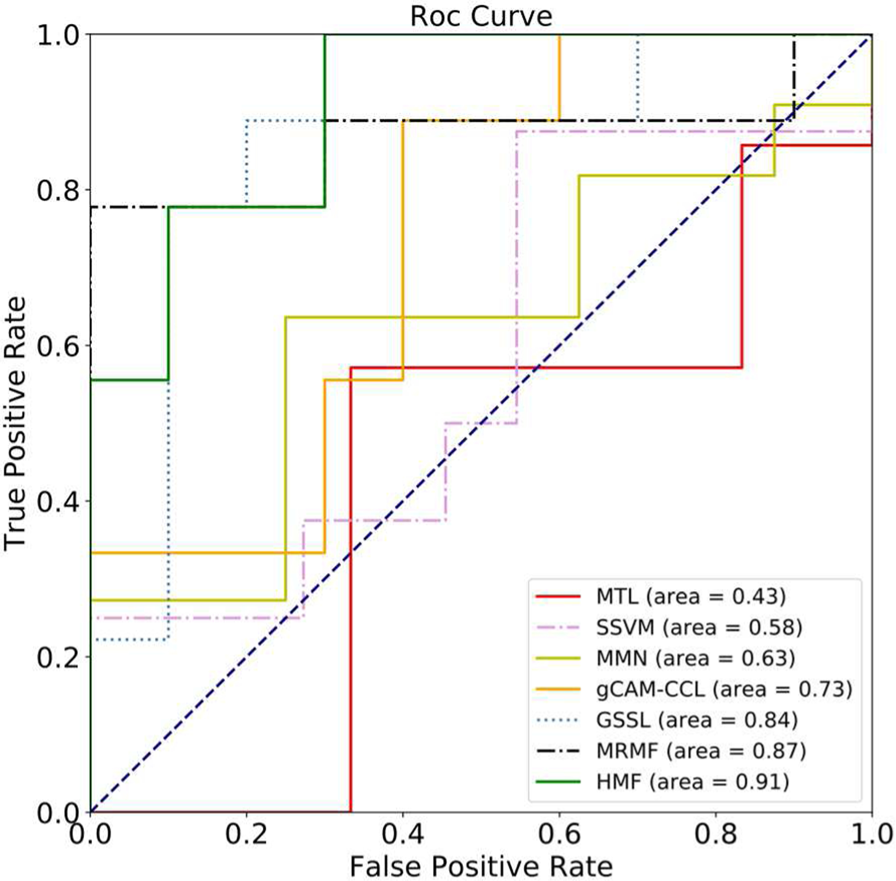
The ROC curves with 7 compared algorithms testing on the MCIC dataset.

C. Discussion

1). Significance of Results:

Our proposed algorithm achieved high performance in schizophrenia classification while identifying a subset of significant features. To facilitate the analysis of these potential biomarkers, we used the features obtained from the real data experiment for further analysis. The feature weights represent their importance to the disease label. Based on the weight vector w estimated by our model, we then investigated the potential of SNP sites, DNA methylation sites and brain ROIs as potential biomarkers associated with schizophrenia, respectively. In addition, the false discovery rate (FDR) is used in multiple hypothesis testing, where the Benjamini–Hochberg (BH) procedure was applied to control the FDR.

Table II lists the top 20 ranked schizophrenia-related SNP sites identified by HMF. Some of the corresponding genes have been reported in the previous works. Specifically, CNTN2 [35], B3GAT1 [43], INSIG2 [44] and ACTG2 [45] have been confirmed to be related to brain development and neural signals. CNTN2 belongs to CNTN family that promotes the outgrowth of neuron and influences neuronal networks in the broad brain areas. In a study by the schizophrenia psychiatric GWAS consortium [46], CSMD1 and C20orf39, as the target of miR-137, have been reported to have genome-wide significant association with SZ. Increased mRNA level of MAN1A1 is identified in [47], which plays an essential role in N-glycan maturation and reflects dysregulated gene expression in schizophrenia of enzymes that participate in many stages of immature N-glycan processing. In addition, inflammation related gene IL1B is indicated to play an important role in the abnormal psychomotor behavior characteristics in SZ [48].

TABLE II.

The Risk Genes Identified by HMF From SNP Data

SNP ID	GENE	p-value
rs10503303	CSMD1	9.14×10−3
rs11224169	B3GAT1	8.14×10−3
rs11164963	BCAR3	8.14×10−3
rs10954922	INSIG2	8.14×10−3
rs11723281	AREG	9.14×10−3
rs10211364	RND3	8.75×10−3
rs11890391	LOC100131409	8.14×10−3
rs10819861	NCRNA00092	8.14×10−3
rs12039496	OLFM3	8.14×10−3
rs10244538	MAN1A1	8.75×10−3
rs11797927	DDX26B	9.14×10−3
rs1009216	IL1B	8.75×10−3
rs10417171	LOC100288860	8.14×10−3
rs11773926	ACTG2	8.75×10−3
rs1105892	NMNAT3	8.14×10−3
rs10305710	CNTN2	8.14×10−3
rs11573653	RAD23B	8.14×10−3
rs11699265	C20orf39	9.14×10−3
rs10960412	DMRT2	8.75×10−3
rs1044085	SFIl	6.34×10−3

Table III lists the top 15 ranked DNA methylation epigenetic factors associated with SZ detected by the HMF, which are in accordance with the previous studies in the literature. For instance, TNRC4 on chromosome 15q11-q13 has been confirmed to cause the imprinting neuro developmental disorder, which may lead affective disorders and psychosis [49]. MTERF controls the mitochondrial transcription termination function, which leads to the clinical manifestations of some mental illness symptoms [50]. As a promising novel candidate gene, DCC is reported in the literature [51] that may contribute to the genetic basis behind individual differences in susceptibility to SZ. The gene encoding Cadherin-13 (CDH13), a cell adhesion molecule, is related to neuropsychiatric conditions [52]. Genes such as PFTK1, TMEM14B, and FLJ40629 are also related to SZ in the literature [35].

TABLE III.

The Risk Genes Identified by HMF From DNA Methylation Data

Index	GENE	p-value
cg00915289	TNRC4	9.13×10−3
cg00160914	MRPS21	9.13×10−3
cg01064307	WERE	8.85×10−3
cg01346152	DCC	8.85×10−4
cg00540544	TP73	8.85×10−3
cg00625425	CDH13’	8.85×10−3
cg00808492	02E6’	9.13×10−3
cg01182697	FLJ40629	9.13×10−3
cg00816620	PTAFR	9.42×10−3
cg00528052	IIP45	9.13×10−3
cg00904574	PFTK1	8.85×10−3
cg00128877	LAMB3	9.13×10−3
cg01045423	PLEKHA6	9.13×10−3
cg00750606	SFPQ	9.13×10−3
cg00208830	TMEM14B	9.13×10−3

Through the analysis of fMRI data, the top 15 ROIs were detected to be related with SZ as shown in Table IV. Some of these detections are also consistent with the results of previous studies, e.g., the differences between SZ patients and healthy controls are mainly located in the Hippocampus, Precuneus and Cerebellum [53], [54], and the ROIs such as Temporal Sup_R, Insula_L and Lingual_L are also found to be abnormal in SZ patients [35], [45]. The gray matter of the left central posterior gyrus (Postcentral_L) is detected to be significantly lower in SZ patients than that of healthy people [55]. It is also mentioned in [53] that the injured brain area of SZ patients is larger than that of healthy people, especially in cerebellum, frontal cortex, thalamus and temporal cortex, and the connection between Superior frontal gyrus and Calcarine cortex has undergone specific changes in the dominant state. These ROIs are also visualized from the axial, the sagittal left and the sagittal right view in Fig. 8 via the BrainNet viewer [56].

TABLE IV.

The ROIs Identified by HMF From fMRI Data

ID	ROI	p-value
40	ParaHippoctunpal_R	9.88×10−3
19	Supp_Motor_Area_L	9.88×10−3
1	Precentral_L	9.40×10−3
106	Cerebellum_9_R	9.40×10−3
24	Frontal_Sup_Medial_R	9.40×10−3
29	Insula_L	9.40×10−3
16	Frontal_Inf_Orb_R	9.40×10−3
7	Frontal_Mid_L	9.40×10−3
57	Postcentral_L	9.40×10−3
26	Frontal_Mid_Orb_R	9.40×10−3
34	Cingulum_Mid_R	9.40×10−3
3	Frontal_Sup_L	9.40×10−3
47	Lingual_L	9.40×10−3
82	Temporal_Sup_R	9.51×10−3
15	Frontal_Inf_Orb_L	9.40×10−3

Fig. 8.

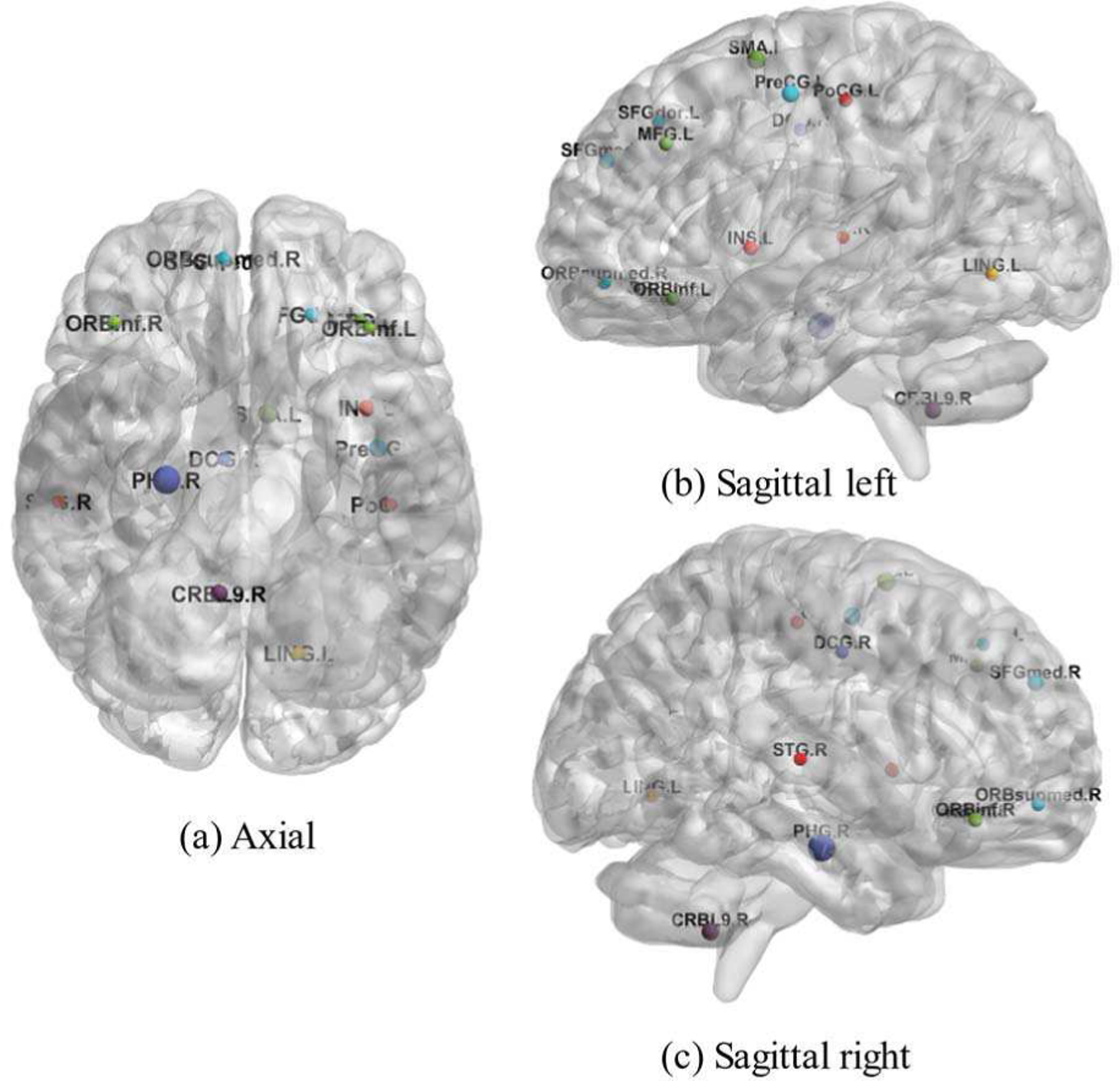
Visualization of 15 abnormal brain ROIs.

To further test the selected genes for over-representation analysis, we performed a pathway enrichment analysis using ConsensusPathDB [57]. The Gene ontology (GO) terms related to neural activity enriched with p-value less than 0.01 are summarized in Table V. For instance, GO terms, including ‘positive regulation of nervous system development,’ ‘central nervous system neuron differentiation,’ ‘brain development,’ ‘regulation of nervous system development’ and ‘regulation of neurogenesis,’ have been proven to be related to SZ [35], [43], [44]. The ‘positive regulation of nervous system development’ pathway is significantly related to the development and formation of neurons, and the dysfunction of the autonomic nervous system in SZ has a major impact on cognitive and metabolic health [58]. The ‘central nervous system neuron differentiation’ pathway and the ‘regulation of neurogenesis’ pathway are closely related to the central nervous system; they indicate that the establishment and maintenance of DNA methylation are crucial in the differentiation of the central nervous system [59], [60]. Furthermore, growing evidence points to synaptic pathology as a core component of the pathophysiology of SZ. This methylation is related to synaptic plasticity, learning and memory, and the disorder of the synaptic network is an important mechanism underlying SZ [61], [62].

TABLE V.

The Enriched Gene Ontology (GO) Terms That Are Related to the Neural Activity

Gene ontology term	p-value
Positive regulation of nervous system development	6.85×10−5
Regulation of synapse structure or activity	5.16×10−3
Regulation of synapse organization	4.52×l0−3
Synapse assembly	2.85×l0−3
Regulation of nervous system development	6.10×10−4
Regulation of synapse assembly	5.08×10−4
Positive regulation of synapse assembly	1.18×l0−4
Central nervous system neuron differentiation	3.81×l0−3
Brain development	7.67×l0−3
Head development	9.64×10−3
Regulation of neurogenesis	3.42×10−4
Positive regulation of synapse assembly	6.85×l0−5

2). Effect of the Regularization Terms:

Through the experiments of both the simulated and real datasets, the effect of the proposed regularization terms as a way of incorporating prior knowledge can be further investigated. In particular, the performances of HMF, MRMF and GSSL are superior to those of other algorithms, i.e., MTL, SNF-SVM, MMN and gCAM-CCL, which indicate that the manifold learning-based regularization terms incorporate structural information in the high dimensional data into the regression model to overcome overfitting problems, resulting in better classification accuracy and are more robust against noise. Since MRMF can be regarded as the graph-based version of HMF, their comparison indicates that employing the high-order structural information can have added values. Similarly, GSSL is a manifold learning-based algorithm that does not consider the subject relationship between different modalities. The comparison between GSSL and MRMF demonstrates that incorporating the subject by subject interactions across multiple modalities can further improve the performance than based only on single modality. Moreover, by testing HMF on different combinations of three datasets, we can show that our model can effectively combine complementary information from multi-modal data, leading to improved classification.

It is worth noting that deep learning-based multi-modal fusion models such as the gCAM-CCL and offer alternative ways for the classification. However, these approaches usually request a large number of samples to train the model. In addition, they are usually complicated to interpret the extracted features. In fact, the classification accuracy of gCAM-CCL on both the simulated and the MICI data is lower than three manifold regularization methods, i.e., GSSL, MRMF and HMF. This may be due to the small sample size that limits the performance of gCAM-CCL. Other deep learning methods such as MGCN [64], a manifold regularized graph convolutional network model, uses features as nodes to construct the graph, which is not applicable to our problem.

In summary, the proposed algorithm employs a joint learning model to take advantage of complementary information from multi-modal data, and incorporates the interactions of subjects both within a single and across multiple modalities into the regression model to overcome the overfitting issue. The validation on both simulated and real data demonstrate its advantage in processing small sample but high dimensional data with robustness to the data noise.

3). Limitations:

However, there are some limitations in our current study. First, this algorithm is still based on linear regression and therefore cannot capture the complex non-linear relationship between imaging genomics markers and phenotypes while multi-modal deep learning model provides a promising direction. Second, in learning the hypergraph, the estimation of incidence matrix is based on the nearest neighbor approach and the hyperedge weight value ψ(e) is set to 1. While this renders the hypergraph easier to learn, we can employ several advanced sparsity learning techniques to compute the weights of the hyperedges, resulting in better characterization of high-order relationships.

IV. Conclusion

In this paper, we proposed a hypergraph-based manifold regularization algorithm to integrate multi-modal imaging genetics data. Specifically, the high-order similarity structure between subjects within a modality and across multiple modalities is constructed by a hypergraph, which is used to design the manifold regularization term. Then, multi-modal data is fused by a multiple regression model enforced with the regularization terms to incorporate prior knowledge from multiple data, which has the advantage in overcoming overfitting issues in high dimensional data analysis. Our algorithm is validated on both simulation and the MCIC dataset for the study of schizophrenia. The experimental results demonstrate that our proposed model achieves superior performance in the classification of schizophrenia compared with other competing models. Moreover, they can be used to identify significant biomarkers in schizophrenia, which are further supported by previous reports.

TABLE I.

The Comparison of Different Algorithms Testing on the MCIC Dataset

Model	Accuracy	RMSE
MTL	0.5470 ± 0.0339	1.3072 ± 0.2123
SNF-SVM	0.5783 ± 0.0301	0.9331 ± 0.1937
MMN	0.6942 ± 0.0363	0.8646 ± 0.1749
GSSL	0.8202 ± 0.0217	0.7884 ± 0.1573
gCAM-CCL	0.7721 ± 0.0224	0.7945 ± 0.1184
MRMF	0.8479 ± 0.0162	0.7342 ± 0.0126
HMF	0.8749 ± 0.0164	0.6902 ± 0.1053

References

- [1].Lahat D, Adali T and Jutten C, “Multimodal Data Fusion: An Overview of Methods, Challenges, and Prospects,”Proceedings of the IEEE, vol. 103, no. 9, pp. 1449–1477, Sept. 2015. [Google Scholar]
- [2].Rashid B and Calhoun VD, “Towards a brain - based predictome of mental illness,” Human brain mapping, vol. 41, no. 12, pp. 3468–3535, Aug. 2020. [DOI] [PMC free article] [PubMed] [Google Scholar]
- [3].Adali T, Levin-Schwartz Y and Calhoun VD, “Multimodal Data Fusion Using Source Separation: Application to Medical Imaging,” Proceedings of the IEEE, vol. 103, no. 9, pp. 1494–1506, Sept. 2015. [DOI] [PMC free article] [PubMed] [Google Scholar]
- [4].Li Y, Yang M and Zhang Z, “A Survey of Multi-View Representation Learning,” IEEE Transactions on Knowledge and Data Engineering, vol. 31, no. 10, pp. 1863–1883, 1 Oct. 2019. [Google Scholar]
- [5].Calhoun VD and Sui J, “Multimodal Fusion of Brain Imaging Data: A Key to Finding the Missing Link(s) in Complex Mental Illness,” Biological psychiatry: cognitive neuroscience and neuroimaging, vol. 1, no. 3, pp. 230–244, Jan. 2016. [DOI] [PMC free article] [PubMed] [Google Scholar]
- [6].Sui J, Adali T, Yu Q et al. , “A Review of Multivariate Methods for Multimodal Fusion of Brain Imaging Data,” Journal of neuroscience methods, vol. 204, no. 1, pp. 68–81, Feb. 2012. [DOI] [PMC free article] [PubMed] [Google Scholar]
- [7].Groves AR, Beckmann CF, Smith SM et al. , “Linked independent component analysis for multimodal data fusion,” Neuroimage, vol. 54, no. 3, pp. 2198–2217, Feb. 2011. [DOI] [PubMed] [Google Scholar]
- [8].Gao J, Li P, Chen Z et al. , “A Survey on Deep Learning for Multimodal Data Fusion,” Neural Computation, vol. 32, no. 5, pp. 829–864, March 2020. [DOI] [PubMed] [Google Scholar]
- [9].Robert T, “Regression shrinkage and selection via the lasso,” Journal of the Royal Statistical Society: Series B (Methodological), vol. 58, no. 1, pp. 267–288, 1996. [Google Scholar]
- [10].Fu WJJ, “Penalized regressions: the bridge versus the lasso,” Journal of computational and graphical statistics, vol. 7, no. 3, pp. 397–416, 1998. [Google Scholar]
- [11].Zou H and Hastie T, “Regularization and variable selection via the elastic net,” Journal of the royal statistical society: series B (statistical methodology), vol. 67, no. 2, pp. 301–320, 2005. [Google Scholar]
- [12].Yuan M and Yi L, “Model selection and estimation in regression with grouped variables,” Journal of the Royal Statistical Society: Series B (Statistical Methodology), vol. 68, no. 1, pp. 49–67, 2006. [Google Scholar]
- [13].Holger H, “A path algorithm for the fused lasso signal approximator,” Journal of Computational and Graphical Statistics, vol. 19, no. 4, pp. 984–1006, 2010. [Google Scholar]
- [14].Chuang HY et al. , “Network-based classification of breast cancer metastasis,” Molecular systems biology, vol. 3, no. 1, pp. 140, 2007. [DOI] [PMC free article] [PubMed] [Google Scholar]
- [15].Huang Y and Pei W, “Network based prediction model for genomics data analysis,” Statistics in biosciences, vol. 4, no. 1, pp. 47–65, 2012. [DOI] [PMC free article] [PubMed] [Google Scholar]
- [16].Kim SK, Wei P and Shen XT, “Network-based penalized regression with application to genomic data,” Biometrics, vol. 69, no. 3, pp. 582–593, 2013. [DOI] [PMC free article] [PubMed] [Google Scholar]
- [17].Liu JY and Calhoun VD, “A review of multivariate analyses in imaging genetics,” Frontiers in neuroinformatics, vol. 8, pp. 29, 2014. [DOI] [PMC free article] [PubMed] [Google Scholar]
- [18].Lei BY et al. , “Neuroimaging retrieval via adaptive ensemble manifold learning for brain disease diagnosis,” IEEE journal of biomedical and health informatics, vol. 23, no. 4, pp. 1661–1673, 2018. [DOI] [PubMed] [Google Scholar]
- [19].Adeli E, Meng Y, Li G et al. , “Multi-task prediction of infant cognitive scores from longitudinal incomplete neuroimaging data,” Neuroimage, vol. 185, pp. 783–792, Jan. 2019. [DOI] [PMC free article] [PubMed] [Google Scholar]
- [20].Jie B, Zhang D, Cheng B et al. , “Manifold regularized multitask feature learning for multimodality disease classification,” Human brain mapping, vol. 36, no 2, pp. 489–507, Feb. 2015. [DOI] [PMC free article] [PubMed] [Google Scholar]
- [21].Zhu X, Suk H, Lee S and Shen D, “Subspace Regularized Sparse Multitask Learning for Multiclass Neurodegenerative Disease Identification,” IEEE Transactions on Biomedical Engineering, vol. 63, no. 3, pp. 607–618, March 2016. [DOI] [PMC free article] [PubMed] [Google Scholar]
- [22].Du L et al. , “Multi-Task Sparse Canonical Correlation Analysis with Application to Multi-Modal Brain Imaging Genetics,” IEEE/ACM Transactions on Computational Biology and Bioinformatics, vol. 18, no. 1, pp. 227–239, 1 Jan.-Feb. 2021. [DOI] [PMC free article] [PubMed] [Google Scholar]
- [23].Bai Y, Pascal Z, Calhoun V and Wang Y-P, “Optimized Combination of Multiple Graphs with Application to the Integration of Brain Imaging and (epi) Genomics Data,” IEEE Transactions on Medical Imaging, vol. 39, no. 6, pp. 1801–1811, June 2020. [DOI] [PMC free article] [PubMed] [Google Scholar]
- [24].Liu Y, Fan L, Zhang C et al. , “Incomplete multi-modal representation learning for Alzheimer’s disease diagnosis,” Medical Image Analysis, vol. 69, pp. 101–953, Apr. 2021. [DOI] [PubMed] [Google Scholar]
- [25].Hu W et al. , “Interpretable Multimodal Fusion Networks Reveal Mechanisms of Brain Cognition,” IEEE Transactions on Medical Imaging, vol. 40, no. 5, pp. 1474–1483, May 2021. [DOI] [PMC free article] [PubMed] [Google Scholar]
- [26].Zhang Y et al. , “Multi-Paradigm fMRI Fusion via Sparse Tensor Decomposition in Brain Functional Connectivity Study,” IEEE Journal of Biomedical and Health Informatics, vol. 25, no. 5, pp. 1712–1723, May 2021. [DOI] [PMC free article] [PubMed] [Google Scholar]
- [27].Xiao L, Stephen JM, Wilson TW, Calhoun VD and Y. -P. Wang, “A Manifold Regularized Multi-Task Learning Model for IQ Prediction From Two fMRI Paradigms,” IEEE Transactions on Biomedical Engineering, vol. 67, no. 3, pp. 796–806, March 2020. [DOI] [PMC free article] [PubMed] [Google Scholar]
- [28].Gollub RL, Shoemaker JM, King MD et al. “The MCIC Collection: A Shared Repository of Multi-Modal, Multi-Site Brain Image Data from a Clinical Investigation of Schizophrenia,” Neuroinformatics vol. 11, no. 3, pp. 367–388, July 2013. [DOI] [PMC free article] [PubMed] [Google Scholar]
- [29].Ji R, Gao Y, Hong R, Liu Q, Tao D and Li X, “Spectral-Spatial Constraint Hyperspectral Image Classification,” IEEE Transactions on Geoscience and Remote Sensing, vol. 52, no. 3, pp. 1811–1824, March 2014. [Google Scholar]
- [30].Xiao L et al. , “Multi-Hypergraph Learning-Based Brain Functional Connectivity Analysis in fMRI Data,” IEEE Transactions on Medical Imaging, vol. 39, no. 5, pp. 1746–1758, May 2020. [DOI] [PMC free article] [PubMed] [Google Scholar]
- [31].Zhou D, Huang J and Schölkopf B, “Learning with Hypergraphs: Clustering, Classification, and Embedding,” Advances in neural information processing systems, vol. 19, pp. 1601–1608, Jan. 2006. [Google Scholar]
- [32].W Shao Y Peng, C Zu et al. , “Hypergraph Based Multi-task Feature Selection for Multimodal Classification of Alzheimer’s Disease” Computerized Medical Imaging and Graphics, vol. 80, 101663, June 2020. [DOI] [PubMed] [Google Scholar]
- [33].Sa VD, “Spectral clustering with two views,” in ICML workshop on learning with multiple views, pp. 20–27, 2005.
- [34].Lindenbaum O, Yeredor A, Salhov M et al. “Multi-view Diffusion Maps” Information Fusion, vol. 55, pp. 127–149, Mar. 2020. [Google Scholar]
- [35].Hu W et al. , “Adaptive Sparse Multiple Canonical Correlation Analysis with Application to Imaging (Epi)Genomics Study of Schizophrenia,” IEEE Transactions on Biomedical Engineering, vol. 65, no. 2, pp. 390–399, Feb. 2018. [DOI] [PMC free article] [PubMed] [Google Scholar]
- [36].Evgeniou A and Pontil M, “Multi-task feature learning,” in Advances in neural information processing systems, British, Columbia: Vancouver, Canada, 2007, pp. 19–41. [Google Scholar]
- [37].B Wang A Mezlini M, Demir F et al. “Similarity network fusion for aggregating data types on a genomic scale,” Nature methods, vol. 11, no. 3, pp. 333–337, Mar. 2014. [DOI] [PubMed] [Google Scholar]
- [38].Deng S, Hu W, Calhoun VD et al. “Schizophrenia Prediction Using Integrated Imaging Genomic Networks”Advances in Science, Technology and Engineering Systems, vol. 2, no. 3, pp. 702–710, June 2017. [Google Scholar]
- [39].Tzourio-Mazoyer N, Landeau B, Papathanassiou D et al. “Automated Anatomical Labeling of Activations in SPM Using a Macroscopic Anatomical Parcellation of the MNI MRI Single-Subject Brain” Neuroimage, vol. 15, no. 1, pp. 273–289, Jan. 2002. [DOI] [PubMed] [Google Scholar]
- [40].Pidsley R et al. , “A data-driven approach to preprocessing Illumina 450K methylation array data,” BMC genomics, vol. 14, no. 1, pp. 1–10, May 2013. [DOI] [PMC free article] [PubMed] [Google Scholar]
- [41].Liu J, Chen J, Ehrlich S et al. “Methylation patterns in whole blood correlate with symptoms in schizophrenia patients,” Schizophrenia bulletin, vol. 40, no. 4, pp. 769–776, July 2014. [DOI] [PMC free article] [PubMed] [Google Scholar]
- [42].Lin D, Calhoun VD and Wang YP, “Correspondence between fMRI and SNP data by group sparse canonical correlation analysis,” Medical image analysis, vol. 18, no 6, pp. 891–902, Aug. 2014. [DOI] [PMC free article] [PubMed] [Google Scholar]
- [43].Fang J, Lin D, Schulz SC et al. “Joint sparse canonical correlation analysis for detecting differential imaging genetics modules,”Bioinformatics, vol. 32, no. 22, pp. 3480–3488, Nov. 2016. [DOI] [PMC free article] [PubMed] [Google Scholar]
- [44].Peng P et al. , “Group Sparse Joint Non-negative Matrix Factorization on Orthogonal Subspace for Multi-modal Imaging Genetics Data Analysis,” IEEE/ACM Transactions on Computational Biology and Bioinformatics, to be published. DOI: 10.1109/TCBB.2020.2999397. [DOI] [PMC free article] [PubMed]
- [45].Wang M, Huang T-Z, Fang J, Calhoun VD and Wang Y-P, “Integration of Imaging (epi) Genomics Data for the Study of Schizophrenia Using Group Sparse Joint Nonnegative Matrix Factorization,” IEEE/ACM Transactions on Computational Biology and Bioinformatics, vol. 17, no. 5, pp. 1671–1681, 1 Sept.-Oct. 2020. [DOI] [PMC free article] [PubMed] [Google Scholar]
- [46].Kwon E, Wang W and Tsai LH, “Validation of schizophrenia-associated genes CSMD1, C10orf26, CACNA1C and TCF4 as miR-137 targets” Molecular psychiatry, vol. 18, no. 1, pp. 11–12, Jan. 2013. [DOI] [PubMed] [Google Scholar]
- [47].Mueller TM Simmons MS, Helix AT et al. , “Glycosylation enzyme mRNA expression in dorsolateral prefrontal cortex of elderly patients with schizophrenia: Evidence for dysregulation of multiple glycosylation pathways,” BioRxiv: 369314, July 2018.
- [48].Zhang Y, You X, Li S et al. “Peripheral Blood Leukocyte RNA-Seq Identifies a Set of Genes Related to Abnormal Psychomotor Behavior Characteristics in Patients with Schizophrenia,” Medical science monitor: international medical journal of experimental and clinical research, vol. 26, pp. e922426–1–e922426–31, Feb. 2013. [DOI] [PMC free article] [PubMed] [Google Scholar]
- [49].Samaan MC, “Prader-Willi Syndrome: Genetics, Phenotype, and Management,” in Current Psychiatry Reviews, vol. 1, no. 2, pp. 168–181, June 2014. [Google Scholar]
- [50].Ann G, “Psychiatric disorders, mitochondrial dysfunction, and somatotypes” Ros Vestn Perinatol Pediat, vol. 4, no. 2, pp. 70–75, Jan. 2012. [Google Scholar]
- [51].Grant A, Fathalli F, Rouleau G et al. “Association between schizophrenia and genetic variation in DCC: A case–control study,” Schizophrenia research, vol. 137, no. 1–3, pp. 26–31, May 2012 [DOI] [PubMed] [Google Scholar]
- [52].Rivero O, Sich S, Popp S et al. “Impact of the ADHD-susceptibility gene CDH13 on development and function of brain networks,” European Neuropsychopharmacology, vol. 23, no. 6, pp. 492–507, June 2013 [DOI] [PubMed] [Google Scholar]
- [53].Du Y, Fryer SL, Fu Z et al. “Dynamic functional connectivity impairments in early schizophrenia and clinical high-risk for psychosis,” Neuroimage, vol. 180, pp. 632–645, Oct. 2018 [DOI] [PMC free article] [PubMed] [Google Scholar]
- [54].Duan H, Gan J, Yang J et al. “A longitudinal study on intrinsic connectivity of hippocampus associated with positive symptom in first-episode schizophrenia,” Behavioural brain research, vol. 283, pp. 78–86, June 2015 [DOI] [PubMed] [Google Scholar]
- [55].Job DE, Whalley HC, McConnell S et al. “Structural Gray Matter Differences between First-Episode Schizophrenics and Normal Controls Using Voxel-Based Morphometry,” Neuroimage, vol. 17 no. 2, pp. 880–889, June 2002 [PubMed] [Google Scholar]
- [56].Xia M, Wang J and He Y. “BrainNet Viewer: a network visualization tool for human brain connectomics,”PloS one, vol. 8, no. 7, June 2013. [DOI] [PMC free article] [PubMed] [Google Scholar]
- [57].Kamburov A, Stelzl U, Lehrach H et al. “The ConsensusPathDB interaction database: 2013 update” Nucleic acids research, vol. 41, no. D1, pp. D793–D800, Jan. 2013. [DOI] [PMC free article] [PubMed] [Google Scholar]
- [58].Stogios N, Gdanski A, Gerretsen P et al. “Autonomic nervous system dysfunction in schizophrenia: impact on cognitive and metabolic health,” NPJ schizophrenia, vol. 7, no. 1, pp. 1–10, Apr. 2021. [DOI] [PMC free article] [PubMed] [Google Scholar]
- [59].Tao R, Li C, Jaffe AE et al. “Cannabinoid receptor CNR1 expression and DNA methylation in human prefrontal cortex, hippocampus and caudate in brain development and schizophrenia,” Translational psychiatry, vol. 10, no. 1, pp. 1–13, May 202. [DOI] [PMC free article] [PubMed] [Google Scholar]
- [60].Grayson DR and Guidotti A, “The Dynamics of DNA Methylation in Schizophrenia and Related Psychiatric Disorders,” Neuropsychopharmacology, vol. 38, no. 1, pp. 138–166, Jan. 2013. [DOI] [PMC free article] [PubMed] [Google Scholar]
- [61].Berlekom A, Muflihah CH, Snijders G, et al. “Synapse Pathology in Schizophrenia: A Meta-analysis of Postsynaptic Elements in Postmortem Brain Studies,” Schizophrenia Bulletin, vol. 46, no. 5, pp. 374–386, June 2019. [DOI] [PMC free article] [PubMed] [Google Scholar]
- [62].Chelini G et al. , “The tetrapartite synapse: A key concept in the pathophysiology of schizophrenia,” European psychiatry: the journal of the Association of European Psychiatrists, vol. 50, pp. 60–69, Apr. 2018. [DOI] [PMC free article] [PubMed] [Google Scholar]
- [63].Gao Y, Wang M, Tao D, Ji R and Dai Q, “3-D Object Retrieval and Recognition with Hypergraph Analysis,”IEEE Transactions on Image Processing, vol. 21, no. 9, pp. 4290–4303, Sept. 2012 [DOI] [PubMed] [Google Scholar]
- [64].Qu G et al. , “Ensemble manifold regularized multi-modal graph convolutional network for cognitive ability prediction,” IEEE Transactions on Biomedical Engineering, to be published. DOI: 10.1109/TBME.2021.3077875 [DOI] [PubMed]
- [65].Friedman J, Hastie T and Tibshirani R, “Sparse inverse covariance estimation with the graphical lasso.” Biostatistics, vol. 9, no. 3, pp. 432–441, July 2008. [DOI] [PMC free article] [PubMed] [Google Scholar]
- [66].Yu G and Liu Y “Sparse regression incorporating graphical structure among predictors.” Journal of the American Statistical Association, vol. 111, no. 514, pp. 707–720, Aug. 2016. [DOI] [PMC free article] [PubMed] [Google Scholar]
- [67].Danaher P, Wang P, and Witten DM “The joint graphical lasso for inverse covariance estimation across multiple classes.” Journal of the Royal Statistical Society. Series B, Statistical methodology, vol. 76, no. 2, pp. 373–397, Mar. 2014. [DOI] [PMC free article] [PubMed] [Google Scholar]
- [68].Hou C et al. , “Learning high-dimensional correspondence via manifold learning and local approximation.” Neural Computing and Applications, vol. 24, no. 7, pp. 1555–1568, Mar. 2013. [Google Scholar]
- [69].Cao X et al., “Selecting key poses on manifold for pairwise action recognition.” IEEE Transactions on Industrial Informatics, vol. 8, no. 1, pp. 168–177, Oct. 2011. [Google Scholar]