Deep cross-modality (MR-CT) educed distillation learning for cone beam CT lung tumor segmentation

Abstract

Purpose:

Despite the widespread availability of in-treatment room cone beam computed tomography (CBCT) imaging, due to low soft-tissue contrast and the effort needed for manual delineation, CBCT is only used for qualitative tumor response assessment and gross set up corrections in lung radiotherapy. Accurate and reliable segmentation tools could potentiate quantitative response assessment and geometry-guided adaptive radiotherapy. Therefore, we developed a new deep learning CBCT lung tumor segmentation method.

Methods:

The key idea of our approach called cross modality educed distillation (CMEDL) is to use more informative magnetic resonance imaging (MRI) to constrain the CBCT segmentation features extracted from a network during training. We accomplish this by training an end-to-end network comprised of unpaired domain adaptation (UDA) and cross-domain segmentation distillation networks (SDN) using unpaired CBCT and MRI datasets. Unpaired domain adaptation means that the CBCT and MRI are not aligned and may arise from different sets of patients. The UDA network synthesizes pseudo MRI from CBCT images. The SDN consists of teacher MRI and student CBCT segmentation networks. Feature distillation is done by constraining the student network to extract features matching the teacher network. Thus, the student CBCT network learns to extract features that maximize the contrast between the target and the background like the teacher network, which uses more informative MRI images. The UDA network was implemented with a cycleGAN improved with contextual losses. We evaluated both Unet and dense fully convolutional segmentation networks (DenseFCN). Performance comparisons were done against CBCT only networks. We also compared against an alternative framework that used UDA with MR segmentation network, whereby segmentation was done on the synthesized pseudo MRI representation. All networks were trained with identical datasets using three fold cross-validation from 43 CBCT and 82 T2W turbo spin echo MRIs. Testing was done on additional 51 CBCTs. Performance was assessed using surface Dice similarity coefficient (SDSC) and Hausdroff distance at 95th percentile (HD95) metrics.

Results:

The CMEDL approach significantly improved (p < 0.001) the accuracy of both Unet (SDSC of 0.83 ± 0.08; HD95 of 7.69 ± 7.86mm) and DenseFCN (SDSC of 0.75 ± 0.13; HD95 of 11.42 ± 9.87mm) over CBCT only Unet (SDSC of 0.69 ± 0.11; HD95 of 21.70 ± 16.34mm) and DenseFCN (SDSC of 0.66 ± 0.15; HD95 of 22.15 ± 17.19mm) networks. The alternate framework using UDA with the MRI network was also more accurate than the CBCT only methods but less accurate than the CMEDL approach.

Conclusion:

Our results demonstrate that the introduced CMEDL approach produces reasonably accurate lung cancer segmentation from CBCT images. Further validation on larger datasets is necessary for clinical translation.

I. INTRODUCTION

Lung cancer is the leading cause of cancer-related deaths in both men and women in the United States[1]. The standard treatment for inoperable or unresectable stage III cancers is definitive/curative radiotherapy to 60 Gy in 30 fractions with concomittant chemotherapy[2]. Recently, dose escalation trials and high-dose adaptive radiotherapies[3, 4] have shown the feasibility to improve local control and survival in locally advanced non-small cell lung cancer (LA-NSCLC). However, a key technical challenge in delivering high-dose treatments, both at the time of planning and delivery is accurate and precise delineation of both target tumors and normal organs[5].

Importantly, X-ray cone beam CT (CBCT) imaging is available as part of standard equipment. However, much of the in-treatment-room CBCT information cannot be used routinely beyond basic positioning corrections. In fact, a key obstacle for clinical adoption of adaptive radiotherapy for LA-NSCLC is the lack of reliable segmentation tools, needed for geometric corrections in target and possibly the critical OARs[4, 6]. Despite the widespread development of deep learning segmentation methods, to our best knowledge, there are no reliable CBCT methods for routine lung cancers treatment. The latest works published were primarily focused on the pelvic regions for prostate cancer radiotherapy[7, 8].

The difficulty in generating accurate segmentation results from the lack of sufficient soft-tissue contrast on CBCT imaging, especially in the mediastinum region. A consequence of low soft-tissue contrast is the inherent difficulty in extracting features that clearly differentiate the segmented target from its background structures even for a deep learning method. Prior work by[8] has shown that performing segmentation on an image representation like pseudo MRI images that contain better soft tissue contrast information than the CBCT itself can lead to improved performance. Our approach uses the key insight that a more informative modality like magnetic resonance imaging (MRI) with better soft-tissue contrast can be used to constrain the features used to perform inference on less informative CBCT modality. Unlike the approach in[8] that required paired sets of CT and MRI images, our approach uses unpaired CBCT and MRI images, which are easier to obtain and practically applicable without requiring specialized imaging protocols for algorithm development.

Our approach introduces unpaired cross-modality distillation learning. Distillation learning was introduced to compress the knowledge contained in an information rich, high-capacity network (trained with a large training data) into a small, low-capacity network[9], using paired images. Model compression is meaningful when a high-capacity model is not required for a task or the computational limitation of using such a large classifier necessitates the use of simpler and computationally fast model [10] for real-time analysis. The approach in[9] used same modality images and was used to solve different image-based classification tasks. Distillation itself was done by using the probabilistic ”softMax” outputs of the teacher as target output for the student (compressed) network. Improvements to this approach included hint learning where features from intermediate layers in the student network are constrained to mimic the features from the teacher network [11, 12] for image-based classification. Recent works in computer vision, extended this approach using low- and high-resolution images[13], as well as for different modality distillation between paired (Red, Green, Blue) or RGB and depth images[14] for semantic segmentation. Our work extends this approach to unpaired distillation learning using explicit hints between MRI and CBCT images. Also, we modify how the knowledge distillation is employed, whereby instead of transferring knowledge from a very deep network into a smaller network, the teacher and student networks are identical except for the imaging modalities used to train them. The teacher network is trained with a more informative MRI modality, while the student CBCT network is constrained to extract features for inference like the teacher network. As a result, only the CBCT segmentation network is required for testing. Prior CBCT method[8] requires both cross-modality I2I translation and the segmentation network at testing time.

This work builds on our prior work that used unpaired MRI and contrast enhanced CT (CECT) datasets to improve CECT lung tumor segmentation[15]. Our approach called cross-modality educed distillation learning (or CMEDL) extends this approach to more challenging CBCT images. We tested the hypothesis that MRI information extracted using unpaired CBCT and MRI can constrain the features computed from CBCT network and improve performance over CBCT only segmentation. Because the distillation learning framework provides additional constraints in an end-to-end trained network, these losses inform both CBCT segmentation and I2I translation. In[8], the MR segmentation network was directly used for inference by using an I2I translated pseudo MRI produced with a standard cycleGAN[16]. But this approach requires both the I2I translation and the segmentation network at testing time. We evaluated this alternative framework using our CMEDL framework as well as with more advanced variational auto-encoder unsupervised image translation (UNIT)[17] used in place of a cycleGAN[16] network.

Our contributions include: (i) a new unpaired cross-modality educed distillation-based segmentation framework that uses the idea of constraining inference information extracted from less informative modality from a more informative modality, (ii) application of this framework to the challenging CBCT lung tumor segmentation, and (iii) implementation of our framework using two different segmentation networks, with performance comparisons done against other related approaches.

II. MATERIALS AND METHODS

A. Patient and image characteristics

The CBCT dataset came from a combination of internal cohort of 49 LA-NSCLC patients and an external institution cohort[18] of 20 patients with scans acquired every week (6 to 7) during conventionally fractionated radiotherapy. The internal CBCT scans were acquired for routinely monitoring geometric changes of tumor in response to radiotherapy. The external institution 4D CBCT scans were orginally collected for investigating breathing patterns of LA-NSCLC patients undergoing chemoradiotherapy. We only utilized the week one CBCT scan from the external institution dataset. Image resolution for planning 4DCT and weekly 4DCBCT were 0.98 to 1.17 mm in-plane spacing and 3mm slice thickness.

Each CBCT image was standardized and normalized using its global mean and standard deviation, followed by histogram standardization pre-processing and then registered to the planning CT scans using a multi-resolution B-spline regularized diffeomorphic image registration[19, 20]. All contours were reviewed by a radiation oncologist and modified when necessary and served as expert delineation. B-spline registration was performed using a mesh size of 32mm at the coarsest level and was reduced by a factor of two at each sequential level. The optimization step was set to 0.2 with the number of iterations (100, 70, 30) at each level. Additional details of this registration for these datasets are in[20].

Eighty one T2-weighted turbo spin echo (TSE) MRI for cross-modality learning was obtained from 28 stage II-III LA-NSCLC patients scanned every week on a 3T Philips Ingenia scanner. Eleven out of these 28 had weekly MRI scans ranging between 6 to 7 weeks. Seven of these 11 patients overlapped with the internal MSK CBCT cohort. However, the MRI and CBCT images were neither co-registered nor treated as paired image sets for the purpose of training. The MRI scan parameters were: 16-element phased array anterior coil and a 44-element posterior coil (TE/TR = 120/3000-6000ms, slice thickness of 2.5mm, in-plane pixel size of 1.1 × 0.97mm², flip angle of 90^deg, number of averages = 2, and field of view of 300 × 222 × 150mm³.

B. Approach

An overview of our cross-modality educed distillation (CMEDL) approach is shown in Fig. 1. The end-to-end trained network consists of an unpaired cross-domain adaptation (UDA) network composed of a generational adversarial network (GAN)[21] and a segmentation distillation network (SDN), which includes a teacher MRI and student CBCT segmentation network. The teacher network is trained with expert segmented MRI and pseudo MRI images while the CBCT network is trained with expert-segmented CBCT images. Feature distillation is performed by hint learning[11], whereby feature activations on the CBCT network in specific layers (last and penultimate) are forced to mimic the corresponding layer feature activations of the teacher network. Feature activations are matched for corresponding sets of CBCT and synthesized pseudo MRI images.

FIG. 1:

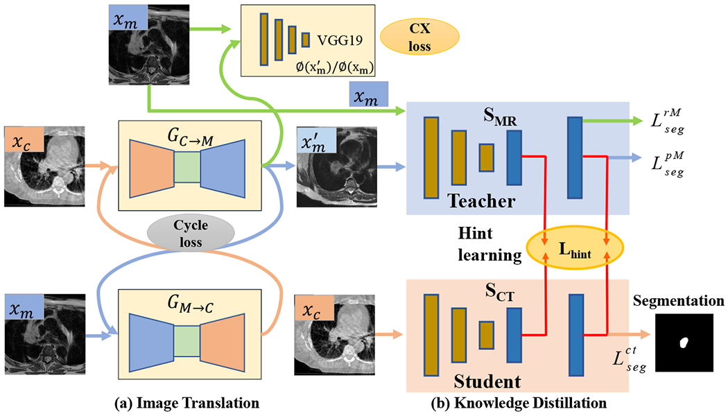
Approach overview. x_c, x_m are the CBCT and MR images from unrelated patient sets; G_C→M and G_M→C are the CBCT and MRI translation networks; $x_m^{\prime }$ is the pseudo MRI (pMRI) image; $x_c^{\prime }$ is the pseudo CBCT image; S_MR is the teacher network; S_CT is the student CBCT segmentation network; CX loss is contextual loss. $L_{seg}^{rM},L_{seg}^{pM}$ are segmentation losses used to train the teacher network, while $L_{seg}^{ct}$ is the loss for the student CBCT network.

C. Notations

The network is trained using a set of expert-segmented CBCT {x_c, y_c} ∈ {X_C, Y_C} and MRI {x_m, y_m} ∈ {X_M, Y_M} datasets. The CBCT and MRI do not have to arise from the same sets of patients and are not aligned for network training. The cross-modality adaptation network consists of generators G_C→M : x_c ↦ x_m to produce pseudo MRI $x_m^{\prime },G_{M\to C}:x_m\mapsto x_c$ to produce pseudo CT images $x_c^{\prime }$, and domain discriminators D_M and D_C. The sub-networks G_M→C and D_C are used to enforce cyclically consistent transformation when using unpaired CBCT and MRI datasets. Feature vectors produced through a mapping function F(x) : x ↦ f(x) are indicated using italized text f_j, where j = 1, … K, for K = H × W × C for 2D and K = H × W × Z × C for 3D, is the number of features for an image of height H, width W, depth Z, and channels C.

D. Stage I: Unpaired cross-domain adaptation for image-to-image translation

The UDA network is composed of a pair of GANs for producing pseudo MRI $x_m^{\prime }$ and pseudo CT $x_c^{\prime }$ images using generator networks G_C→M and G_M→C, respectively. The images produced by these generators are constrained by global intensity discriminators D_M and D_C for MRI and CBCT images, respectively. The adversarial loss for these two networks are computed as:

$$\begin{array}{l}{L}_{adv}^M\left(G_{C\to M},D_M,X_M,X_C\right)={𝔼}_{x_{\text{m}}\sim X_M}\left[\mathit{log}\left(D_M\left(x_m\right)\right)\right]+{𝔼}_{x_c\sim X_C}[\mathit{log}(1-\left(D_M\left(G_{C\to M}\left(x_c\right)\right)\right]\\ L_{adv}^C\left(G_{M\to C},D_C,X_C,X_M\right)={𝔼}_{x_{\text{c}}\sim X_C}\left[\mathit{log}\left(D_C\left(x_c\right)\right)\right]+{𝔼}_{x_m\sim X_M}[\mathit{log}(1-\left(D_C\left(G_{M\to C}\left(x_m\right)\right)\right].\end{array}$$ (1)

Because the networks are trained with unpaired images, cyclical consistency is enforced to shrink the space of possible mappings computed by the generator networks. The loss to enforce this constraint is computed by minimizing the pixel-to-pixel loss (e.g. L1-norm) between the generated (e.g. G_↺M = GM → C(G_C→M(x_c))) and original images as:

$$L_{cyc}\left(G_{C\to M},G_{M\to C},X_c,X_m\right)={𝔼}_{x_c\sim X_c}\left[{\Vert G_{C\circlearrowleft M}\left(x_c\right)-x_c\Vert }_1\right]+{𝔼}_{x_m\sim X_m}\left[{\Vert G_{M\circlearrowleft C}\left(x_m\right)-x_m\Vert }_1\right].$$ (2)

However, the cyclical consistency loss alone can only preserve global statistics while failing to preserve organ or target specific constraints[22]. Furthermore, when performing unpaired adaptation between unaligned images, pixel-to-pixel matching losses are inadequate to preserve spatial fidelity of the structures [23]. Therefore, we used the contextual loss that was introduced in[23]. The contextual loss is computed by matching the low- or mid-level features extracted from the generated and the target images using a pre-trained network like the VGG16[24] (default network used in this work). This loss is computed by treating the features as a collection and by computing all feature-pair similarities, thereby, ignoring the spatial locations. In other words, the similarity between the generated (f(G(x_c)) = g_j) and target feature maps (f(x_m) = m_i) are marginalized over all feature pairings and the maximal similarity is taken as the similarity between those two images. Therefore, this loss also considers the textural aspects of images when computing the generated to target domain matching. It is similar to perceptual losses, but ignores the spatial alignment of these images, which is advantageous when comparing non-corresponding target and source modality generated images. The contextual similarity is computed by normalizing the inverse of cosine distances between the features g_j and m_i as:

$$CX(g,m)=\frac{1}{N}\sum _j\underset{i}{\mathit{max}}CX(g_j,m_i),$$ (3)

where, N corresponds to the number of features. The loss is computed as:

$$L_{cx}=-\mathit{log}(CX\left(f\left(G\left(x_c\right)\right),f\left(x_m\right)\right).$$ (4)

The pseudo MRI images produced through I2I translation from this stage are used in the distillation learning as described below.

E. Stage II: Cross-modality distillation-based segmentation

This stage consists of a teacher (or MRI) segmentation and a student (or CBCT) segmentation network. The goal of distillation learning is to provide hints to the student network such that features extracted in specific layers of the student network match the feature activations for those same layers in the teacher network.

Both teacher (S_M) and student (S_C) networks use the same network architecture (Unet is the default architecture), but process different imaging modalities. Both networks are trained from scratch. The teacher network is trained using expert segmented T2w TSE MRI ({x_m, y_m ∈ {X_M, Y_M}) and pseudo MRI datasets $\left(\left\{x_m^{\prime },y_c\right\}\in \left\{X_C,Y_C\right\}\right)$ obtained from expert-segmented CBCT datasets. The CBCT network is trained with the expert-segmented CBCT datasets. The two networks are optimized using Dice overlap loss:

$$\begin{array}{l}{L}_{\mathit{seg}}=L_{\mathit{seg}}^M+L_{\mathit{seg}}^C\\ ={𝔼}_{x_m\sim X_M}\left[-\mathit{log}P\left(y_m\mid S_M\left(x_m\right)\right)\right]+{𝔼}_{x_m^{\prime }\sim G_{C\to M}\left(X_C\right)}\left[-\mathit{log}P\left(y_c\mid S_M\left(x_m^{\prime }\right)\right)\right]+{𝔼}_{x_c\sim X_C}\left[-\mathit{log}P\left(y_c\mid S_C\left(x_c\right)\right)\right].\end{array}$$ (5)

Feature distillation is performed by matching the feature activations computed on the pseudo MRI using S_M and the feature activations extracted on corresponding CBCT images from the S_C networks. Because the features closest to the output are the most correlated with the task[25], we match the features computed from the last two network layers by minimizing the L2 loss:

$$L_{hint}=\sum _{i=1}^N{\Vert {\varphi }_{C,i}\left(x_c\right)-{\varphi }_{M,i}\left(G_{C\to M}\left(x_c\right)\right)\Vert }^2,$$ (6)

where ϕ_C,i, ϕ_M,i are the i_th layer features computed from the two networks, N is the total number of features. As identical network architecture is used in both networks, the features can be matched directly without requiring an additional step to adapt the features size as shown in [11]. We call this loss the hint loss.

The total loss is expressed as:

$$\text{Loss}=L_{adv}+{\lambda }_{cyc}{L}_{cyc}+{\lambda }_{CX}{L}_{CX}+{\lambda }_{hint}{L}_{hint}+{\lambda }_{seg}{L}_{seg},$$ (7)

where λ_cyc, λ_CX, λ_hint and λ_seg are the weighting coefficients for each loss.

The network update alternates between the cross-modality adaptation and segmentation distillation. The network is updated with the following gradients, $-{\text{Δ}}_{{\theta }_G}(L_{adv}+{\lambda }_{cyc}{L}_{cyc}+{\lambda }_{CX}{L}_{CX}+{\lambda }_{hint}{L}_{hint}+{\lambda }_{seg}{L}_{seg},-{\text{Δ}}_{{\theta }_D}\left(L_{adv}\right)$ and $-{\text{Δ}}_{{\theta }_S}\left(L_{hint}+L_{seg}\right)$.

F. Implementation details

a. Cross-modality adaptation network structure:

The generator architectures were adopted from DCGAN [26], which has been proven to avoid issues of mode collapse. Specifically, the generators consisted of two stride-2 convolutions [26], 9 residual blocks [27] and two fractionally strided convolutions with half strides. Generator network training was stabilized by using rectified linear unit (ReLU) [26], and instance normalization [28] as done in [16] in all but the last layer, which has a tanh activation for image generation.

The discriminator was implemented using the 70×70 patchGAN [31]. PatchGAN increases the number of evaluated images by using overlapping 70×70 image patches to distinguish real or fake instead of using a single image. Following DCGAN, we used leaky ReLU instead of ReLU, and batch normalization [32] in all except the first and last layers. The VGG19 was implemented using the standard VGGNet [24]. It consists of 16 layers of convolution filter with size 3×3, 3 layers of fully connection layers and 5 maxpool layers. The lower level feature convolution filters which were of size 3×3×64, were progressively doubled to increase the number of feature channels while reducing the feature size through subsampling using maxpool operation.

b. Segmentation networks structure:

We implemented Unet [29] and DenseFCN [30] networks. The U-Net [29] is composed of series of convolutional blocks, with each block consisting of convolution, batch normalization and ReLU activation. Skip connections are implemented to concatenate high-level and lower level features. Max-pooling layers and up-pooling layers are used to down-sample and up-sample feature resolution size. We use 4 max-pooling and 4 up-pooling in the implemented U-Net structure. The layers from the last two block of Unet with feature size of 128×128×64 and 256×256×64 are used to tie the features, shown as red arrow in Fig. 2 (a). This network had 13.39 M parameters and 33 layers[41] of Unet.

FIG. 2:

The segmentation structure of Unet [29] and DenseFCN57 [30]. The red arrow indicates that the output of these layers are used for distilling information from MR into CT. This is done by minimizing the L2-norm between the features in these layers between the two networks. The blue blocks indicate the lower layer; the green blocks indicate the middle layer; the orange blocks indicate the upper layer in Unet. Best viewed in color.

The Dense-FCN [30] is composed of Dense Blocks (DB) [33], which successively concatenates feature maps computed from previous layers, thereby increasing the size of the feature maps. A dense block is produced by iterative concatenation of previous layer feature maps within that block, where a layer is composed of a Batch Normalization, ReLU and 3×3 convolution operation, as shown in Fig. 4 (b). Such a connection also enables the network to implement an implicit dense supervision to better train the features required for the analysis. Transition Down (TD) and Transition UP (TU) are used for down-sampling and up-sampling the feature size, respectively, where TD is composed of Batch Normalization, ReLU, 1×1 convolution, 22 max-pooling while TU is composed of 33 transposed convolution. We use the DenseFCN57 layer structure [30], that uses dense blocks with 4 layers for feature concatenation and 5 TD for feature down-sampling and 5 TU for feature up-sampling with a growing rate of 12. The layers from the last two block of DenseFCN with feature size of 128×128×228 and 256×256×192 shown as red arrow in Fig. 2 (b). Although the authors of DenseFCN[30] provide implementations for deeper networks, including DenseFCN67, DenseFCN120, we used DenseFCN57 as it has the least cost when combined with the cross-modality adaptation network using the CycleGan framework. This resulted in 1.37 M parameters and 106 layers of DenseFCN.

FIG. 4:

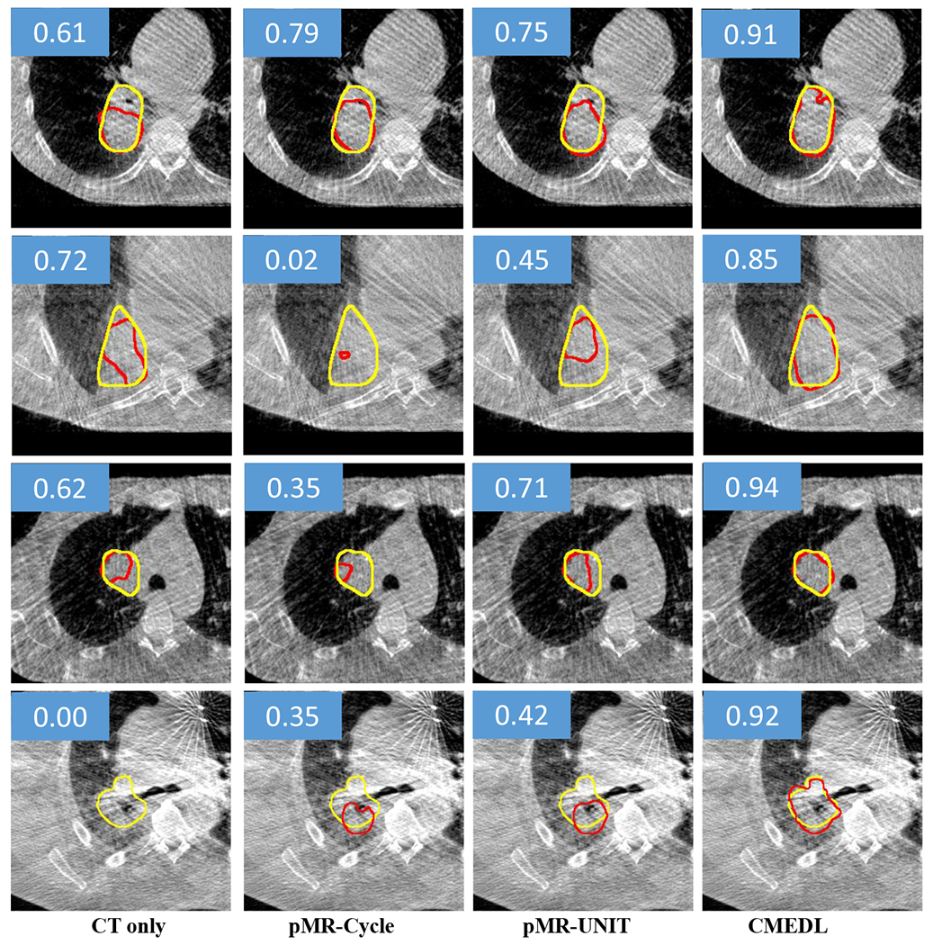
Segmentation of representative CBCT images from test set using the CMEDL approach compared with CBCT-only segmentation. Both methods used U-net as a segmentation architecture. Yellow contour indicates the manual segmentation while the red contour indicates the algorithm segmentation. The DSC score of each example is also shown in the blue rectangle area.

c. Networks training:

All networks were implemented using the Pytorch [34] library and trained end to end on Tesla V100 with 16 GB memory and a batch size of 2. The ADAM algorithm [35] with an initial learning rate of 1e-4 was used during training for the image translation networks. The segmentation networks were trained with a learning rate of 2e-4. We set λ_adv=1, λ_cyc=10, λ_CX=1, λ_hint=1 and λ_seg=5 for the coeffcient of equation 7.

A pre-trained VGG19 network using the ImageNet dataset was used to compute the contextual loss. The low level features extracted using VGG19 quantify edge and textural characteristics of images. Although such features could be more useful for quantifying the textural differences between the activation maps, the substantial memory requirement for extracting these features precluded their use in this work. Instead we used higher level features computed from layers Conv7, Conv8, and Conv9 that capture the mid- and high-level contextual information between the various organ structures. The feature sizes were 64×64×256, 64×64×256 and 32×32×512, respectively.

Due to the limited number of CBCT datasets, networks were trained using 2D image slices containing the tumor after cropping the original images (512 × 512) into 256 × 256 image patches. Image cropping was done by automatic removal of regions outside the body region through intensity thresholding, followed by hole filling, and connected components extraction to identify the largest component or body region. The networks were trained with 216 CBCT scans, validated on 20 CBCT scans stemming from 15 internal and 5 external, and tested on 38 CBCT scans stemming 33 internal and 5 external cases. Online data augmentation including horizontal flipping, scaling, rotation, and elastic deformation was used. Early stopping strategy was used to avoid over-fitting and the networks were trained up to utmost 100 epochs. In order to support reproducible research, we will make the code for our approach available with reasonable request upon acceptance for publication.

III. EXPERIMENTS AND RESULTS

Experiments were done to test the hypothesis that constraining a CBCT network to focus on certain aspects of the images during training by another network processing more informative MRI will lead to more accurate tumor volume segmentation than when using a network trained with only CBCT images. In other words, the MRI network forces the CBCT network to extract features that help it to improve segmentation performance. We tested our distillation learning framework on two different commonly used segmentation networks to assess performance differences due to network architecture. We also used a similar framework as done in [8] to assess whether UDA combined MRI network outperforms CBCT only segmentation. In the CMEDL case, the teacher network was used instead of the CBCT network for segmentation. We implemented a baseline framework using standard cycleGAN and Unet segmentor to use an implementation similar to[8], and the more advanced variational auto-encoder using the unpaired image to image translation (UNIT)[17] as the UDA network combined with Unet segmentor. All networks were trained from scratch using identical sets of training and testing datasets. Reasonable hyper-parameter optimization was done to ensure good performance by all networks.

A. Evaluation Metrics

Segmentation performance was evaluated from 3D volumetric segmentations produced by combining segmentations from 2D image patches of size 256×256. In order to establish the clinical utility of the developed method, we computed surface Dice similarity coefficient (SDSC) metric[36], which was shown to be more representative of any additional effort needed for clinical adaptation[37] than the more commonly used geometric metrics like DSC and Hausdroff distances. For completeness, we also report the DSC and Hausdroff distance metric at 95th percentile (HD95) as recommended in prior works[38]. Finally, the tumor detection rate, computed as segmentations having at least 50% overlap with the expert-segmentation reference using the DSC metric, is also reported.

The surface DSC metric emphasizes the incorrect segmentations on the boundary, as this is where the edits are most likely to be performed by clinicians for clinical acceptance. It is computed as:

$$D_{i,j}^{\left(\tau \right)}=\frac{\left|S_i\cap B_j^{\left(\tau \right)}\right|+\left|S_j\cap B_i^{\left(\tau \right)}\right|}{\left|S_i\right|+\left|S_j\right|}$$ (8)

where $B_i^{\left(\tau \right)}\subset R^3$ is a border region of the segmented surface S_i. The tolerance threshold τ = 4.38mm was computed using the standard deviation of the HD95 distances of 8 segmentations performed by two different experts blinded to each other.

a. Statistical analysis:

Statistical comparisons between the various methods was performed to assess the difference between the CMEDL vs. other approaches using paired Wilcoxon two-sided tests using the DSC accuracy measure. Adjustments for multiple comparisons were performed using Holm-Bonferroni method.

B. Tumor detection accuracy

Networks using CMEDL approach, both the distillation and CMEDL pseudo MRI (or pMRI-CMEDL) produced the most accurate tumor detection (Table I). On the other hand, both pMRI-Cycle and pMRI-UNIT methods were slightly less accurate than these two methods. The CBCT only networks were the least accurate. Segmentation accuracies are reported using tumors that were detected by at least one of all the analyzed methods. This resulted in 18 out of 20 cases for validation and 35 out of 38 cases for the testing set.

TABLE I:

Lung tumor detection rates for the various analyzed methods on validation and test sets using Unet and DenseFCN for CBCT images.

Net	Method	Validation	Test
Unet	CT only	0.85	0.72
	pMRI-Cycle	0.85	0.80
	pMRI-UNIT	0.85	0.89
	pMRI-CMEDL	0.90	0.92
	CMEDL	0.90	0.95
DenseFCN	CT only	0.80	0.69
	pMRI-Cycle	0.80	0.74
	pMRI-UNIT	0.80	0.71
	pMRI-CMEDL	0.85	0.89
	CMEDL	0.85	0.89

C. Comparison of CMEDL and CBCT only segmentations

Table. II shows the segmentation accuracies on the cross-validation (shown for completeness) and test set using the various methods for the Unet and DenseFCN segmentation architectures. As seen, both the CMEDL and pMRI-CMEDL were more accurate than CBCT only, pMRI-Cycle and pMRI-UNIT methods. The CMEDL method was significantly more accurate than the CBCT only method (P < 0.001 on Unet and P < 0.001 on DenseFCN) using DSC and (P < 0.001 for Unet and P < 0.001 for DenseFCN using SDSC metrics. Fig. 4 shows example segmentations generated on the CBCT images by using the CBCT only, pMRI-Cycle, pMRI-UNIT, and CMEDL methods using Unet network.

TABLE II:

Segmentation accuracy for CBCT dataset using the various approaches using Unet and DenseFCN networks.

Net		Validation			Test
	Method	DSC	Surface DSC	HD95 mm	DSC	Surface DSC	HD95 mm
Unet	CBCT only	0.64±0.21	0.72±0.11	16.19±11.55	0.62±0.15	0.69±0.11	21.70±16.34
	pMRI-Cycle	0.65±0.20	0.72±0.11	11.30±7.64	0.66±0.12	0.74±0.13	14.43±12.22
	pMRI-UNIT	0.66±0.19	0.71±0.10	10.55±6.98	0.66±0.11	0.76±0.13	14.56±11.80
	pMRI-CMEDL	0.74±0.18	0.80±0.09	8.87±8.98	0.69±0.10	0.79±0.11	10.42±10.58
	CMEDL	0.73±0.18	0.80±0.09	6.39±6.27	0.73±0.10	0.83±0.08	7.69±7.86
DenseFCN	CBCT only	0.63±0.18	0.59±0.12	22.88±12.91	0.58±0.14	0.66±0.15	22.15±17.19
	pMRI-Cycle	0.65±0.13	0.63±0.12	14.83±11.83	0.57±0.14	0.66±0.18	21.82±15.97
	pMRI-UNIT	0.66±0.14	0.65±0.15	20.98±15.60	0.64±0.15	0.62±0.17	25.28±15.94
	pMRI-CMEDL	0.69±0.18	0.69±0.10	17.60±9.25	0.68±0.12	0.73±0.13	14.46±11.87
	CMEDL	0.69±0.17	0.70±0.11	11.43±6.91	0.72±0.13	0.75±0.13	11.42±9.87

D. Pseudo MRI translation accuracy

We also measured the accuracy of translating the CBCT into pseudo MRI images using the CMEDL, CycleGAN and UNIT methods using Kullback-Leibler (KL) divergence measure. The CMEDL approach resulted in the most accurate translation with the lowest KL divergence of 0.082 when compared with 0.42 for CycleGAN and 0.29 for the UNIT method. Fig. 5 shows representative examples from the test set of translated pMRI images produced using the CMEDL method. As seen, tumor and various structures in the MRI are clearly visualized with clear boundary seen between tumor and central structures compared to the corresponding CBCT image.

FIG. 5:

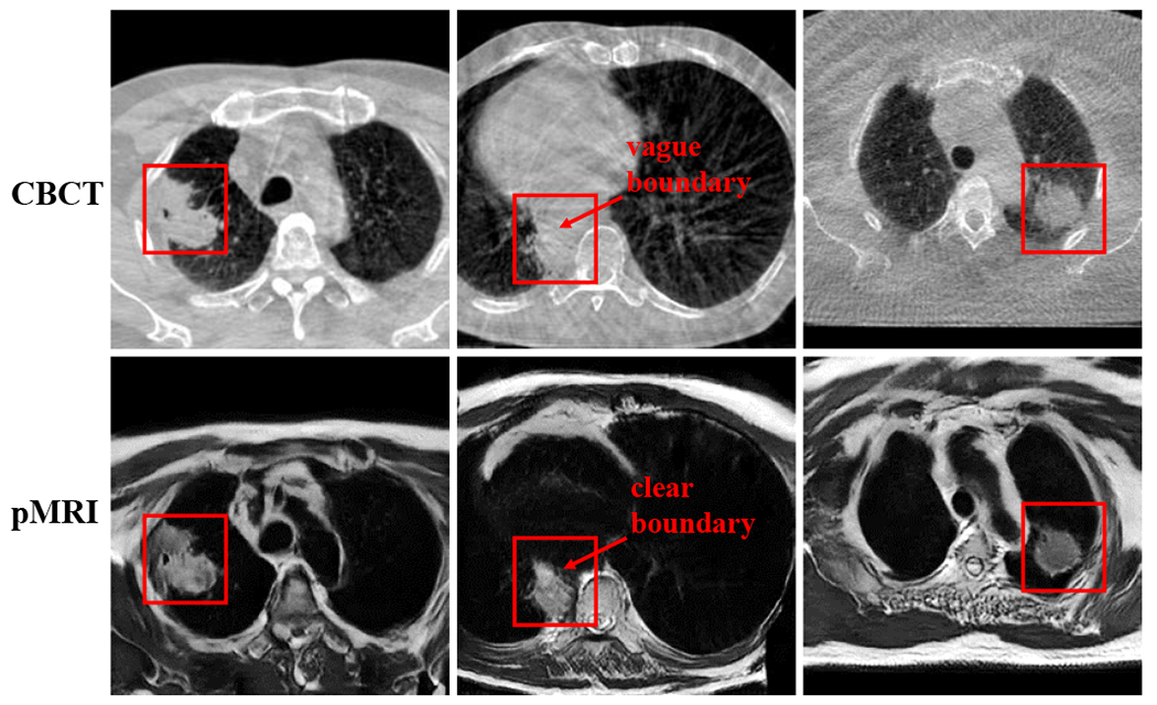
Representative examples of pMRI generated from CBCT images using the CMEDL method. The tumor region is enclosed in the red contour.

E. Visualization of feature maps produced in student network of CMEDL vs. CT only network

Finally, we studied how providing MRI information leads to differences in the computed features and ultimately segmentation improvement on CT. Fig. 6 shows example eight randomly chosen feature maps from the last layer (with size of 256×256×64) of Unet model when using the CBCT-only model (Fig. 6(a)) and the features computed from the corresponding layer of the CBCT network trained using CMEDL approach (Fig. 6(c)). For reference, the feature maps computed in the same layer for the teacher network when using the pMRI (translated from CBCT) are also shown (Fig. 6(b)). As seen, the feature maps extracted using the CBCT only method are less effective in differentiating the tumor regions from the background parenchyma when compared to the CMEDL CBCT network. Furthermore, the CBCT student network closely matches the feature maps extracted by the teacher network, albeit from a MRI-like image (or the pseudo MRI). More importantly, the CBCT student network captured the contrast inherent in the MRI between tumor and its background clearly even when it is fed only CBCT images, which in turn contributes to more accurate segmentation.

FIG. 6:

Feature activaton maps computed from (a) CBCT Unet, (b) teacher network of CMEDL, and (c) student CBCT network.

IV. DISCUSSION

In this work, we introduced a new approach to leverage higher contrast information from more informative MRI modality to improve CBCT segmentation. Our approach uses unpaired sets of MRI and CBCT images from different sets of patients and learns to extract informative features on CBCT that help to obtain a good lung tumor segmentation, even for some centrally located tumors. Our approach shows a clear improvement over CBCT only segmentation and is also slightly more accurate than using pseudo MRI representation for segmentation. More importantly, using cross-modality distillation to constrain learning improves CBCT network’s segmentation such that there is no need for a cross-modality segmentation network once the training is done. In fact, this segmentation was more slightly accurate than using the CMEDL network combined with the MR segmentation network.

To our best knowledge, this is one of the first works to address the problem of fully automatic lung tumor segmentation on CBCT images. Prior work on CBCT used semi-automated segmentation[39], and the CBCT deep learning methods were applied to segment pelvic normal organs[7, 8].

Our results showed that the MRI information educed on CBCT is most useful when used as hints through cross-modality distillation. On the other hand, the frameworks that used the synthesized pseudo MRIs directly for segmentation were less accurate. We believe this occurs due to the difficultly of producing spatially accurate translation of CBCT into pseudo MRI. This is lesser issue when using the pseudo MRI only to provide hints for high-level features extracted on CBCT, but accurate I2I translation is more important when using the translated image for segmentation. As shown, both pMRI-Cycle and pMRI-UNIT were comparable in performance. On the other hand, the pMRI-CMEDL approach, which uses side information from CBCT student network to also constrain the I2I translation improves the accuracy of the teacher network for segmenting CBCT.

Besides the lower accuracy of pMRI-CMEDL approach to CMEDL CBCT segmentation, the former method requires both the I2I translation and MRI network at testing time, ultimately increasing both the memory and computational requirements for generating CBCT segmentation. The CMEDL CBCT on the other hand is computationally simpler and only requires the CBCT segmentation network during testing.

As opposed to standard distillation methods that used a pre-trained teacher network as done in [11, 14, 40], which required paired image sets, ours is the first, to our best knowledge, that works with completely unrelated set of images from widely different imaging modalities. Removing the constraint of paired image sets makes our approach more practical for medical applications, including new image-guided cancer treatments.

As a limitation, our approach used a modest number of CBCT images for training and testing. However, to our best knowledge, this is the first approach to tackle the problem of CBCT lung tumor segmentation. Also, testing on multi-institutional datasets with different imaging acquisitions is essential to establish the generality of the developed approach and is work for future.

V. CONCLUSIONS

We introduced a novel cross-modality educed distllation learning approach for segmenting lung tumors on cone-beam CT images. Our approach uses unpaired MRI and CBCT image sets to constrain the features extracted on CBCT to improve inference and segmentation performance. Our approach implemented on two different segmentation networks showed clear performance improvements over CBCT only methods. Evaluation on much larger datasets is essential to assess potential for clinical translation.

FIG. 3:

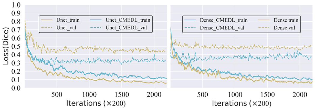
The training and validation loss for Unet and DenseFCN with and without CMEDL.

References

- [1].Seigel R, Miller K, and Jemal A, Cancer statistics, CA: A cancer journal for clinicians 70, 7–30 (2020). [DOI] [PubMed] [Google Scholar]
- [2].Bradley J, Hu C, Komaki R, Masters G, Blumenschein G, Schild S, Bogart J, Forster K, Magliocco A, Kavadi V, Narayan S, Iyengar P, Wynn RCG,R, Koprowski C, Olson M, Meng J, Paulus R, Curran W Jr, and Choy H, Long-Term Results of NRG Oncology RTOG 0617: Standard- Versus High-Dose Chemoradiotherapy With or Without Cetuximab for Unresectable Stage III NonSmall-Cell Lung Cancer, Journal of Clinical Oncology 38, 706–714 (2020). [DOI] [PMC free article] [PubMed] [Google Scholar]
- [3].Weiss E, Fatyga M, Wu Y, Dogan N, Balik S, Sleeman W, and Hugo G, Dose escalation for locally advanced lung cancer using adaptive radiation therapy with simultaneous integrated volume-adapted boost, Int J Radiat Oncol Biol Phys 86, 414–9 (2013). [DOI] [PMC free article] [PubMed] [Google Scholar]
- [4].Kavanaugh J, Hugo G, Robinson C, and Roach M, Anatomical AdaptationEarly Clinical Evidence of Benefit and Future Needs in Lung Cancer, Semin Radiat Oncol 29, 274–283 (2019). [DOI] [PubMed] [Google Scholar]
- [5].Sonke J and Belderbos J, Adaptive radiotherapy for lung cancer, Semin Radiat Oncol 20, 94–106 (2010). [DOI] [PubMed] [Google Scholar]
- [6].Sonke J, Aznar M, and Rasch C, Adaptive radiotherapy for anatomical changes, Semin Radiat Oncol 29, 245–257 (2019). [DOI] [PubMed] [Google Scholar]
- [7].Jia X, Wang S, Liang X, Balagopal A, Nguyen D, Yang M, Wang Z, Ji JX, Qian X, and Jiang S, Cone-Beam Computed Tomography (CBCT) Segmentation by Adversarial Learning Domain Adaptation, in Medical Image Computing and Computer Assisted Intervention – MICCAI 2019, edited by Shen D, Liu T, Peters TM, Staib LH, Essert C, Zhou S, Yap P-T, and Khan A, pages 567–575, Springer International Publishing, 2019. [Google Scholar]
- [8].Fu Y, Lei Y, Wang T, Tian S, Patel P, Jani A, Curran W, Liu T, and Yang X, Pelvic multi-organ segmentation on cone-beam CT for prostate adaptive radiotherapy, Med Phys . [DOI] [PMC free article] [PubMed] [Google Scholar]
- [9].Hinton G, Vinyals O, and Dean J, Distilling the knowledge in a neural network, (2015). [Google Scholar]
- [10].Bucilua C, Caruana R, and Niculescu-Mizil A, Model compression, in Proceedings of the 12th ACM SIGKDD international conference on Knowledge discovery and data mining, pages 535–541, ACM, 2006. [Google Scholar]
- [11].Romero A, Ballas N, Kahou SE, Chassang A, Gatta C, and Bengio Y, Fitnets: Hints for thin deep nets, in 3rd International Conference on Learning Representations, ICLR 2015, San Diego, CA, USA, May 7-9, 2015, Conference Track Proceedings, 2015. [Google Scholar]
- [12].Li Q, Jin S, and Yan J, Mimicking very efficient network for object detection, in Proceedings of the IEEE Conference on Computer Vision and Pattern Recognition, pages 6356–6364, 2017. [Google Scholar]
- [13].Su J-C and Maji S, Cross quality distillation, arXiv preprint arXiv:1604.00433 3 (2016). [Google Scholar]
- [14].Gupta S, Hoffman J, and Malik J, Cross modal distillation for supervision transfer, in Proceedings of the IEEE conference on computer vision and pattern recognition, pages 2827–2836, 2016. [Google Scholar]
- [15].Jiang J, Hu Y, Liu C, Halpenny D, Hellmann MD, Deasy JO, Mageras G, and Veeraraghavan H, Multiple Resolution Residually Connected Feature Streams for Automatic Lung Tumor Segmentation From CT Images, IEEE Transactions on Medical Imaging 38, 134–144 (2019). [DOI] [PMC free article] [PubMed] [Google Scholar]
- [16].Zhu J-Y, Park T, Isola P, and Efros A, Unpaired image-to-image translation using cycle-consistent adversarial networks, in Intl. Conf. Computer Vision (ICCV), pages 2223–2232, 2017. [Google Scholar]
- [17].Li Y, Fang C, Yang J, Wang Z, Lu X, and Yang M-H, Universal style transfer via feature transforms, in Advances in Neural Information Processing Systems, pages 386–396, 2017. [Google Scholar]
- [18].Hugo GD, Weiss E, Sleeman WC, Balik S, Keall PJ, Lu J, and Williamson JF, A longitudinal four-dimensional computed tomography and cone beam computed tomography dataset for image-guided radiation therapy research in lung cancer, Medical Physics 44, 762771 (2017). [DOI] [PMC free article] [PubMed] [Google Scholar]
- [19].Tustison N and Avants B, Explicit B-spline regularization in diffeomorphic image registration, Front Neuroinform 7 (2013). [DOI] [PMC free article] [PubMed] [Google Scholar]
- [20].Alam S, Thor M, Rimner A, Tyagi N, Zhang S-Y, Kuo L, Nadeem S, Lu W, Hu Y-C, Yorke E, and Zhang P, Quantification of accumulated dose and associated anatomical changes of esophagus using weekly magnetic resonance imaging acquired during radiotherapy of locally advanced lung cancer, Phys Imaging Radiat Oncol 13, 36–43 (2020). [DOI] [PMC free article] [PubMed] [Google Scholar]
- [21].Goodfellow I, Pouget-Abadie J, Mirza M, Xu B, Warde-Farley D, Ozair S, Courville A, and Bengio Y, Generative adversarial nets, in Advances in Neural Information Processing Systems (NIPS), pages 2672–2680, 2014. [Google Scholar]
- [22].Jiang J, Hu Y-C, Tyagi N, Zhang P, Rimner A, Mageras GS, Deasy JO, and Veeraraghavan H, Tumor-Aware, Adversarial Domain Adaptation from CT to MRI for Lung Cancer Segmentation, in International Conference on Medical Image Computing and Computer-Assisted Intervention, pages 777–785, Springer, 2018. [DOI] [PMC free article] [PubMed] [Google Scholar]
- [23].Mechrez R, Talmi I, and Zelnik-Manor L, The contextual loss for image transformation with non-aligned data, arXiv preprint arXiv:1803.02077 (2018). [Google Scholar]
- [24].Simonyan K and Zisserman A, Very deep convolutional networks for large-scale image recognition, arXiv preprint arXiv:1409.1556 (2014). [Google Scholar]
- [25].Lin G, Milan A, Shen C, and Reid I, Refinenet: Multi-path refinement networks for high-resolution semantic segmentation, in Proceedings of the IEEE conference on computer vision and pattern recognition, pages 1925–1934, 2017. [Google Scholar]
- [26].Radford A, Metz L, and Chintala S, Unsupervised representation learning with deep convolutional generative adversarial networks, arXiv preprint arXiv:1511.06434 (2015). [Google Scholar]
- [27].He K, Zhang X, Ren S, and Sun J, Deep Residual Learning for Image Recognition, arXiv preprint arXiv:1512.03385 (2015). [Google Scholar]
- [28].Ulyanov D, Vedaldi A, and Lempitsky V, Improved texture networks: Maximizing quality and diversity in feed-forward stylization and texture synthesis, in Proceedings of the IEEE Conference on Computer Vision and Pattern Recognition, pages 6924–6932, 2017. [Google Scholar]
- [29].Ronneberger O, Fischer P, and Brox T, U-net: Convolutional networks for biomedical image segmentation, in International Conference on Medical Image Computing and Computer-Assisted Intervention (MICCAI), pages 234–241, Springer, 2015. [Google Scholar]
- [30].Jégou S, Drozdzal M, Vazquez D, Romero A, and Bengio Y, The one hundred layers tiramisu: Fully convolutional densenets for semantic segmentation, in Computer Vision and Pattern Recognition Workshops (CVPRW), 2017 IEEE Conference on, pages 1175–1183, IEEE, 2017. [Google Scholar]
- [31].Isola P, Zhu J-Y, Zhou T, and Efros AA, Image-to-image translation with conditional adversarial networks, arXiv preprint (2017). [Google Scholar]
- [32].Ioffe S and Szegedy C, Batch normalization: Accelerating deep network training by reducing internal covariate shift, arXiv preprint arXiv:1502.03167 (2015). [Google Scholar]
- [33].Huang G, Liu Z, Van Der Maaten L, and Weinberger KQ, Densely connected convolutional networks, in Proceedings of the IEEE conference on computer vision and pattern recognition, pages 4700–4708, 2017. [Google Scholar]
- [34].Paszke A, Gross S, Chintala S, Chanan G, Yang E, DeVito Z, Lin Z, Desmaison A, Antiga L, and Lerer A, Automatic differentiation in PyTorch, (2017). [Google Scholar]
- [35].Kingma D-P and Ba J, Adam: A method for stochastic optimization, Proceedings of the 3rd International Conference on Learning Representations (ICLR) (2014). [Google Scholar]
- [36].Nikolov S et al. , Deep learning to achieve clinically applicable segmentation of head and neck anatomy for radiotherapy, arXiv preprint arXiv:1809.04430 (2018). [Google Scholar]
- [37].Vaassen F, Hazelaar C, Vaniqui A, Gooding M, van der Heyden B, Canters R, and van Elmpt W, Evaluation of measures for assessing time-saving of automatic organ-at-risk segmentation in radiotherapy, Physics and Imaging in Radiation Oncology 13, 1 – 6 (2020). [DOI] [PMC free article] [PubMed] [Google Scholar]
- [38].Menze BH et al. , The multimodal brain tumor image segmentation benchmark (BRATS), IEEE transactions on medical imaging 34, 1993 (2015). [DOI] [PMC free article] [PubMed] [Google Scholar]
- [39].Veduruparthi BK, Mukhopadhyay J, Das PP, Saha M, Prasath S, Ray S, Shrimali RK, and Chatterjee S, Segmentation of Lung Tumor in Cone Beam CT Images Based on Level-Sets, in 2018 25th IEEE International Conference on Image Processing (ICIP), pages 1398–1402, 2018. [Google Scholar]
- [40].Chen G, Choi W, Yu X, Han T, and Chandraker M, Learning efficient object detection models with knowledge distillation, in Advances in Neural Information Processing Systems, pages 742–751, 2017. [Google Scholar]
- [41].layers are only counted on layers that have tunable weights