

Abstract
Stereoscopic depth has a mixed record as a guiding attribute in visual attention. Visual search can be efficient if the target lies at a unique depth; whereas automatic segmentation of search arrays into different depth planes does not appear to be pre-attentive. These prior findings describe bottom-up, stimulus-driven depth guidance. Here, we ask about the top-down selection of depth information. To assess the ability to direct attention to specific depth planes, Experiment 1 used the centroid judgment paradigm which permits quantitative measures of selective processing of items of different depths or colors. Experiment 1 showed that a subset of observers could deploy specific attention filters for each of eight depth planes, suggesting that at least some observers can direct attention to a specific depth plane quite precisely. Experiment 2 used eight depth planes in a visual search experiment. Observers were encouraged to guide their attention to far or near depth planes with an informative but imperfect cue. The benefits of this probabilistic cue were small. However, this may not be a specific problem with guidance by stereoscopic depth. Equivalently poor results were obtained with color. To check and prove that depth guidance in search is possible, Experiment 3 presented items in only two depth planes. In this case, information about the target depth plane allows observers to search more efficiently, replicating earlier work. We conclude that top-down guidance by stereoscopic depth is possible but that it is hard to apply the full range of our stereoscopic ability in search.
Keywords: Visual attention, Visual search, Depth, Stereoscopic disparity, Centroid estimation
Horizontal disparities between the two eyes’ retinal images are the primary cue for stereoscopic depth (Duan et al., 2021; Wheatstone, 1838). Considering the three-dimensional world we live in, intuition might suggest that depth information would be beneficial in the visual search tasks of everyday life. However, stereoscopic depth has a mixed record as a “guiding attribute” in visual attention (Wolfe & Horowitz, 2017). Some previous studies do suggest that bottom-up, stimulus-driven depth information can play a guiding role in search. For example, Nakayama and Silverman (1986) found that when the target has a unique depth and all distractors are located at another depth, the search time is independent of the number of distractors. They concluded that the depth information can be processed at a pre-attentive stage. A follow-up study by de la Rosa et al., (2008) investigated the minimum disparity required for efficient depth X color conjunction search. They found that efficient search occured with disparities of 6 arcmins or more. McSorley and Findlay (2001) examined the eye movement patterns of a search task using targets defined either by a depth or a color singleton. Search for either of these feature targets was found to be quite efficient with approximately 70% of first saccades landing on the target. Plewan and Rinkenauer (2018a) found that “surprising” depth information captured attention. In real-world search tasks, Godwin et al., (2017) found adding depth to the items improved accuracy for the transparent stimuli. Participants learned to search more exhaustively in displays containing depth (Godwin et al., 2020). Besides visual search tasks, Sarno et al., (2019) found a benefit of depth information in a change-detection paradigm, and that the benefits were observed when the working memory load exceeded max capacity. Ogawa and Macaluso (2015) also found more accurate and faster detections for foreground changes and overall better performance in binocular than monocular conditions with a flicker paradigm. Caziot and Backus (2015) assessed the effect of disparity on object recognition by giving an object a brief stereoscopic offset and found the object was easier to recognize. They concluded that binocular vision confers an advantage for recognizing objects. The above studies all found stereoscopic depth information to be a useful cue that improved task performance.
On the contrary, there are studies showing that although visual search is faster and more accurate with depth knowledge (Reis et al., 2011), there is no evidence of improved search efficiency as indexed by the slope of the reaction time (RT) × Set Size function (Roberts et al., 2015). This suggests that the benefits of stereoscopic depth might occur in early vision (e.g. in image segmentation) or at a decision stage, rather than having an impact on search. O’Toole and Walker (1997) examined the generality of the claim that stereoscopic disparity is detectable in parallel using random-dot stereograms, and they found none of their RT × set size search slopes fit the classically flat pattern which is associated with parallel access of a basic feature. Finlayson et al., (2013) asked whether attending to one depth plane would improve search efficiency by eliminating interference from distractors on the other depth plane. No differences were found between one-depth and two-depth with a conjunction search task, despite prior knowledge of the depth plane containing the target. The parallel search of Nakayama and Silverman (1986) may be achieved by detecting a depth singleton rather than by restricting search to a single depth plane.
To what extent does direct attention to a particular plane in depth enable observers to filter out interference from another depth plane? Theeuwes et al., (1998) found that observers cannot prevent attention capture from distractors in another depth plane. Plewan and Rinkenauer (2021) further investigated this issue with a multiple target search task. Based on their results, they concluded that depth is an important but easily perturbed feature guiding attention. Depth guidance may exist but may be an error-prone process or interfered with by other features (Plewan & Rinkenauer, 2020).
The existing studies indicate that there is some guiding role for bottom-up, stimulus-driven depth information. There is relatively little research on the top-down attentional control by stereoscopic depth and most of that work is qualitative in nature. In order to further investigate the extent to which observers can deploy their attention to different depth spaces while eliminating the interference from non-target depths, this paper seeks to quantitatively measure the top-down ability to direct visual attention to specific depth regions using a relatively recent experimental paradigm called “centroid estimation” (Sun et al., 2016a).
With the centroid paradigm, we can quantitatively measure the attentional control of depth information, and obtain selectivity weights for the target depth plane and for each irrelevant depth plane during attention deployment. These weights constitute a portrait of an attention filter for stereoscopic depth information similar to the filters that Sun et al. (2016a) derived for color. Such filters describe the effectiveness of the human visual system in controlling attention on the basis of a specific feature.
In Experiment 1, we quantitatively measured the ability to selectively process different depths using the centroid estimation paradigm. We found that a subset of observers who passed the screening for temporal stereoscopic ability could deploy specific attention filters for each of eight depth planes, suggesting that at least some observers can direct attention to a specific depth plane quite precisely. Having the ability to attend in depth is not the same as being able to use that ability to guide attention in visual search. In Experiment 2, we explored the question of depth guidance in visual search using similar multi-depth plane stimuli. The results showed small benefits of depth cues, similar to what we find in a color cue condition. While some observers can direct attention to specific depth planes, it seems to be difficult to deploy this skill effectively in search. In the face of that largely negative finding, we sought to confirm that some guidance by stereo depth information is possible. Experiment 3 presented items in only two disparity-defined depth planes. In this case, information about the target depth plane allowed observers to search more efficiently in a two-depth condition, compared to a one-depth condition.
Experiment 1 –. Selective processing of stereoscopic depth
This experiment studies visual selective attention for depth. When the target depth is known, can human observers selectively process the information at the target depth using top-down control of attention while not being distracted by irrelevant information in non-target depth planes?
The schematic diagram of the centroid experiment is shown in Figure 1. During the experiment, a cloud of dots stimuli was briefly presented to the observers. Three dots on the target plane were the target dots, and all dots on the other depth planes were distractors. Observers were instructed to estimate the center of gravity, based only on the three target dots while attempting to ignore the distractor dots. Based on the position of all dots and the estimated centroid given by the observers, the weight of target depth and the interference from non-target depth could be measured quantitatively with a regression model.
Figure 1.

The centroid paradigm: exemplar procedure and analysis
Depth planes were generated with stereoscopic disparity. There were three dots assigned to each depth plane. If the observers could correctly select the target depth and completely ignore interferences from other depths, the estimated centroid should be the center of gravity of the three target dots with some random response errors added. However, any of the other dots might have some impact on the centroid judgment if the observers cannot perfectly select the target depth and ignore the interference. The weights of different depths in this top-down attentional control process define the attention filters for the target depth plane. Using the method of Sun et al (2016a,b), the sensitivity function can be regressed by analyzing the contribution of each depth plane to the centroid estimation (detailed in the Appendix ‘Estimation of Attention Filter Weight’).
Participants
Informed consent was obtained from all participants under procedures approved by the IRB of Brigham and Women’s Hospital. All observers had normal or corrected-to-normal vision and were unaware of the research goal of the experiments. Stereoacuity was measured using the Titmus Stereo test (Stereo Optical Co., Chicago, IL). Since our centroid task requires good stereopsis using brief stimulus presentations, we performed a quite rigorous screening for temporal stereoscopic ability (detailed in ‘Screening for Temporal Stereopsis’ section, below). All participants were young adults (18–30 yrs old). Precise age details were lost, unfortunately. Only five out of 17 participants passed the screening test. These five proceeded with the formal experiment. Because of this high exclusion rate, we would not want to conclude that our results show that ‘average’ participants have the stereoscopic filtering abilities that we demonstrate here. Rather, these data should be considered to be an existence proof that some observers, who come into the experiment with good stereoscopic abilities, can perform this filtering.
Apparatus and Stimuli
Stimuli consisted of left eye images and right eye images that were drawn and presented using MATLAB with the Psychophysics Toolbox (Brainard, 1997) and presented on two 20” Planar PL2010M LCD (Planar Systems Inc.) monitors respectively with a resolution of 1600x1200 pixels, and a 60Hz refresh rate. Participants were seated approximately 70cm from the screen. The two monitors were mounted one above the other with a polarized mirror set in between. Stereoscopic perception was achieved when observers wore polarized glasses.
The experimental stimulus was displayed in the center of the screen within a 512 × 512-pixel area (visual angle 10.8°). The stereoscopic disparity of the depth planes ranged from – 56 arcmins to 56 arcmins, and the disparity difference between adjacent depth planes was 16 arcmins. The experimental stimuli were square dots, 12 pixels on a side. The visual angle subtended was 0.25°. To avoid conditions where the centroid of three target dots was close to the centroid of distractor dots, the locations of all target dots and distractor dots were taken from two bivariate Gaussian distributions with different mean but the same standard deviation (2.5°), and the two mean values are independently drawn from a circular, bivariate Gaussian distribution with μ=0, σ=0.53°. The independent random selection of the two mean values improves the statistical efficiency in the centroid estimation (Sun et al., 2016a). To prevent any two dots from overlapping and to avoid false matches during binocular fusion, as the stimulus was being generated, each new dot was required to be no closer to any previously placed dot than minAllowDist pixels, where minAllowDist is the sum of the maximum parallax distance (45 pixels), and twice the dot-width (24 pixels).
Procedure and design
The experimental procedure is shown in Figure 3. The task was to estimate the centroid of target dots among distractor dots by mouse-click as accurately as possible. Before stimulus onset, observers were provided with the target depth plane (rectangular frame). Next, all stimuli dots appeared for a short time (Stimulus Onset Asynchrony, SOA = 300msec, only the target dots are shown in the figure for illustration purposes), and then all dots disappeared. The SOA of the test stimulus is considered brief enough to largely preclude volitional eye movements (Sun et al., 2016b). Observers estimated the centroid of the three dots within the target depth plane. Target depth remained fixed throughout a block. Feedback was provided after each trial. It included the stimulus, target centroid, observer’s response, and estimation error. The error was calculated as the Euclidean distance between the estimated centroid and the actual target centroid in pixels.
Figure 3.

Cartoon of the experimental procedure: (a) Fixation frame, 1s. (b) Stimulus, 300 ms. (c) Response display shown until a response is made. (d) Feedback display that shows the stimulus, the target centroid, the observer’s response, and the error.
Preliminary experiments found that some observers could not process the stereo information in 300 msec (Richards, 1971). Obviously, the study is not interesting if observers cannot perceive the stereo layout. Although the temporal resolution of the stereoscopic vision is poor compared with luminance (Caziot et al., 2015), similar to luminance contrast perception, the human visual system can extract stereo information from transient visual stimuli within about 50 ms (Breitmeyer et al., 2006; White & Odom, 1985), vergence eye movements can be generated within just 80 ms in response to a disparity step (Busettini et al., 2001) and long-term training enabled some experts to distinguish eight depth planes in parallel (Reeves & Lynch, 2017). However, there are still many individuals who are not able to reliably experience stereopsis in brief stimuli for various reasons (Richards, 1970) and static tests like the Titmus stereoscopic test chart cannot measure the temporal characteristics of stereopsis. Accordingly, we added a temporal screening test.
Screening for Temporal Stereopsis
An exemplar stimulus for our temporal stereopsis screening is shown in Figure 4. The only difference from the centroid estimation experiment is that three target dots are red and the other dots are black. The other 21 black dots were presented across the other 7 depths with 3 lying at each depth for the coplanar condition. In the non-coplanar case, one red dot had a different disparity from the other two so that they would define a plane, rotated out of the frontal plane. The experimental task was to judge whether the three red dots were at the same depth. Observers responded using cursor keys. Because color is a basic visual feature, we assumed that the three red dots could be selected using minimal attentional resources. Thus, the factor determining the time required to judge whether they are coplanar can be used as an estimate of the observer’s temporal stereoscopic sensitivity, at least, for our screening purposes.
Figure 4.

Screening test of temporal stereopsis: Judge whether three red dots are coplanar. You can cross fuse to see stereo. This is an example of a non-coplanar case.
In the experiment, the time threshold required for observers to perceive stereoscopic depth was measured using a 1-up/3-down staircase method. The initial presentation time of the experiment was 1500ms. If the observers answered correctly three times in a row, the stimulus presentation time decreased by 50ms (3-down). If they continued to answer correctly, the time continued to decrease. When the observers answered incorrectly, the presentation time increased by 50ms (1-up), otherwise, the stimulus presentation time remained unchanged. A total of 64 trials were conducted, and the mean of the last 6 reversals in presentation time was taken as the threshold. Such a staircase estimates the 79.4% point on the accuracy × stimulus duration psychometric function (Levitt, 1971). Figure 5 shows examples of temporal screening for two observers. The passing criterion was set at 500ms. The yellow and purple asterisks in the figure represent the last six reverses of the two observers. In this example, the observer in red passed the test with a threshold of 417 milliseconds, but the observer in blue failed with a threshold of 1400 milliseconds.
Figure 5.

Examples of temporal screening for two observers. Data from two 1-Up/3-Down staircase measurements of the threshold for detecting if three dots lie at the same depth. The last six reversals are marked with yellow (failed) and purple (passed) asterisks and are averaged to obtain the threshold.
The observers who passed the temporal stereopsis screening proceeded to the main experiment. In the main experiment, there was a training session, intended to reduce the noise in individuals’ performance in the centroid judgment. Observers were trained to judge the centroid of different numbers of dots in different depth planes with a total of 8 (depth) × 5 (dots number: 1, 3, 6, 12, 24) × 20 trials = 160 training trials. For each training trial, the true centroid was provided as feedback. Furthermore, 300 additional practice trials were performed to ensure observers’ performance was relatively stable and was no longer improving. During this practice session, only stimuli in which the target depth was the nearest depth plane were displayed and the number of dots was always 24.
The formal experiment was divided into 16 blocks with 60 trials in each block, and the target depth in each block remained unchanged. The target depth between blocks gradually increased from the nearest plane (1) in front of the screen to the farthest depth plane (8) behind the screen, and then returned in reverse order to avoid an order effect. The whole experiment included 64 (screen) + 160 (train) + 300 (practice) + 960 (test) = 1484 trials in total, which took about 2.5 hours. Coordinates and depth information of all dots in each trial and the estimated centroid location were recorded.
Results & Discussions
A total of five observers passed the stereoscopic test and completed all experiment sessions. Figure 6 shows average values for “Data-drivenness” and “Efficiency” for each depth. These metrics were taken from Sun et al (2016b). Data-drivenness reflects the proportion of the results determined by the stimulus as opposed to some default location to which the Os’ response is assumed to tend. Efficiency estimates the lower bound on the proportion of dots in the display that the subject included in their centroid computation. Error bars show the standard error of the mean (SEM). It can be seen that the Data-drivenness at different depths is high (mean 0.7623), indicating that the centroid was mainly determined by the displayed stimuli. The mean of Efficiency is 0.6652 which implies that, on average, an observer was including at least two-thirds of all the dots in the stimulus display for the centroid computation.
Figure 6.

(a) Data-drivenness and (b) Efficiency from attention filter estimation (methods taken from Sun et al. (2016)). Error bars indicate ±1 SEM.
The estimated attention filters for depth are shown in Figure 7, where (a) - (e) are attention filter selectivity of 5 observers respectively, and (f) is the mean filter selectivity. The details of the analysis method for driving these filters are given in the Appendix. Taking (a) as an example, the light blue line on the left indicates the contribution of each depth plane to the centroid estimation when the target depth plane was 1 (the nearest depth plane to the observer). In (a), the weight of depth #1 was very high (≈ 0.86), indicating that the dots in target depth 1 had a large weight on the centroid estimation, while the weights of other dots were small (all less than 0.05), which means that the distractor dots on non-target depth have little impact. Observer 1’s attentional selectivity for all depths was quite accurate. They could allocate visual attention almost perfectly to the target depth and ignore interference from other depths. Similarly, observer 2’s selectivity to different depths was also relatively accurate with an average target depth weight of 0.72. Observer 3 performed differently. When the target depth was 1, 5, and 8, the selectivity was high, but for depths 2 and 7, the selectivity was poor. Taking depth 2 as an example (red line in Figure (7c)), while the weight of target depth 2 (0.41) was the largest, the weights of depths 1 and 3 on the depth 2 centroid were not much smaller (0.30 and 0.12). This indicates that observer 3 could not narrow their depth focus to just depth #2. The estimation results of attention filters for other observers can also be interpreted similarly.
Figure 7.

Estimated attention filters for depth. Lines with different colors represent filter weights of different target depths, as shown in the legend. (a-e) filter weights estimation for observers 1–5, and (f) the average. Error bars indicate 95% confidence intervals.
The centroid estimation error in visual angle under different target depths is shown in Figure 8. Figure 9 shows the correlation between filter weight for the correct depth plane and error in the centroid task. The strong negative correlation (p < .001, R2 = .6205) can be taken as a sanity check for the method. The higher the weight on the target depth, the more accurate the centroid estimation.
Figure 8.

Errors in centroid estimation for different target depths. Error bars indicate ±1 SEM.
Figure 9.

Regression analysis between filter weights and estimation errors
These results showed that at least some human observers can selectively attend to specific depth planes with high selectivity, and the selectivities for depth are comparable for different stereoscopic depths. The weights of the nearest target depth (1) and the furthest target depth (8) are higher than other depths because the depth planes in the middle were subject to interference from depth from both sides, while the nearest and furthest depth planes are only subject to interference from one side. Although this tendency appeared visible in the mean attention filter, it was not statistically reliable. One-way ANOVA showed no main effect of target depth on filter weights (F(7, 32) = 1.55, p= .19), and post hoc Tukey tests showed no significant differences among the weight of each depth (all ps > .30).
Experiment 2 –. Visual search in multi-depth with probabilistic cue
Experiment 1 showed that observers who passed the screening test could selectively pay attention to a certain depth and ignore interference from other depths, and perform spatial segmentation according to the depth information. Given that finding, Experiment 2 moved on to study whether the visual system can use this selectivity in the service of another task. Specifically, can observers search visual space from front to back or from back to front? Visual search is a ubiquitous task in daily life. An ability to guide attention in depth during search would seem to be a useful skill. To assess this possibility, we designed a multi-depth visual search task based on probabilistic cues that encouraged observers to search from front to back (or from back to front, depending on the cue).
Previous visual search in depth experiments only involved three depth planes at most (Dent et al., 2012; Finlayson et al., 2013), and most of the cues provided were only divided into effective and ineffective cases. In experiment 2, we introduced a visual search in multi-depth task based on probabilistic cues, which is a novel experimental paradigm for visual search in depth space. Figure 10a shows a schematic diagram of the experiment. The stimuli were again composed of 8 depth planes. The task was to search for the target number “2” among distracting items number 5s. Drawn in a ‘digital’ font, the 2 and 5 are mirror images of each other, and search for a 2 among 5s is known to be inefficient (e.g Wolfe, 2010).
Figure 10.
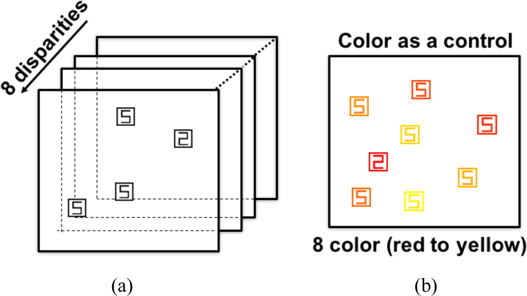
(a) Configuration in multi-depth experiment (b) Multi-color as a control
Apparatus and Stimuli
The experimental apparatus were the same as those in experiment 1. Stimuli fell within a region subtending 20° ×20° visual angle, the size of each stimulus was 50 × 50 pixels (visual angle 1.06°), the stereoscopic disparity range of the depth plane was from −21 arcmins to 21 arcmins and the disparity difference between adjacent depth planes was 6 arcmin. All stimuli were distributed in a 6 × 6 grid array. To avoid overlapping with the fixation cross located in the center of the screen, the middle four positions of the grid array were left blank. All stimuli appeared randomly in the remaining 32 grid locations with random jitter to avoid confounds that may be introduced by regular arrangement. The number of items in the search array (= the set size) had three levels (8, 16, 24). A previous study pointed out that previous failures to observe depth guidance may have been attributable to insufficient time for the resolution of depth (Marrara & Moore, 2000). To ensure that the observers had enough time to resolve stereo vision, placeholders with the shape of a digital 8 were presented at all potential locations for 1500 milliseconds before the presentation of the experimental stimuli to help the observers form a stereo impression. After 1500 ms, some placeholders changed to target number 2 or distractor item number 5 accordingly. Other placeholders disappeared leaving only 8, 16, or 24 items on the screen. Targets were present on 50% of trials. Observers were asked to respond as quickly and accurately as possible with one key for target present and another for target absent responses.
As noted, an unguided search for a 2 among 5s would be inefficient. It can be made more efficient by giving a hint as to where the 2 might be located. In the depth version of Experiment 2 (Figure 10a), we provided depth cues. In a color control condition, shown in Figure 10b, we provided color cues in the place of depth cues. The range of the colors in RGB coordinates varied from red (255 0 0) to yellow (255 255 0) in steps of 36 units on the green channel. In HSV coordinates, colors varied from [0.0000, 1.0000, 1.0000 ] to [0.1667,1.0000,1.0000 ] in hue steps of about 0.024. As shown in Figure 11, there were four depth conditions. Participants could be informed that the target would be most likely in the near, middle, or far depth planes or that all planes were equally probably. In color, only two conditions were used. Participants could be informed that the target would be most likely in the redder hues or they were informed that color was irrelevant.
Figure 11.
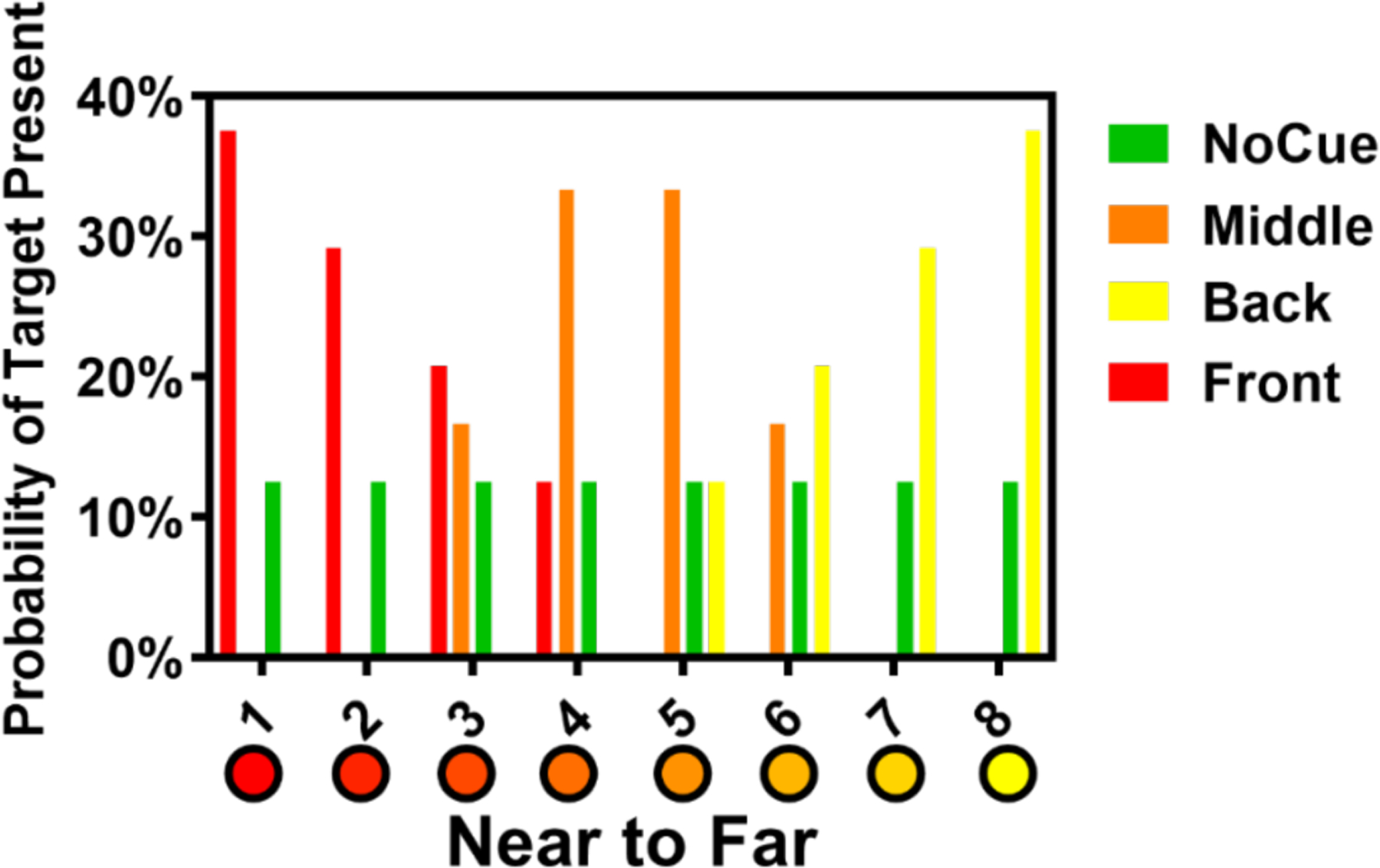
Probabilistic cues. (Multi-depth: 1 for near, 8 for far. Multi-color: 1 for red, 8 for yellow.)
Simulation of probabilistic cues
The slope of the RT × set size function should be shallower if observers guided their attention on the basis of the depth cues. To quantify the prediction, we simulated the visual search process based on the probability distribution of targets. That is, if observers are cued to the near distances, RTs should be shortest if the target is in the front, and so forth. Results are shown in Figure 12. When the location of the target was uncued, observers would need to examine an average of (n+1)/2 items, if we model search as serial, sampling without replacement. If observers could use the cue, the slope would drop to about 40% of the random slope. The relative reduction is essentially the same if we assume sampling with replacement (Horowitz & Wolfe, 1998, 2005). Since we had cued and uncued conditions, the important point was that effective use of the cues should markedly reduce the slope of the RT × set size condition, relative to the No-Cue condition.
Figure 12.

Simulation on effects of probabilistic cues. Simulated slopes of functions are given next to condition names.
Participants
Fourteen observers (mean age = 28.9 years, SD = 7.1, eight females) participated in this experiment. All had normal or corrected-to-normal vision and were unaware of the research goal of the experiments. Stereoacuity was measured using the Titmus Stereo test (Stereo Optical Co., Chicago, IL). We did not test for temporal abilities because observers always had 1500 msec to establish stereoscopic depth on each trial.
Procedure
The multi-depth experiment was divided into four blocks according to cue conditions: no cue, cue near, far, or middle, and the multi-color was divided into two blocks: no cue and cue red. The cues were changed between blocks of trials. Each block included 18 training and 144 testing trials. The set size and target presence were all randomly assigned in each block, and the experimental order of each block was balanced among observers. Color control conditions were mixed colors with and without a cue to bias attention to red. The experimental order of multi-depth experiment and multi-color control was also counter-balanced.
Results & Discussions
The data of participants whose average error rate was more than 20% were excluded from further analysis, leaving a total of twelve participants. The average error rate was 3.85%, and all error trials were eliminated in the subsequent analysis. In addition, trials with RTs less than 200ms or larger than 5000ms were excluded as outliers (1.86%). A two-way ANOVA on arcsine transformed error rates revealed no significant difference between multi-depth and multi-color experiment (F(1, 66) = 1.61, p = .21), no significant effect of cue type (F(3, 66) = 0.21, p = .891), as well as no significant interaction between different experiments and cue type (F(1, 66) = 0.075, p = .79).
RT × set size functions are shown in Figure 13. The figure indicates that RTs were somewhat shorter for cue front and cue back conditions. However, while a two-way (cue type × set size) repeated-measures ANOVA conducted on target-present RTs of multi-depth search revealed main effect of set size (F(2, 22) = 44.55, p < .001), there was no effect of cue type (F(2.10, 23.04) = 2.45, p = .11) and no interaction between cue and set size (F(2.94, 32.38) = 0.80, p = .50). For violations of sphericity in repeated-measures ANOVA, p-values were adjusted with the Greenhouse-Geisser correction (Greenhouse & Geisser, 1959). The results showed that RTs increased significantly with the increase of set size, and RTs between cue types were not significantly different. The insignificant interaction effect indicated that the search slopes between cue types were not significantly different. Furthermore, the paired sample t-test of search slopes showed that the front, back, and middle cues did not significantly improve the search efficiency (all t(11) < 1.96, all ps > .076). Similarly, the repeated-measures ANOVA of target-absent RTs showed a main effect of set size (F(2, 22) = 52.85, p < .001), but no effect of cue type (F(2.10, 23.12) = 2.97, p = .069) and no interaction between cue and set size (F(3.25, 35.77) = 1.79, p = .16). The marginal p-values for the effects of cues suggested that a weak, if significant effect might be found by a more powerful experiment. However, any effect looks much smaller than the predicted effect shown in Figure 12.
Figure 13.

Results of Experiment 2: RT × set size functions for multi-depth and multi-color conditions. Slopes of functions are given parenthetical next to condition names. Error bars indicate ±1 SEM.
Interestingly, the benefits of a color cue were also more modest than might have been expected. For the color control condition, the repeated-measures ANOVA of target-present RTs of the multi-color search experiment revealed main effects of set size (F(2, 22) = 40.82, p< .001). Here, the main effect of cue type was significant, if unimpressive (F(1, 11) = 5.15, p = .044), but the interaction effect between them was not significant (F(1.65, 18.10) = 0.28, p = .72). The introduction of the color cue reduced the RTs in the target-present trials but it did not reduce RT × set size slopes. A paired t-test result of search slopes between color cue and no cue was insignificant. The repeated-measures ANOVA of target-absent RTs revealed main effect of set size (F(2, 22) = 63.22, p < .001), but no effect of cue type (F(1, 11) = 1.12, p = .31) and no interaction between cue and set size (F(1.67, 18.36) = 2.43, p = .12).
It can be seen from the above statistical analysis that the multi-depth search task found no improvement of cues on search efficiency, which was inconsistent with the simulation results. One possible reason was that in experiment 1, only a few of the initially screened observers had accurate selectivity for depth. Perhaps only those observers with accurate depth selectivity can guide attention from front to back or vice versa. Therefore, the five observers in experiment 1 were brought back to participate in this multi-depth (color) experiment. All other aspects of the experimental designs, apparatus, and procedures remained unchanged. After excluding error trials and abnormal RTs, these five observers showed the same main effect for the color cue, but, like the other observers, no other reliable cue effects were found (all t(4) < 1.59, all ps > .18).
If all 17 observers of Experiment 2 were pooled together for a further analysis, the repeated-measures ANOVA on target-present RTs, of course, revealed the main effect of set size (F(2,32) = 62.80, p < .001). Now, there was a significant effect of cue type (F(2.21, 35.36) = 3.81, p = .028). This suggested that near and far cues do produce reduced RTs, though this analysis was post hoc. In any case, the effect was weak (compare Figure 12 with Figure 1S in the supplementary material). There were still no interaction effects, indicating that there was still no reliable improvement in search efficiency.
Figure 14 shows slopes for depth cued conditions plotted against uncued conditions of multi-depth experiment. There are three points for each observer representing three conditions of cue Front, Back, or Middle. It can be seen that no observer was able to use probabilistic cues perfectly with data lying on or below the 5:2 line predicted by the simulation shown in Figure 12. Some observers produced cued slopes that fall below the 1:1 line, suggesting an improvement in efficiency. Other observers produced slopes that lie above the 1:1 line. If the slopes were simply randomly scattered around the 1:1 line, the data would not cluster in this way. It may be that some observers could guide attention with the help of depth cues while, for others, the cognitive demands of using the depth cue actually made performance worse. This is speculative and would require a larger study to confirm.
Figure 14.
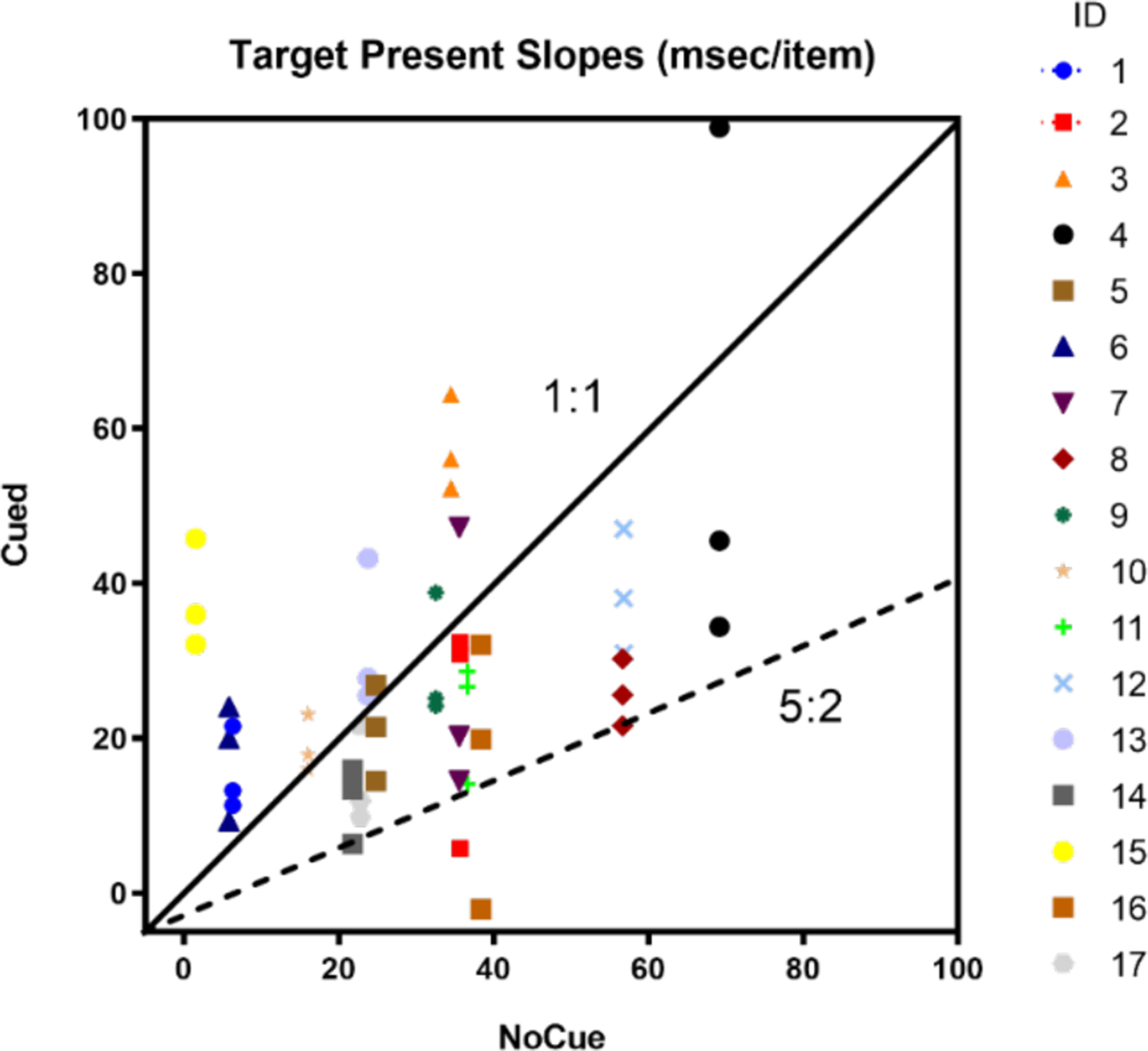
Target Present Slopes of Experiment 2: Cued vs. NoCue of multi-depth experiment (One data point represents one observer of each cue condition (Front, Back, Middle). The figure legend indicates tokens for different observers. The diagonal line represents the 1:1 ratio of cued vs. Nocue conditions while the dashed line represents the 5:2 ratio).
We can conclude that even if observers have the ability to direct attention to quite specific levels in depth, Experiment 2 failed to show a clear evidence that this ability could be used to guide search by observers in general. The color data raise a different possibility. It may be that the probabilistic cues used here are not effective. In a search for a 2 among 5, we know that there would be very effective guidance by color if half the items were red and we told the observers that the target would be red. The slope might not drop to one-half of the uncued condition, but it would drop (Egeth et al., 1984). Here, where the colors fall on a continuum, from red to yellow, observers may not be willing or able to use a cue that says that the target is merely most likely to be red, a bit less likely to be orange, and so forth. However, Utochkin, Khvostov & Wolfe, J. M. (2020) have shown that guidance is possible even if the display cannot be readily segmented into groups of items with and without the target color (for example). This suggests that the use of a continuum of colors or depths is not, by itself, the problem in Experiment 2. Accordingly, in Experiment 3, we simplified the design and were able to see that basic guidance by depth information is possible with these stimuli.
Experiment 3 –. Visual search in two depth planes
Since the effects of depth were equivocal in Experiment 2, we decided to check that depth guidance was possible with these stimuli in the simpler case of just two depth planes. The results showed that information about the target depth plane does allow observers to search more efficiently in a two-depth condition compared to a one-depth condition, replicating some earlier work. Previous work has not been completely clear on this point (Dent et al., 2012; Finlayson et al., 2013; Roberts et al., 2015). For the two-depth visual search task, Finlayson et al. found that, even when observers were informed of the depth of the target in advance, reaction time and search efficiency were not significantly different from presenting all stimuli at a single depth (Finlayson et al., 2013). However, Dent et al. found that depth information did guide visual search (Dent et al., 2012). Finlayson et al’s experimental design involved search for vertical T among Os and horizontally rotated Ts. Dent et al and Roberts et al’s tasks were to search for letters Z or N among other letters. The experimental stimuli used in the above two studies are similar, but the results are different (Roberts et al., 2015). Thus, some further data on this point seems useful.
Procedure
In Experiment 3, the experimental apparatus and tasks were essentially identical to Experiment 2 except that stimuli were confined to two depth planes. The task was the same search for a 2 among 5s with items presented at +15 and -15 arcmin disparity. To ensure that each observer had sufficient time to see the two depth planes, placeholders were presented to provide a 1500 msec preview for the observers before each trial. Before each trial, the observers were accurately informed that, if a target was present, it would be in the front plane or the rear plane for the two depth conditions. Target depth remained constant for a block of trials. A block consisted of 30 practice and 180 test trials distributed evenly over three set sizes (6, 12, and 24) with targets present on 50% of trials. 12 observers (mean age = 28.9 years, SD = 7.6, eight females) participated in this experiment. All gave informed consent and had normal visual acuity and stereopsis.
Results
Miss error rate averaged less than 10% in all three conditions. False positive rates were less than 2.5%. All error trials were excluded in the follow-up analysis. In addition, trials with RT greater than 3SD above the average were excluded as outliers (0.08%).
Figure 15 shows RTs as a function of set size for the three experimental conditions. It is clear that accurate information about depth improves search performance. This impression is supported by statistical analysis. A two-way repeated-measures ANOVA of target-present RTs revealed main effects of set size (F(2, 22) = 63.72, p < .001) and target depth (F(1.45, 16.00) = 10.39, p = .003), as well as an interaction effect between target depth and set size (F(2.36, 26.0) = 4.99, p = .011). These results showed significantly reduced RTs for two-depth conditions. The statistical analysis results of target-absent trials were similar. To further explore the interaction effect, paired t-tests on search slopes were conducted and the results showed that knowing the target was in the back plane produced search that was significantly more efficient than the single depth condition (t(11) = 3.56, p = .004). The difference between the target front and the single depth condition was marginally significant (t(11) = 2.16, p = .054). The difference between cue front and cue back conditions was not significant (t(11) = 1.01, p = .34). For the target-absent trials, the search slope of the target front condition was significantly lower than that of the single depth (t(11) = 2.64, p = .023), the difference between target back and the single depth conditions was marginally significant (t(11) = 1.99, p = .071), and the difference between target front and target back cues was not significant (t(11) = 0.59, p = .57).
Figure 15.

Results of Experiment 3: RT × set size functions of Two-depth vs. One-depth condition. Slopes of functions are given parenthetical next to condition names. Error bars indicate ±1 SEM.
Compared with presenting all stimuli on one depth plane, the reaction time and search efficiency were improved, both for target present and absent, after dividing the search display into two depths. If observers were able to restrict their search to only the relevant depth plane, then the depth-cued conditions should produce slopes that are half the single depth conditions. That is, for target present trials, observers only need to search through half of set size items, and for target absent trials, observers would be able to quit early since all items are evenly distributed on two depths. It can be seen from the average slopes in Figure 15 that this perfect guidance was not achieved. Figure 16 shows slopes for depth cued conditions plotted against uncued conditions for each observer. Some observers approximated perfect guidance with data lying on the 2:1 line. A smaller number seemed to produce no guidance, with data lying on the 1:1 line while the remainder fall in between. On average, observers can use simple depth information to guide though there may be interesting individual differences that could be investigated.
Figure 16.

Target Present Slopes of Experiment 3: Two-depth vs. One-depth (One data point represents one observer. The diagonal line represents the 1:1 slopes ratio of OneDepth vs. TwoDepth conditions, while the dashed line represents the 2:1 ratio).
Discussion & Conclusion
This paper adds to our understanding of the interaction between attention and the perception of depth from stereoscopic disparity. The most novel contribution of this work is found in Experiment 1. Those results show that, at least, some human observers can use disparity information to direct attention to a quite narrow slab of 3D space. The experiment shows that the Sun et al (2016a,b) centroid method works in stereoscopic depth as it does in the color domain. The results did not need to come out as they did. When the centroid method was tried in orientation, performance was not good (Inverso et al., 2016). It might have been possible to direct attention only more coarsely on the basis of depth even if fine grain discrimination was possible for attended stimuli. This is the case for other basic features. Continuing with orientation as an example, attentional mechanisms seem limited to orientations on the order of 15 deg in visual search while orientation acuity is less than 1 deg (depending on the stimuli) (Foster & Ward, 1991). Something like this may be true for depth as a feature as well. It is extremely unlikely that the ability to select a depth plane could be as fine as hyperacute stereoacuity (Westheimer, 2013). Nevertheless, the results of Experiment 1 show that, for the centroid task, attention in depth is not limited, for example, to near and far depth.
Experiment 2 attempted to get observers to deploy this relatively fine-grained set of attentional filters in the service of the guidance of visual search. We asked our observers to use something like an attentional gradient and to either start from the back of the space and work forward or vice versa. The results provide some evidence for such guidance but that evidence is weak. There are a number of possible explanations of this result. First, the experiment may be underpowered because the guidance effect, if it is real, proves to be weaker than expected. If the depth cues could have been used optimally, like ‘pure’ filter for depth in Experiment 1, then the slope in the cued conditions should have been markedly shallower than the slopes in the uncued condition. This was not found. The hypothesis that Os are not able to direct their attention depth by depth, in general, is disproven by Experiment 3. In Experiment 2, effective guidance was also not found for the color control condition, even though there is no serious doubt that color signals can guide attention. This raises the possibility that probabilistic cues, like the ones we used, are not effective. Alternatively, it is always possible that observers simply did not choose to make the effort to use the cue. Unlike a simple cue (look for red 2s), using these more complex cues seems to require some effort. The potential benefit of that effort is some hundreds of msec per trial. This fraction of a second may be very salient to those who study such things, but it may not be worth the effort for the observers. We are not suggesting that observers made a deliberate calculation of the RT-effort tradeoff. It would be more likely that a naïve observer simply did not notice the benefit. It is also possible to argue that guidance by depth plane is unnatural, in the sense that there are not many situations where you would limit search on the basis of depth. Searching for berries within convenient reaching distance could be an example. More typically, observers might devote their attention to a visible surface, which might or might not lie in the frontal plane in depth (He & Nakayama, 1992).
As noted, our final experiment was a test of the hypothesis that no guidance by depth was possible with these stimuli. As discussed earlier, depth guidance has been the subject of some debate in the literature [e.g. (Finlayson et al., 2013)]. Experiment 3 serves to show that depth guidance is possible with the stimuli used in Experiment 2. If we limit the cues to near and far, we can see clear evidence of guidance.
The overall conclusion from these studies is that attention can be directed to planes in depth but that this ability does not translate easily to guidance of visual search. In visual search, guidance by depth appears to be like other forms of guidance, relatively coarse and categorical (Wolfe et al., 1992). The strength of these conclusions is tempered by some limitations in the study. The experiments may be underpowered in light of the apparent size of the guidance effects. Moreover, it is possible that changes in the method might improve guidance. Observers could be rewarded more vigorously for using the depth cues and that use might improve with more extensive practice. Still, the results appear consistent with the way that depth cues are used in the world. It would be common to cue a colleague to look for something nearby or farther away. It would be less likely to cue to a more specific depth plane, even if that capability does appear to exist.
Supplementary Material
Figure 2.

Exemplar stimuli used in centroid estimation experiment (cross fusion), the red round dot is the centroid of three square dots that lie at the target depth
Acknowledgement
This research was supported in part by NIH (EY017001) to JMW, National Natural Science Foundation of China (U20B2062, U19B2032) to BZ, and National Natural Science Foundation of China (61960206007) to YL.
APPENDIX: Estimation of Attention Filter Weights
The accuracy of centroid estimation is affected by random errors and inherent error biased to the default position (x0, y0) (the centroid estimated by observers is biased to a fixed position). To obtain the accurate attention filter under different experimental conditions, the above errors need to be modeled. When only the random response error is considered, the estimation of the centroid coordinates in trial j can be expressed by the following formula:
| (1) |
| (2) |
Where is the x coordinate of the estimated centroid in trial j, is the depth of dot i in trial j, is the filter weight of the corresponding depth, xi(j) is the x coordinate of dot i in trial j, where the random response error Nx(j) and Ny(j) are two independent random variables with normal distribution (mean = 0, SD = σ2). Equations (1) and (2) are the formulas for the centroid estimation of 24 dots after considering random errors.
Inherent error represents the assumption that during centroid estimation, observers do not completely rely on the current experimental stimulus, but tend to a default position. The influence of the current stimulus on centroid estimation is called Data-drivenness (D) (Sun et al., 2016b), and the influence of the default position can be expressed as (1-D). If D=1 indicates that the observer completely depends on the experimental stimulus to judge the centroid, and the other extreme D=0 indicates that the observer’s centroid estimation is the default position without considering stimuli at all.
Then, the estimated centroid can be expressed as:
| (3) |
| (4) |
The above two equations can be further rewritten as:
| (5) |
| (6) |
Where, (x0, y0) is the fixed default position that observers’ response is biased to, for t = 1,2, … ,8 (there are 8 depth planes and 3 dots in each depth), Xt(j) represents the sum of x coordinates of three dots on depth t in trial j. Yt(j) is the sum of y coordinates of three dots on the depth t. For t = 9 or 10, X9(j) = 1, X10(j) = 0, Y9(j) = 0, Y10(j) = 1.
| (7) |
Where A is the sum of the weights of all dots.
| (8) |
Equations (5) and (6) are linear equations and share the weight Wt, t = 1,2, … ,8. The above is the estimation of one trial. Considering that the whole experiment has Ntrail trials, a Ntrail × 10 matrix X was used to save x coordinates in all trials, where the elements in row j column t are Xt(j). Similarly, all Yt(j) is saved with matrix Y. Matrix X and Y have the same dimension. L represents the superposition matrix of the two matrices, where j = 1,2, … ,2Ntrail, t = 1,2, … ,10,
| (9) |
Similarly, by concatenating and , for j = 1,2, … ,2Ntrail,
| (10) |
Thus, equations (5) and (6) can be rewritten as:
| (11) |
Where N represents random error with zero mean and σ2 standard deviation.
Then, the estimation of the weight can be obtained by minimizing the following equation:
| (12) |
The above formula is a non-negative restricted least square problem, which can be solved with Matlab function lsqnonneg (Lawson & Hanson, 1995).
To estimate , we take
| (13) |
To ensure that sums to 1. Finally, the following statistics are used to estimate (x0, y0)
| (14) |
| (15) |
| (16) |
Footnotes
This work was done while the first author was in Visual Attention Lab, Harvard Medical School and Brigham & Women’s Hospital, United States.
Contributor Information
Bochao Zou, School of Computer and Communication Engineering, University of Science and Technology Beijing, China1.
Yue Liu, Beijing Engineering Research Center of Mixed Reality and Advanced Display and School of Optoelectronics, Beijing Institute of Technology, China.
Jeremy M. Wolfe, Visual Attention Lab, Harvard Medical School and Brigham & Women’s Hospital, United States
References
- Brainard H, D. (1997). The Psycholysics Toolbox. Spatial Vision, 10(4), 433–436. 10.1007/s13398-014-0173-7.2 [DOI] [PubMed] [Google Scholar]
- Breitmeyer B, Ogmen H, & Öğmen H (2006). Visual masking: Time slices through conscious and unconscious vision Oxford University Press. [Google Scholar]
- Busettini C, Fitzgibbon EJ, & Miles FA (2001). Short-latency disparity vergence in humans. Journal of Neurophysiology, 85(3), 1129–1152. [DOI] [PubMed] [Google Scholar]
- Caziot B, & Backus BT (2015). Stereoscopic Offset Makes Objects Easier to Recognize. PloS One, 10(6), e0129101. 10.1371/journal.pone.0129101 [DOI] [PMC free article] [PubMed] [Google Scholar]
- Caziot B, Valsecchi M, Gegenfurtner KR, & Backus BT (2015). Fast perception of binocular disparity. Journal of Experimental Psychology: Human Perception and Performance, 41(4), 909. [DOI] [PubMed] [Google Scholar]
- de la Rosa S, Moraglia G, & Schneider B. a. (2008). The magnitude of binocular disparity modulates search time for targets defined by a conjunction of depth and colour. Canadian Journal of Experimental Psychology = Revue Canadienne de Psychologie Expérimentale, 62(3), 150–155. 10.1037/1196-1961.62.3.150 [DOI] [PubMed] [Google Scholar]
- Dent K, Braithwaite JJ, He X, & Humphreys GW (2012). Integrating space and time in visual search: How the preview benefit is modulated by stereoscopic depth. Vision Research, 65, 45–61. 10.1016/j.visres.2012.06.002 [DOI] [PubMed] [Google Scholar]
- Duan Y, Thatte J, Yaklovleva A, & Norcia AM (2021). Disparity in Context : Understanding how monocular image content interacts with disparity processing in human visual cortex. NeuroImage, 237(February 2020), 118139. 10.1016/j.neuroimage.2021.118139 [DOI] [PMC free article] [PubMed] [Google Scholar]
- Egeth HE, Virzi R. a, & Garbart H (1984). Searching for conjunctively defined targets. Journal of Experimental Psychology. Human Perception and Performance, 10(1), 32–39. 10.1037/0096-1523.10.1.32 [DOI] [PubMed] [Google Scholar]
- Finlayson NJ, Remington RW, Retell JD, & Grove PM (2013). Segmentation by depth does not always facilitate visual search. Journal of Vision, 13(2013), 1–14. 10.1167/13.8.11.doi [DOI] [PubMed] [Google Scholar]
- Foster DH, & Ward PA (1991). Asymmetries in oriented-line detection indicate two orthogonal filters in early vision. Proceedings of the Royal Society of London. Series B: Biological Sciences, 243(1306), 75–81. [DOI] [PubMed] [Google Scholar]
- Godwin HJ, Menneer T, Liversedge SP, Cave KR, Holliman NS, & Donnelly N (2017). Adding depth to overlapping displays can improve visual search performance. Journal of Experimental Psychology: Human Perception and Performance, 43(8), 1532. [DOI] [PubMed] [Google Scholar]
- Godwin HJ, Menneer T, Liversedge SP, Cave KR, Holliman NS, & Donnelly N (2020). Experience with searching in displays containing depth improves search performance by training participants to search more exhaustively. Acta Psychologica, 210(April), 103173. 10.1016/j.actpsy.2020.103173 [DOI] [PubMed] [Google Scholar]
- Greenhouse SW, & Geisser S (1959). On methods in the analysis of profile data. Psychometrika, 24(2), 95–112. [Google Scholar]
- Horowitz TS (2005). Visual search: The role of memory for rejected distractors. In Neurobiology of attention (pp. 264–268). Elsevier. [Google Scholar]
- Horowitz TS, & Wolfe JM (1998). Visual search has no memory. Nature, 394(6693), 575–577. [DOI] [PubMed] [Google Scholar]
- Inverso M, Sun P, Chubb C, Wright CE, & Sperling G (2016). Evidence against global attention filters selective for absolute bar-orientation in human vision. Attention, Perception, & Psychophysics, 78, 293–308. 10.3758/s13414-015-1005-3 [DOI] [PubMed] [Google Scholar]
- Lawson CL, & Hanson RJ (1995). Solving least squares problems SIAM. [Google Scholar]
- Levitt H (1971). Transformed Up‐Down Methods in Psychoacoustics. The Journal of the Acoustical Society of America, 49(2B), 467–477. 10.1121/1.1912375 [DOI] [PubMed] [Google Scholar]
- Marrara MT, & Moore CM (2000). Role of perceptual organization while attending in depth. Percept Psychophys, 62(4), 786–99. 10.3758/BF03206923 [DOI] [PubMed] [Google Scholar]
- McSorley E, & Findlay JM (2001). Visual search in depth. Vision Research, 41(25–26), 3487–3496. 10.1016/S0042-6989(01)00197-3 [DOI] [PubMed] [Google Scholar]
- Nakayama K, & Silverman GH (1986). Serial and parallel processing of visual feature conjunctions. Nature, 320(6059), 264–265. 10.1038/320264a0 [DOI] [PubMed] [Google Scholar]
- O’Toole AJ, & Walker CL (1997). On the preattentive accessibility of stereoscopic disparity: Evidence from visual search. Perception & Psychophysics, 59(2), 202–218. [DOI] [PubMed] [Google Scholar]
- Ogawa A, & Macaluso E (2015). Orienting of visuo-spatial attention in complex 3D space: Search and detection. Human Brain Mapping, 36(6), 2231–2247. 10.1002/hbm.22767 [DOI] [PMC free article] [PubMed] [Google Scholar]
- Plewan T, & Rinkenauer G (2018). Surprising depth cue captures attention in visual search. Psychonomic Bulletin and Review, 25(4), 1358–1364. 10.3758/s13423-017-1382-9 [DOI] [PubMed] [Google Scholar]
- Plewan T, & Rinkenauer G (2020). Allocation of attention in 3D space is adaptively modulated by relative position of target and distractor stimuli. Attention, Perception, and Psychophysics, 82(3), 1063–1073. 10.3758/s13414-019-01878-2 [DOI] [PubMed] [Google Scholar]
- Plewan T, & Rinkenauer G (2021). Visual search in virtual 3D space: the relation of multiple targets and distractors. Psychological Research, 85(6), 2151–2162. 10.1007/s00426-020-01392-3 [DOI] [PMC free article] [PubMed] [Google Scholar]
- Reeves A, & Lynch D (2017). Transparency in stereopsis: parallel encoding of overlapping depth planes. Journal of the Optical Society of America A, 34(8), 1424. 10.1364/josaa.34.001424 [DOI] [PubMed] [Google Scholar]
- Reis G, Liu Y, Havig P, & Heft E (2011). The effects of target location and target distinction on visual search in a depth display. Journal of Intelligent Manufacturing, 22(1), 29–41. 10.1007/s10845-009-0280-z [DOI] [Google Scholar]
- Richards W (1970). Stereopsis and stereoblindness. Experimental Brain Research, 10(4), 380–388. [DOI] [PubMed] [Google Scholar]
- Richards W (1971). Anomalous stereoscopic depth perception. JOSA, 61(3), 410–414. [DOI] [PubMed] [Google Scholar]
- Roberts KL, Allen HA, Dent K, & Humphreys GW (2015). Visual search in depth: The neural correlates of segmenting a display into relevant and irrelevant three-dimensional regions. NeuroImage, 122, 298–305. 10.1016/j.neuroimage.2015.07.052 [DOI] [PMC free article] [PubMed] [Google Scholar]
- Sarno DM, Lewis JE, & Neider MB (2019). Depth benefits now loading: Visual working memory capacity and benefits in 3-D. Attention, Perception, and Psychophysics, 81(3), 684–693. 10.3758/s13414-018-01658-4 [DOI] [PubMed] [Google Scholar]
- Sun P, Chubb C, Wright CE, & Sperling G (2016a). Human attention filters for single colors. Proceedings of the National Academy of Sciences of the United States of America, 113(43), E6712–E6720. 10.1073/pnas.1614062113 [DOI] [PMC free article] [PubMed] [Google Scholar]
- Sun P, Chubb C, Wright CE, & Sperling G (2016b). The centroid paradigm: Quantifying feature-based attention in terms of attention filters. Attention, Perception & Psychophysics, 78(2), 474–515. 10.3758/s13414-015-0978-2 [DOI] [PubMed] [Google Scholar]
- Theeuwes J, Atchley P, & Kramer AF (1998). Attentional control within 3-D space. Journal of Experimental Psychology: Human Perception and Performance, 24(5), 1476–1485. 10.1037/0096-1523.24.5.1476 [DOI] [PubMed] [Google Scholar]
- Utochkin IS, Khvostov VA, & Wolfe JM (2020). Categorical grouping is not required for guided conjunction search. Journal of Vision, 20(8), 30. [DOI] [PMC free article] [PubMed] [Google Scholar]
- Westheimer G (2013). Clinical evaluation of stereopsis. Vision Research, 90, 38–42. [DOI] [PubMed] [Google Scholar]
- Wheatstone C (1838). Contributions to the Physiology of Vision. Part the First. On Some Remarkable, and Hitherto Unobserved, Phenomena of Binocular Vision. Philosophical Transactions of the Royal Society of London, 128(1838), 371–394. 10.1098/rstl.1838.0019 [DOI] [Google Scholar]
- White KD, & Odom JV (1985). Temporal integration in global stereopsis. Perception & Psychophysics, 37(2), 139–144. [DOI] [PubMed] [Google Scholar]
- Wolfe JM (2010). Visual search. Current Biology, 20(8), 346–349. 10.1016/j.cub.2010.02.016 [DOI] [PMC free article] [PubMed] [Google Scholar]
- Wolfe JM, Friedman-Hill SR, Stewart MI, & O’Connell KM (1992). The role of categorization in visual search for orientation. Journal of Experimental Psychology: Human Perception and Performance, 18(1), 34. [DOI] [PubMed] [Google Scholar]
- Wolfe JM, & Horowitz TS (2017). Five factors that guide attention in visual search. Nature Human Behaviour, 1(3), 0058. 10.1038/s41562-017-0058 [DOI] [PMC free article] [PubMed] [Google Scholar]
Associated Data
This section collects any data citations, data availability statements, or supplementary materials included in this article.