

Abstract
The present work presents an algorithmic approach to determine the optimal starting point for any complex geometry draping processes. The time-efficient Kinematic Draping Simulation (KDS) is used to assess the drapability of a geometry depending on many different starting points. The optimization problem is then solved by applying Particle Swarm Optimization (PSO). The proposed methodology is applied to and validated with complex geometry and a common part of the automobile industry: the B-Pillar geometry. The results show that the PSO algorithm may improve random search up to 78 times. After several experiments, PSO particles have discrete coordinates and are located at optimum global and local regions most of the time, leading to solutions for complex objective functions. The global solution is such that the starting point is located near the geometrical centre of the B-Pillar. The novelty of the work is evident: it uses optimization for a real engineering application, and it draws pattern-related conclusions for other geometries. Experimental results are shown to be consistent with simulation results.
Keywords: Particle swarm optimization, Kinematic draping simulation, Starting point, B-Pillar
Particle swarm optimization; Kinematic draping simulation; Starting point; B-Pillar
1. Introduction
Global mobility is increasing due to growing globalization and higher demands in different societies. At the same time, the restrictions to reduce greenhouse gases, like CO2, are increasing. The mobility sector is already the second biggest contributor to CO2 emissions [1]. One way to reduce emissions is by reducing the weight of vehicles, like automobiles, ships or planes. Reducing the weight of vehicles can be achieved through the use of lightweight materials. FRC are among the most desirable lightweight materials due to their high mechanical properties and low density compared to other lightweight materials like aluminium. Despite these advantages, the widespread use of FRC is small due to a complex production process which causes high costs of FRC parts. One of the most important production steps within the process chain of FRC is the molding of the composite part, which can account for up to 50% of the parts costs [2, 3, 4]. During preforming, the draping of textiles is a crucial step [5]. A cost-intense trial-and-error approach often dominates the design of the draping process. One way to reduce those costs is the use of draping simulations. The simulations enable the developer to reduce material and labor costs during a shortened and development process. Subsequently, fewer molding tools and textile reinforcement materials need to be processed to find the ideal set-up. A Draping Simulation is defined in the literature as the simulation of the forming process the textile undergoes to mold from a planar geometry into the desired 3D shape [6]. It is generally kinematic or mechanical, depending on the approach being based in constitutive models for higher precision accurate values or only geometrical characteristics for an approximated prediction. Compared to FE-draping simulations, Kinematic Draping Simulations (KDS) need lower computational resources at the cost of accuracy. Nevertheless, for a short assessment of the drapability of a certain geometry, the KDS is a proper tool. One challenge in draping, which occurs in the KDS, is finding a suitable starting point. The results of KDS are strongly dependent on the starting point of the simulation, which is equivalent to the actual draping dependence to the starting point [7]; Changing the starting point of the draping influences the outcome such as fibre orientation or the occurrence of defects like folds. The use of an optimization method can approach the challenge of finding a suitable starting point. Because varying the starting point conducts to further variation of the distribution of the shear angles, this starting point must be optimized to minimize the distribution of the shear angle. More precisely, the aim is to minimize shear deformation over the whole geometry and avoid critical deformation areas, using the fastest and most efficient process possible. This problem was addressed by Skordos et al. [8] but was not entirely solved since no conclusions are taken about the expected optimal starting point for other geometries. Also, in their work [8], the authors applied a Genetic Algorithm (GA) in a draping simulation. Thus, the present work is aimed to optimize the starting point of a KDS using PSO. PSO [9] is one of the most promising optimization methods due to its simplicity, efficiency, and problem independence [10]. It is implemented in different forms to optimize processes and design. PSO is modified and even hybridized with other methods to not be more stuck in the local optima. PSO might also improve costs through higher efficiency since PSO has been proven to evaluate less than GA [11]. The use of PSO to fill the existing gap in KDS has to be explored to determine its utility to predict the best starting point according to a specific criterion, reducing time and energy costs. Therefore, the proposed work is designed to investigate PSO in a KDS of a B-Pillar geometry. This geometry derives from a real B-Pillar and is chosen due to its complex geometry and possible application as an FRC part. According to Kaufmann [12], the starting point of the optimized draping process of any geometry is expected to be located at a certain region of such a geometry where its curvature is equal to zero. This is a hypothesis that is tested in this work. The present work is organized by the following sequence: The next section is a review of the related literature; a state-of-the-art exposition in regards to PSO comes next; the methodology section presents the theoretical framework explaining how PSO is implemented in the KDS and an exposition on the objective criteria and the conditions of the experiments to validate the results obtained from the simulation; the results regarding both simulations and experiments are then exposed and discussed; the main conclusions from the study are drawn at the end of the work. The following questions are expected to be answered:
-
1.
Where is the starting point of the optimized KDS process located relatively to the B-Pillar geometry and according to the selected criterion?
-
2.
Which are the population size and PSO variation kinds of optimizers in which KDS optimization of a B-Pillar geometry leads more quickly to the optimum global solution?
-
3.
How does the simulation compare to experimental results?
2. Review of the literature
Draping simulations can have different based models. Robertson et al. [13] used a model based on a fisherman's net with fixed length and nodes. It is explained that there are three tests of significance: the uniqueness of the nodal location, the angles between fibres, and how much significant the grid size and number of nodes are for the location of the nodes. Also, another model commonly used is the mass-spring model, used for the first time by Provot [14]. The mass-spring model is different from the fisherman's net based model. In the first model, the internal energy due to the motion of the several masses and springs are potential energy. As the models in numerical simulations are not ideally realistic, some assumptions are taken as, for example, neglecting the bending stiffness, material non-linearities, frictional effects or process conditions [15]. Studies were done with different geometries, such as: Double Dome [16], hemisphere [17, 18, 19], tetrahedron [17, 18], square box [20], pyramids and round boxes [21, 22]. With the constant advance of technology and generally shorter product life cycles, industrial processes require more adjustments in part quality, geometry, cycle time and cost. So, “trial and error” proceedings would be too time-consuming and costly, causing impracticalities [23]. The importance of using optimization methods has been seen as mandatory to reduce this problem by accelerating design and process planning. In this regard, several optimization tasks have been performed. Notwithstanding, due to the expansion of both optimization and draping simulation fields, the literature is vast of applications. The solution often is to recur to surrogate-based optimization models [24] and single or multiobjective-optimization [25] non-traditional methods to optimize different parameters in both kinematic and mechanical draping simulations. In work developed by Mozafary and Payvandy [26], the aim was to characterize parameters of a mass-spring model using PSO and FAST test, where the variables are mainly the natural length of spring, the super elasticity rate and the mesh topology. For these applications, the Taguchi method is used to assist their comprehension [27]. Mozafary and Payvandy [28] used Imperialist Competitive Algorithm (ICA) to optimize stiffness coefficient, damping coefficient, elongation rate, topology mesh and natural spring length, with the assistance of various experiences optimized with the Taguchi method and using an objective function. Mongus et al. [29] used as a hybrid optimization method, in which the evaluation function was defined not only by the comparison between the actual textile and the simulation textile but also by the contour characterization, which is irregular. This causes the problem to become multi-objective. Another work was done and presented by Zimmerling et al. [30], which aims to minimize the shear angle distribution induced by the geometry during draping operation, using other Artificial Intelligence methods. The methodology used is based on Reinforcement Learning (RL), where some tests verified through images are initially trained by a Convolutional Neural Network (CNN) to create the forming results. A second CNN evaluates the impact and computes some pressure pads' positions in the manufacturing process. High computation costs using RL in the initial phase could be compensated in the long term.
3. Particle swarm optimization
PSO [9, 31] is a technique that was inspired by social behaviours like bird flocking, fish schooling and particularly in swarming theory. PSO is mainly based on updating multidimensional velocities and positions of each population particle i, at each generation t, as it is shown in (1) and (2).
| (1) |
| (2) |
where is the velocity of a particle, is the inertia weight, which was introduced in later publications [32], and are cognitive and social coefficients, respectively, is the best position of each particle position among all particles and generations between first among all the generations between the first and , is the best position among all particles and generation between the first generation and generation t, and and are normalized values at random. PSO has received more attention since its first implementation in 1995, leading the scientific community to verify some systematic issues resulting in the most known premature convergence and consequently developing variations of PSO. In 1999, Maurice Clerc introduced a constriction factor [33] related to , . In the following years, two terms appeared in the literature – and – respectively, the best position of a certain particle across all the generations and the best position of all the particles across all the generations. These terms are used later within this paper. It was shown that the discrete-time PSO presents could be generalized to a continuous-time [34] from an analytical point of view. K is determined by controlling the exploration and exploitation, and it is multiplied by the righthand side of (1), turning the resulting equation a variation of the original one. RPSO [35] is a PSO variation that chooses a particle and updates its position at random in the search space with a step time equivalent to the number of particles in the swarm, once at a time. In 2006, Van der Bergh [35] demonstrated that PSO is a local but not a global search algorithm. However, RPSO has been proven to be a global search method because it samples the particles at random in each generation. Apart from the variation, these PSO single objective variant methods generally have a generalized flowchart, which is represented in Figure 1. The following steps regard the sequence from the start to the end of the same flowchart [36, 37]:
-
1.
Initialization: In general, the variables that need an initial setup are the maximum number of generations, inertia, individual and social cognitive weights, the swarm size, the number of dimensions, constrain factor, initial generation, initial positions and velocities (which are stated in the literature to be equal) and boundary values for the variables, commonly included inertia.
-
2.
Fitness evaluation: According to the position of each particle position , is calculated through , where is the evaluation function.
-
3.
Update and : Once a particle is evaluated according to , is then updated with in which . When the entire current swarm is evaluated, is updated using in which and .
-
4.
Update velocity and position: Velocity and position are updated according to the method used, but for classic PSO, the equations are described by (1) followed by (2).
-
5.
Evaluate if it has reached to the last generation: If the algorithm has reached the last generation, a variable previously set up by the user, PSO stops. Otherwise, it continues the loop, returning to step 2.
Figure 1.
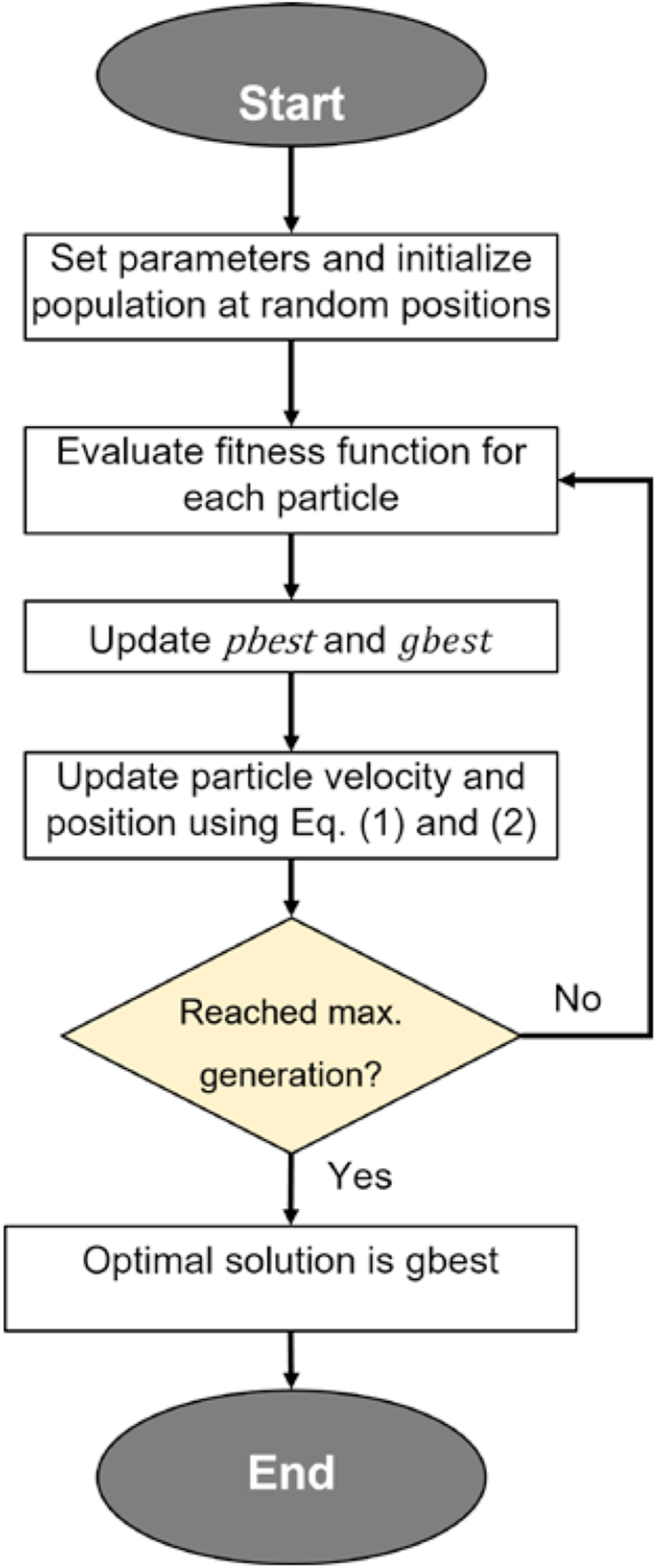
Flowchart for the classic PSO algorithm.
PSO is a widely used method in several applications along with Genetic Algorithm (GA). They were reported [10, 38] as similar techniques because they are population based and optimal solutions are updated through the generations; notwithstanding, PSO was demonstrated [10, 39] to be a more straightforward method to implement, and the information is also shared through the particles of the same generation.
A study [11] was also statistically demonstrated that PSO needs fewer evaluation functions in relation to GA. Other advantages are reported to be the non-assumption of continuity and differentiability of the objective function, that computing the gradient of the error function is not needed, optima starting points are not necessary, and the problem independent character [10]. Nowadays, the development of optimization algorithms is still a topic of great interest. For example, Zeng et al. [39] have recently introduced a new competitive strategy for whale optimization algorithm in order to improve convergence. Also, Liu et al. [40] have used a Gaussian white noise with adjustable intensity for the randomization of the PSO particles acceleration, improving the global convergence of the algorithm. Still, all optimization techniques are bounded by the No Free Lunch Theorem [41], and PSO is not an exception. Such a Theorem states that no algorithm performs better than another when considering all classes of problems. Therefore, investigations should be done to understand better PSO and its performance over other candidate algorithms among engineering optimization problems. PSO has been studied by the scientific community and is considered one of the leading population-based intelligent algorithms. Even in the most recent years, and as shown in Figure 2, it is possible to verify the interest in applying PSO over several areas. Still, in the literature review [42], it is possible to verify some future work statements as parameter sensitivity, convergence to local optima or subpar performance in multi-objective optimization for higher dimensional problems. In this research, this technique is used as a basis. Further information about the variation from this technique and its applied changes are presented in the methodology section.
Figure 2.

Number of publications per year related to PSO. Source: Google Scholar.
4. Methodology
As exposed previously, one of the current problems in KDS is defining the starting point and the orientation of the mesh to facilitate the operator in draping tasks. In this work, PSO is used only to define the starting point whose position on a B-Pillar geometry is to be placed so that the objective function concerning a selected criterion is minimized. The orientation of the textiles cannot be changed when the draping process is designed since the textile layup was defined previously. This is why an orientation change is not considered in optimization. The KDS algorithm presented by Kaufmann [12] is used in this work. According to it, the starting point is the most influencing parameter that directly affects the position of the rest of the particles. A geometry of size is assumed as an increment and . The shear angle value can be generally defined as in (3).
| (3) |
are discretized points of the geometry. In this work, in order to avoid unnecessary computational time and to simplify the used mathematical notation, the increments m and n are assumed as integers. A representation of the shear angle is illustrated in Figure 3. In this Figure, the relation helds. In fact, the length of the vectors is equal and constant for any point of the mesh. This constant is equal to , that will be used in the next equations and its physical meaning can be visualized in Figure 4. The value can be seen as the length between the middle of two crossing points within a plain weave. The higher the value is, the faster is the simulation. From the starting point and the nearest points along with a defined orientation, further points are computed according to (4), in which being the surface of the given geometry, is the third coordinate. The surface of the geometry is achieved from the 3D model represented in Figure 3.
Figure 3.

Illustration of the B-Pillar (left) and shear angle in the context of KDS (right).
Figure 4.

Physical meaning of the -value in the KDS, for an exemplary plain weave.
The pre-processing is done in the following way: several points of the external surface of the given geometry are extracted; the points in the base of the model are removed; a smooth interpolation is carried out.
| (4) |
Let a particle from PSO be defined as Then, is the starting point for which is tested, being these coordinates discretized values. The output of an objective function , given the design variables and , can be written as . From the definition of shear angle, formulating can be done according to different criteria. In this work, the considered criteria are:
-
•
Criteria type A1 – minimizing the maximum shear angle in Ω
-
•
Criteria type A2 – minimizing the sum of all shear angles in
-
•
Criteria type A3 – minimizing the sum of the square of all shear angles in
-
•
Criteria type A4 – minimizing the sum of all shear angles in where
-
•
Criteria type A5 – minimizing the sum of the square of all shear angles in
-
•
Criteria type A6 – minimizing the count of shear angles whose absolute value is above a threshold value in
Criteria A1 and A2 are specific cases of A4 when and , respectively, and criterion A3 is a specific case of A5 when The difference between A4 and A5 is that in A5 the values for shear angles are squared. The definition of is dependent of if it is considered the displacement of the relevant geometry region or if it is also considered the flat region. If considered the second case, , where represents the available domain where PSO particles are sampled. However, in this work, shear angles on points in the flat region are not considered. The map of each domain is visually represented in Figure 5. From the types A1–A6, criteria C1–C6 are formulated, being these listed in Table 1 and the objective functions used for the analysis of the results.
Figure 5.

Visual identification of the PSO domain and shear angle evaluation domain.
Table 1.
List of used criteria as objective functions of the minimization problem.
| Criteria label | Based criteria type |
|---|---|
| C1 | A3 or A5 with |
| C2 | A6 with |
| C3 | A1 or A4 with |
| C4 | A2 or A4 with |
| C5 | A4 with |
| C6 | A4 with |
Having the objective function been formulated, the flow chart in Figure 1 can be adapted, originating the flowchart presented in Figure 6.
Figure 6.

Flowchart for the overall problem.
Due to the limitations of the solver, the chosen decision criterion and the time needed to spend in practice, a value for the parameter K of 6 is chosen as a compromise between calculation time and accuracy.
As it was presented in Section 2, there are several methods in which original PSO is presented as a working principle. For this work, a set of variations of the original PSO were selected and listed in Table 2. In this table, the known name of the algorithm and its reference in the literature is given in the first column, the reference of the algorithm is an abbreviation presented in the second column, the changes to the flowchart in Figure 6 and the used hyperparameters used to perform the algorithm are given by the information in the last two columns.
Table 2.
List of used PSO variants.
| PSO algorithm | Abbreviation | Changes to flowchart in Figure 1 | Hyperparameter values for test performance | Hyperparameter dependence |
|---|---|---|---|---|
| RPSO [35] | M1 | A particle (where t is the current generation and P is the population size) is randomly sampled in the domain before Step 5 | Particles per generation to sample: 1 | Low |
| PSO with constriction factor [34] | M2 | – | – | Very low |
| PSO + Genetic Algorithm [43] | M3 | Genetic Algorithm is performed before Step 5 | High | |
| GA performance per generation: 1 | ||||
| PSO + Cuckoo Search (CS) [44] |
M4 | Position (in Step 4) is calculated based on the following equation: | CS performance per generation: 1 | Low |
| where is calculated using (2), is a random number and is calculated using Cuckoo-Search related equations (in [44]) | ||||
| PSO + Firefly Algorithm (e.g. [45]) | M5 | The population is split into two subpopulations SP1 and PS2. Firefly Algorithm is performed on PS1 and PSO equations (Step 4) on SP2 |
|
Very high |
M2 represents the algorithm provided by the original flowchart of Figure 1. For all the algorithms except M5, the population size is 12, and .
Having all the PSO parameters, PSO algorithm, value and objective function been selected, the overall algorithm is ready to be performed. The simulation results are given in the next section, and the comparison between all the variables is now referenced.
5. Results and discussion
5.1. Optimization results of the starting point for different criteria
From the configurations listed in the previous section, C1–C6 criteria are tested using M2 with a swarm population of 24 particles. A total of 10 generations of particles are reproduced during 30 experiments. A two-axis colourmap is considered for visualization, whose spectra vary from colder to hotter colours and transparency variations are used. Regions whose starting points minimize shear angle through some criteria are marked with a colder colour, whereas those which lead to higher shear angle values are marked with a hotter colour. In its turn, local and global solutions correspond to less transparent regions. These may be observed according to the frequency of the particles in a specific region; therefore, if a region is high frequently populated, a local solution is most likely to be there. Figure 7 shows such a mapping, considering each criterion in Table 1. The scores in Figure 7 are then computed using the expressions for in the methodology section.
Figure 7.

2D colormap for criteria C1 to C6.
With C1, it is possible to observe a global solution nearly at the centre of the B-Pillar geometry. In contrast, much less probable solutions are located in the neighbours of such a geometry. Considering other criteria (C2–C6), the same observation is possible to be taken. Table 3 lists the optimized values for each criterion and the starting point locations as well.
Table 3.
List of global optima considering different criteria.
| Criterion | Minimized value | X | Y |
|---|---|---|---|
| C1 | 117.5 | 92 | 111 |
| C2 | 222 | 96 | 102 |
| C3 | 30.49 | 92 | 111 |
| C4 | 5.704 | 93 | 107 |
| C5 | 13.90 | 93 | 107 |
| C6 | 28.78 | 92 | 105 |
It is possible to confirm that the minimized solution is obtained for a starting point that is located almost in the same region, almost independently of the used criterion. Moreover, Figure 8 shows the obtained shear-angle mapping when considering the starting point with coordinates (92,111), representing the optimized one for criterion C1. This point is labelled in this work as SPO.
Figure 8.

Draping simulation with an optimum starting point.
5.2. Study of different algorithms for criterion C1
Testing different optimization configurations lead to the results of this subsection. Different PSO hybridizations are considered, listed previously in Table 2. Efficiency values for the search of the optimized point near the centre region of the geometry are listed in Table 4 for each PSO variation, in the form of probability percentage.
Table 4.
PSO variant comparison by efficiency ratio.
| PSO variant from Table 2 | Probability of being at SPO | Efficiency ratio |
|---|---|---|
| M1 | 4.56% | 67 |
| M2 | 2.67% | 39 |
| M3 | 0.93% | 14 |
| M4 | 2.45% | 36 |
| M5 | 5.38% | 78 |
This percentage represents how many instances of particles are near the optimum solution compared to the possible domain. For comparison, the expected value of this probability for a pseudo-random methodology is equal to 0.068%. The efficiency ratio is then given by dividing the respective tabled value by the reference value. Each method is run through 10 experiments.
The results show that the methods improve efficiency to be 14–78 times faster depending on the used PSO variation, when compared to random search for the optimal starting point. This means that, according to the experiments, global best is expected to be reached quicker. The optimal hyperparameters need to be better explored in future works. Still, those of M5 perform better in the current situation, whereas they might not be suitable in M3. In another experiment, different population sizes are tested with M2, a more exploitation method, and M1, a more exploration method. Both are also compared to a pseudo-random method where particles are sampled at random into the domain at every iteration (such a method is labelled as M6). The goal is testing the efficiency of PSO and finding the population size that leads to a faster global search. The different configurations are labelled from N1 to N9, accordingly to Table 5.
Table 5.
List of different configurations by PSO variant and particle population size.
| Population size |
||||
|---|---|---|---|---|
| 12 | 24 | 36 | ||
| Method | M1 | N1 | N4 | N7 |
| M2 | N2 | N5 | N8 | |
| M6 | N3 | N6 | N9 | |
A plot for the convergence analysis of all the configurations is represented in Figure 9. A total of 30 experiments are done for each configuration. It is possible to observe that N8, N5 and N7 correspond to the configurations which may lead to the minimum value. At the same time, N3 is the less preferable configuration to consider when searching for the minimum value. In general, it is possible to verify that, as expected, a higher population size leads to more promising results for all PSO and pseudo-random experiments.
Figure 9.

Convergence analysis of different PSO configurations.
Nevertheless, using the average of the experiments might not lead to the greater visualization of the available data. Therefore, t-tests are performed to compare configurations N1 to N9 when the algorithm is performed to generations 5 and 8. T-tests are statistical tests which are used to determine if two distributions are significantly different regarding their means. In this work, each configuration N1 to N9 has a correspondent distribution of simulation scores. Also, the distributions are assumed to be normal. Tables 6 and 7 show the combined p-values for all considered hypotheses, respectively, for the referred generation limit.
Table 6.
T-test p-values of different pairs of PSO configurations, for the results at the end of 5 generations.
| N6 | N1 | N2 | N4 | N9 | N7 | N5 | N8 | |
|---|---|---|---|---|---|---|---|---|
| N3 | 0.087 | <0.005 | <0.005 | <0.005 | <0.005 | <0.005 | <0.005 | <0.005 |
| N6 | 0.258 | 0.405 | 0.182 | 0.030 | <0.005 | <0.005 | <0.005 | |
| N1 | 0.719 | 0.645 | 0.124 | <0.005 | <0.005 | <0.005 | ||
| N2 | 0.467 | 0.080 | <0.005 | <0.005 | <0.005 | |||
| N4 | 0.344 | 0.031 | 0.015 | 0.007 | ||||
| N9 | 0.249 | 0.184 | 0.110 | |||||
| N7 | 0.937 | 0.691 | ||||||
| N5 | 0.714 |
Table 7.
T-test p-values of different pairs of PSO configurations, for the results at the end of 8 generations.
| N6 | N1 | N2 | N4 | N9 | N5 | N7 | N8 | |
|---|---|---|---|---|---|---|---|---|
| N3 | 0.080 | 0.093 | 0.080 | 0.083 | <0.005 | <0.005 | <0.005 | <0.005 |
| N6 | 0.907 | 0.902 | 0.774 | 0.101 | 0.090 | 0.008 | <0.005 | |
| N1 | 0.999 | 0.871 | 0.177 | 0.175 | 0.028 | 0.002 | ||
| N2 | 0.865 | 0.156 | 0.150 | 0.020 | 0.001 | |||
| N4 | 0.273 | 0.280 | 0.064 | 0.008 | ||||
| N9 | 0.922 | 0.424 | 0.077 | |||||
| N7 | 0.322 | 0.039 | ||||||
| N5 | 0.262 |
Table 7 shows that using M2 or M1 configurations lead to faster convergence to the minimum value when compared to configurations that use pseudo-random starting points, which prove the efficiency of PSO in optimizing the starting point of a B-Pillar geometry statistically. Despite M2 and M1 being shown to have no statistical difference, using M2 with 24 particles and M1 and M2 with 36 particles are configurations with strong similarity evidence. However, N5 is recommended to be used with more than eight generations given its non-convergence, and it might be considered for usage when time consumption is added to the account.
5.3. PSO performance and local optima
As briefly indicated in the methodology section, PSO can be used in various real problems, including in situations where the working variables are discrete or in non-derivative regions, as an advantage of such a method. From the obtained 2D histogram from the use of N5 configurations, simulations are executed along parallel lines to x- and y-axes and passing through the region where global best was found, i.e., containing the point (92,111). Figure 10 illustrates the positions of the corresponding passing orthogonal planes for such situations E1-E4.
Figure 10.

Position of passing planes where situations E1 to E2 occur.
Figure 11 shows the obtained results. Discretised points are cubic interpolated only for the visualization of the results. The “PSO Histogram-frequency” axis corresponds to how much the frequency of PSO particles is regarding a pair of coordinates . The “Simulation score” axis concerns the score for criterion C1, calculated for each pair of coordinates using the formulation in the methodology section.
Figure 11.

PSO local optima and their consistency with simulations score.
It is possible to enumerate two different observations:
-
•
Despite the simulation curves being difficult to modelling, due to the complexity of the geometry, the optimal global solution is evident, and peaks happen along with neighbourhoods, which shows that the problem is moderately differentiable.
-
•
PSO technique can sit in the optimal global region and the local regions along the y-axis. Still, it shows to be stuck in local optima in E1 even when local optima are not evident in the simulation curve, and a PSO peak is shown to be among several local optima in simulations.
5.4. Experimental results
For a more reliable validation of the simulation results previously obtained, starting points are experimentally tested in different sites of the geometry, accordingly to the obtained PSO optima local solutions. Suggested starting point coordinates are listed in Table 8.
Table 8.
List of experimental specimens and the corresponding simulation approximated coordinates.
| Specimen | Starting point label | Simulation coordinates |
|---|---|---|
| -1- | SP1 | (88,112) |
| -2- | SP2 | (132,112) |
| -3- | SP3 | (183,112) |
| -4- | SP4 | (132,120) |
| -5- | SP5 | (132,97) |
| -6- | SP6 | (183,120) |
Thus, the results of the simulation are tested using a double layer of glass fibre weave textile. Using the Drape Cube of the Institute for Textile Technology of the RWTH Aachen University, the preforming process is completed using the B-Pillar geometry. The sequential preforming process is applied to realize the different calculated starting points. The aim is to define the final set of criteria that come closest to representing reality. Therefore, the optimal starting point of each set of criteria is tested. The resulting preforms are then compared to find the preform with the minor draping faults. The representing set of criteria that is paired with the best preform is then selected as the preference.
For such tests, the negative part of the geometrical mould of the B-pillar is parted into six compartments, as shown in Figure 12. To realize the starting points “-1-” to “-6-”, the six compartments have to be sequentially lowered onto the positive part of the geometrical mould. The sequences are also shown.
Figure 12.

Compartments of the B-Pillar and the sequence for each specimen.
The results of the draping experiments are shown in Figure 13. Common problems occur. Draping defects appear close to the most complex areas of the geometry. In this case, these areas are near the T-section of the B-Pillar.
Figure 13.

Draping results of the specimen -1- to -6- with differing starting points.
Different starting points affect the drape results by fixing the textile in one area and complicating the drape mechanics in the surrounding areas. Unfortunately, finding the best starting point is not as intuitive as choosing the most complex areas as a starting point. This approach often yields a continuation of the defects caused in this primary area towards less complex areas of the geometry. Repetitive experiments of the six starting points given by PSO resulted in multiple versions of the specimen made from the sequences “-1-” to “-6-”. Here, specimen versions made from sequence “-5-” stand out by holding the minor complications and draping defects. A significant characteristic of the specimen under sequence “-5-” was that it was the only sequence that repetitively yielded draping results without any draping defects. The considered starting points from Table 8 are approximations of the starting regions considered for the experimental sequences. From the coordinates, each starting point is used to compute the expected simulation. Results for each starting point are represented in Figure 14.
Figure 14.

Draping simulation with six different starting points.
5.5. Experiments and simulation comparison
As previously indicated in the methodology section, experimental results aim to support the simulations’ reliability, especially when the starting point position and -value have not the same precision when compared to reality. Compared to the respective simulations, the experimental results show that, generally, the defects are in the same positions when compared to simulations. Notwithstanding, some defects represented in either simulation or experiment figures may not be represented in the other figure, being caused by geometry imperfections; however, locations are generally well-predicted when looking for the borders of the geometry. Simulations may also play a role in significant differences since higher shear angle values may also occur compared to reality due to the neglection of the real draping behaviour of a fabric, which has already happened in recent studies [43]. Figure 15 shows the results of simulations when a -value of 1.5 and 12, respectively, is applied. Experimenting with a lower -value is not a different solution since shear angles tend to have even higher values and shear lines are also evident. In this situation, considering a criterion as C3 may be no longer a valid criterion since it is not reliable. Higher values may neglect some existing defects and imprecise the starting point location, making the optimization procedure less reliable and more difficult.
Figure 15.

Draping simulation with SPO starting point and -values of 3 (left) and 12 (right).
According to the visualization of the experiments, it is not also possible to conclude about the shear angle values when compared to the simulations. The used criterion for experiments evaluation is regarding the number of defects, which was not counted among the formulated criteria; however, investigations on criteria for defects account might be done in the future.
6. Conclusions
In this study, PSO is used on a KDS procedure for the design optimization of the starting point position, whose coordinates are the two design variables, regarding the minimization of the objective functions C1–C6 relative to shear angle mapping (Section 3) and a fixed mesh size and the B-Pillar geometry, the constraints of the problem. This work is an improvement of a similar work published by Skordos et al. [8], because: (1) it uses optimization for a real engineering component, the B-Pillar geometry; (2) a conclusion about the pattern for other geometries is drawn; (3) a different optimization technique is tried. Due to the relevance of the topics KDS and PSO, including the increasing literature about PSO applications, a deeper study using a variety of configuration values and hybridization techniques of PSO was performed. Simulations of this kind aim to find the expected final geometry of a B-Pillar where mapping shear angle values are relevant for defects visualization. They are dependent on the coordinates of the starting point, being those the considered optimization parameters. The optimization objective is a function of the final shear angle mapping. PSO shows that the optimal starting point is located near the geometric centre. A more effective exploitation technique is likely to find the optimum solution quicker and more accurately. For criterion C1, statistical results indicate a unique local optimum coinciding with the global optimum. Experiment studies show that simulations are reliable because defects are well located when results are side by side. The experiments are limited by the unknown shear angle values necessary for the error quantification occurring from the simulation. Even so, simulations are shown to exceed higher shear angle values because the real draping behaviour was not fully considered. Moreover, the starting point is estimated for the experimental procedure and not exactly as simulations precise.
In the future, investigations and applications of PSO and draping simulations with other geometries are necessary and planned. More conclusions regarding the -value difference due to computational savings are needed for industrial applications, and improving simulations speed using, for instance, recent Machine Learning techniques are also expected.
Declarations
Author contribution statement
Ricardo Fitas: Conceived and designed the experiments; Performed the experiments; Analyzed and interpreted the data; Wrote the paper.
Stefan Hesseler, Christoph Greb: Contributed reagents, materials, analysis tools or data; Wrote the paper.
Santino Wist: Conceived and designed the experiments; Performed the experiments; Wrote the paper.
Funding statement
Christoph Greb was supported by Bundesministerium für Bildung und Forschung (01DR21026B).
Data availability statement
Data associated with this study has been deposited at https://github.com/ricardofitas/Particle-Swarm-Methods-Parallel-Computing.
Declaration of interest's statement
The authors declare no conflict of interest.
Additional information
No additional information is available for this paper.
References
- 1.International Energy Agency Co2 emissions from fuel combustion 2020. 2020. https://www.iea.org/reports/co2-emissions-from-fuel-combustion-overview
- 2.Lässig R., Eisenhut M., Mathias A., Schulte R.T., Peters F., Kühmann T., Waldmann T., Begemann W. 2012. Serienproduktion von hochfesten Faserverbundbauteilen: Perspektiven für den deutschen Maschinenund Anlagenbau. [Google Scholar]
- 3.Lenz C. RWTH Aachen University; Aachen, Germany: 2017. Konzept für einen modifizierten Produktentstehungsprozess von Faserverbundbauteilen zur Anwendung integral verstärkter Gewebe. Ph.D. thesis. [Google Scholar]
- 4.Schöfer S. RWTH Aachen University; Aachen, Germany: 2020. Kraftgesteuerte Materialzuführung beim Drapierprozess in der automatisierten Herstelleung von Faserverbundwerkstoffen. Ph.D. thesis. [Google Scholar]
- 5.Hesseler S., Stapleton S.E., Appel L., Schöfer S., Manin B. 2021. Modeling of Reinforcement Fibers and Textiles Advances in Modeling and Simulation in Textile Engineering. [Google Scholar]
- 6.Krieger H., Kaufmann D., Gries T. Kinematic drape algorithm and experimental approach for the design of tailored non-crimp fabrics. Key Eng. Mater. 2015;651–653:393–398. [Google Scholar]
- 7.van West B.P., Pipes R.B., Keefe M. A simulation of the draping of bidirectional fabrics over arbitrary surfaces. J. Textil. Inst. 1990;81:448–460. [Google Scholar]
- 8.Skordos A.A., Sutcliffe M., Klintworth J.W., Adolfsson P. 2006. Multi-objective Optimisation of Woven Composite Draping Using Genetic Algorithms. [Google Scholar]
- 9.Kennedy J., Eberhart R. Particle swarm optimization. Proceedings of ICNN’95 - International Conference on Neural Networks. 1995;4:1942–1948. [Google Scholar]
- 10.Freitas D., Lopes L., Morgado-Dias F. Particle swarm optimisation: a historical review up to the current developments. Entropy. 2020;22:362. doi: 10.3390/e22030362. [DOI] [PMC free article] [PubMed] [Google Scholar]
- 11.Hassan R., Cohanim B., de Weck O., Venter G. 46th AIAA/ASME/ASCE/AHS/ASC Structures, Structural Dynamics and Materials Conference. 2005. A comparison of particle swarm optimization and the genetic algorithm; p. 1897. [Google Scholar]
- 12.Kaufmann D. 2014. Kinematische Drapiersimulation von Verstärkungstextilien für die Auslegung von Faserverbundbauteilen. Ph.D. thesis. [Google Scholar]
- 13.Robertson R.E., Hsiue E.S., Sickafus E.N., Yeh G.S. Fiber rearrangements during the molding of continuous fiber composites. i. flat cloth to a hemisphere. Polym. Compos. 1981;2:126–131. [Google Scholar]
- 14.X. Provot . Proceedings of Graphics Interface ’95, GI ’95. Canadian Human-Computer Communications Society; Toronto, Ontario, Canada: 1995. Deformation constraints in a mass-spring model to describe rigid cloth behaviour; pp. 147–154.http://graphicsinterface.org/wp-content/uploads/gi1995-17.pdf [Google Scholar]
- 15.Zimmerling C., Pfrommer J., Liu J., Beyerer J., Henning F., Kärger L. 18th European Conference on Composite Materials (ECCM 2018), Athen, GR, June 24–28, 2018. 2018. Application and evaluation of meta-model assisted optimisation strategiesforgripper-assistedfabricdrapingincompositemanufacturing. [Google Scholar]
- 16.Khan M.A., Mabrouki T., Vidal-Sallé E., Boisse P. Numerical and experimental analyses of woven composite reinforcement forming using a hypoelastic behaviour. application to the double dome benchmark. J. Mater. Process. Technol. 2010;210:378–388. [Google Scholar]
- 17.Allaoui S., Boisse P., Chatel S., Hamila N., Hivet G., Soulat D., Vidal-Salle E. Experimental and numerical analyses of textile reinforcement forming of a tetrahedral shape. Compos. Appl. Sci. Manuf. 2011;42:612–622. [Google Scholar]
- 18.Komeili M., Milani A.S. On effect of shear-tension coupling in forming simulation of woven fabric reinforcements. Compos. B Eng. 2016;99:17–29. [Google Scholar]
- 19.Tephany C., Soulat D., Gillibert J., Ouagne P. Influence of the non-linearity of fabric tensile behavior for preforming modeling of a woven flax fabric. Textil. Res. J. 2016;86:604–617. [Google Scholar]
- 20.Boisse P., Zouari B., Gasser A. A mesoscopic approach for the simulation of woven fibre composite forming. Compos. Sci. Technol. 2005;65:429–436. [Google Scholar]
- 21.Robertson R., Chu T.-J., Gerard R., Kim J.-H., Park M., Kim H.-G., Peterson R. Three-dimensional fiber reinforcement shapes obtainable from flat, bidirectional fabrics without wrinkling or cutting. part 2: a single n-sided pyramid, cone, or round box. Compos. Appl. Sci. Manuf. 2000;31:1149–1165. [Google Scholar]
- 22.Potter K. Beyond the pin-jointed net: maximising the deformability of aligned continuous fibre reinforcements. Compos. Appl. Sci. Manuf. 2002;33:677–686. [Google Scholar]
- 23.Boisse P., Colmars J., Hamila N., Naouar N., Steer Q. Bending and wrinkling of composite fiber preforms and prepregs. a review and new developments in the draping simulations. Compos. B Eng. 2018;141:234–249. [Google Scholar]
- 24.Forrester A.I., Keane A.J. Recent advances in surrogate-based optimization. Prog. Aero. Sci. 2009;45:50–79. [Google Scholar]
- 25.Fengler B., Kärger L., Henning F., Hrymak A. Multi-objective patch optimization with integrated kinematic draping simulation for continuous–discontinuous fiber-reinforced composite structures. J. Compos. Sci. 2018;2:22. [Google Scholar]
- 26.Mozafary V., Payvandy P. Mass spring parameters identification for knitted fabric simulation based on fast testing and particle swarm optimization. Fibers Polym. 2016;17:1715–1725. [Google Scholar]
- 27.Nalbant M., Gökkaya H., Sur G. Application of taguchi method in the optimization of cutting parameters for surface roughness in turning. Mater. Des. 2007;28:1379–1385. [Google Scholar]
- 28.Mozafary V., Payvandy P. Definition of mass spring parameters for knitted fabric simulation using the imperialist competitive algorithm. Fibres Text. East. Eur. 2017;25:65–74. [Google Scholar]
- 29.Mongus D., Repnik B., Mernik M., Žalik B. A hybrid evolutionary algorithm for tuning a cloth-simulation model. Appl. Soft Comput. J. 2012;12:266–273. [Google Scholar]
- 30.Zimmerling C., Poppe C., Kärger L. Estimating optimum process parameters in textile draping of variable part geometries - a reinforcement learning approach. Procedia Manuf. 2020;47:847–854. [Google Scholar]
- 31.Eberhart R., Kennedy J. MHS’95. Proceedings of the Sixth International Symposium on Micro Machine and Human Science. 1995. A new optimizer using particle swarm theory; pp. 39–43. [Google Scholar]
- 32.Shi Y., Eberhart R. 1998 IEEE International Conference on Evolutionary Computation Proceedings. IEEE World Congress on Computational Intelligence (Cat. No.98TH8360) 1998. A modified particle swarm optimizer; pp. 69–73. [Google Scholar]
- 33.Clerc M. Proceedings of the 1999 Congress on Evolutionary Computation-CEC99 (Cat. No. 99TH8406) Vol. 3. 1999. The swarm and the queen: towards a deterministic and adaptive particle swarm optimization; pp. 1951–1957. [Google Scholar]
- 34.Clerc M., Kennedy J. The particle swarm – explosion, stability, and convergence in a multidimensional complex space. IEEE Trans. Evol. Comput. 2002;6:58–73. [Google Scholar]
- 35.van den Bergh F., Engelbrecht A.P. ZAF; 2002. An Analysis of Particle Swarm Optimizers. Ph.D. thesis. [Google Scholar]
- 36.Fitas R. University of Porto; 2022. Optimal Design of Composite Structures Using the Particle Swarm Method and Hybridizations.https://hdl.handle.net/10216/142456 Msc. dissertation. [Google Scholar]
- 37.Fitas R., Das Neves Carneiro G., António C. An elitist multi-objective particle swarm optimization algorithm for composite structures design. Compos. Struct. 2022 [Google Scholar]
- 38.Selvi V., Umarani R. Comparative analysis of ant colony and particle swarm optimization techniques. Int. J. Comput. Appl. 2010;5:1–6. [Google Scholar]
- 39.Zeng N., Song D., Li H., You Y., Liu Y., Alsaadi F.E. A competitive mechanism integrated multi-objective whale optimization algorithm with differential evolution. Neurocomputing. 2021;432:170–182. [Google Scholar]
- 40.Liu W., Wang Z., Zeng N., Yuan Y., Alsaadi F.E., Liu X. A novel randomised particle swarm optimizer. Int. J. Mach. Learn. Cybern. 2021;12:529–540. [Google Scholar]
- 41.Wolpert D.H., Macready W.G. No free lunch theorems for optimization. IEEE Trans. Evol. Comput. 1997;1:67–82. [Google Scholar]
- 42.Sengupta S., Basak S., Peters R. 2018. Particle Swarm Optimization: A Survey of Historical and Recent Developments with Hybridization Perspectives. [Google Scholar]
- 43.Masrom S., Moser I., Montgomery J., Abidin S.Z.Z., Omar N. 2013 13th International Conference on Intellient Systems Design and Applications. 2013. Hybridization of particle swarm optimization with adaptive genetic algorithm operators; pp. 153–158. [Google Scholar]
- 44.Chi R., Su Y.-x., Zhang D.-h., Chi X.-x., Zhang H.-j. A hybridization of cuckoo search and particle swarm optimization for solving optimization problems. Neural Comput. Appl. 2019;31:653–670. [Google Scholar]
- 45.Xia X., Gui L., He G., Xie C., Wei B., Xing Y., Wu R., Tang Y. A hybrid optimizer based on firefly algorithm and particle swarm optimization algorithm. J. Comput. Sci. 2018;26:488–500. [Google Scholar]
Associated Data
This section collects any data citations, data availability statements, or supplementary materials included in this article.
Data Availability Statement
Data associated with this study has been deposited at https://github.com/ricardofitas/Particle-Swarm-Methods-Parallel-Computing.