Probabilistic Forecasts Using Expert Judgment: The Road to Recovery From COVID-19

Abstract

The COVID-19 pandemic has had a devastating effect on many industries around the world including tourism and policy makers are interested in mapping out what the recovery path will look like. We propose a novel statistical methodology for generating scenario-based probabilistic forecasts based on a large survey of 443 tourism experts and stakeholders. The scenarios map out pessimistic, most-likely and optimistic paths to recovery. Taking advantage of the natural aggregation structure of tourism data due to geographic locations and purposes of travel, we propose combining forecast reconciliation and forecast combinations implemented to historical data to generate robust COVID-free counterfactual forecasts, to contrast against. Our empirical application focuses on Australia, analyzing international arrivals and domestic flows. Both sectors have been severely affected by travel restrictions in the form of international and interstate border closures and regional lockdowns. The two sets of forecasts, allow policy makers to map out the road to recovery and also estimate the expected effect of the pandemic.

Background

Tourism around the world has seen tremendous growth over the last few decades. The World Tourism Barometer January 2020 report (UNWTO 2020) had the headline “Growth in international tourist arrivals continues to outpace the economy,” predicting a 3%–4% growth in international arrivals worldwide in 2020. Similarly, Tourism Research Australia (TRA) reported that for 2017–2018 “Tourism Gross Domestic Product grew at 5.0% in real terms, much faster than the 2.8% growth reported for the economy as a whole.” (Tourism Research Australia 2019).

The COVID-19 pandemic hit in late 2019 with several devastating effects. Immediate responses from governments were the partial or complete lockdown of cities, regions, or even entire countries with international borders largely closed. Travel restrictions were also placed on borders within countries; such was the case for Australia with strict state border closures in place for many months during 2020. Airlines were grounded and airports faced financial disaster (Forsyth, Guiomard, and Niemeier 2020; Maneenop and Kotcharin 2020), hotels and the hospitality sector went into survival mode (Gursoy and Chi 2020), cafes and restaurants opted for either a delivery service or a complete shutdown, and many businesses relied on extended government support. News headlines such as “International border closures push businesses to the brink of collapse” became a regular feature, with the immediate future looking grim for many within the industry (Yang, Fang, and Mantesso 2020).

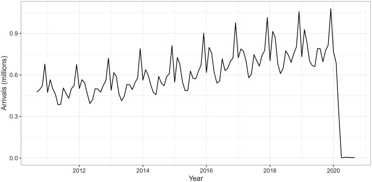
From a statistical modeling and forecasting perspective, these disruptions cause unique challenges. The pandemic has meant that we cannot extrapolate the strong and persistent signals observed in historical tourism time series. The structural break is deep and the path to recovery remains extremely uncertain. Figure 1 shows the latest data (at the time of writing) for Australia. It highlights the devastating effect on inbound travel with international arrivals dropping to around 3,000 passengers per month (all Australian nationals returning to Australia) beginning from April 2020, down from a peak of 1.1 million international travelers in December 2019.

Figure 1.

Short-term international arrivals to Australia up to September 2020.

Similar situations have been witnessed around the world (e.g., Airports Council International (ACI) Europe 2020; Richter 2020). Unlike many previous well-studied disruptions to tourism (for a comprehensive list see Bausch, Gartner, and Ortanderl 2021), the COVID-19 pandemic has caused a simultaneous global disruption. This has meant that much of the existing literature on modeling and forecasting tourism demand is not applicable (see Song, Qiu, and Park 2019, for the latest review). Even the literature that involves judgment is of limited assistance (e.g., Lin, Goodwin, and Song 2014; Song, Gao, and Lin 2013) as it focuses on integrating statistical forecasts with judgment (Arvan et al. 2019; Petropoulos, Fildes, and Goodwin 2016). The aim is to complement statistical forecasts with the domain knowledge of experts via judgmental adjustments. However, at this stage the statistical signal for many components of tourism has been completely washed out.

With model-based forecasts, the generation of prediction intervals to account for the inherent uncertainty of forecasting is now a common practice. This is less so when domain knowledge is superimposed on model forecasts, or direct judgmental forecasts are generated. To account for this, in the literature the generation of scenarios has become an established approach (examples in the recent tourism literature include, Fotiadis, Polyzos, and Huan 2021; Kourentzes et al. 2021; Liu et al. 2021; Qiu et al. 2021; Zhang et al. 2021). Nonetheless, the scenarios do not capture the uncertainty of specific forecasts, but rather the uncertainty on the conditionals on which the forecasts are built; in the case of the COVID-19 pandemic that might be the speed of the roll-out of vaccination programs, or the emergence of new strains of the virus. The conditioned forecasts will remain uncertain, and therefore, generating probabilistic scenario forecasts is more informative and can lead to better decisions. This has been largely overlooked when adjusting model forecasts with domain knowledge.

To the best of our knowledge this paper is the first to generate probabilistic scenario-based judgmental forecasts. We use a large survey from diverse experts and stakeholders, proposing a novel methodology to produce forecasts. Using survey responses we generate scenario-based probabilistic forecasts for Australian tourism. We concentrate on the two largest sectors of the Australian tourism industry: international arrivals and domestic tourism flows. The survey responses come from tourism experts and stakeholders within the industry drawing on first-hand experience and knowledge. We have designed the survey in order to cover market segments that are of interest to the policy maker and are expected to show diverse behavior. The expectation is that the various segments of tourism will be affected differentially and will recover at different rates.

Using historical data up to the end of 2019, we generate counterfactual “COVID-free” forecasts. In order to generate coherent and robust forecasts we combine to the concepts of forecast combinations and forecast reconciliation. The accuracy of these forecasts is evaluated against historical data. These set a baseline expectation for what would have been had COVID-19 not occurred.

The remainder of the paper is structured as follows. Section 2 provides a detailed literature review on judgmental forecasting within and outside the field of tourism. Section 3 presents the proposed innovative statistical methodology for generating scenario-based judgmental probabilistic forecasts accounting for the onset of the COVID-19 pandemic; as well as methodology for producing robust counterfactual forecasts based on historical pre-COVID-19 data by combining the notions of forecast reconciliation and forecast combinations. Section 4 presents the experimental design, exploring historical data and generating and evaluating the robustness of COVID-free counterfactual forecasts. Section 5 presents details of the survey design, the survey participants and the detailed analysis of the results together with a post-survey real time evaluation. Some discussion and conclusions follow in Section 6.

Literature Review on Judgmental Forecasting

Judgmental forecasting is widely used when there is lack of reliable data to build quantitative models, or there is contextual information that is unaccounted for in models. Judgment can be used to produce forecasts directly, or adjust existing forecasts, with both approaches having received substantial attention in the literature see recent reviews of the area by Arvan et al. 2019; Perera et al. 2019). Given the context of the COVID-19 pandemic and its dramatic effect on tourism, we focus on direct judgmental forecasts, as there is very limited data to generate model-based forecasts (Kourentzes et al. 2021; Zhang et al. 2021). Our objective in this section is to provide an overview of judgmental forecasting approaches in the context of their usability to support our forecasting task. The reader is pointed to Lawrence et al. (2006) and Ord, Fildes, and Kourentzes (2017, Chapter 11) for details on the different methods.

There are several considerations in the generation of judgmental forecasts, such as the use of a single or multiple humans, the nature of the forecast that could be a point prediction, scenarios, intervals, or a probabilistic forecast, and the use of domain experts or not. Humans benefit from the ability to use unstructured domain knowledge, but at the same time suffer from various cognitive biases (Fildes et al. 2009). Relevant examples are the availability bias (overly rely on easily available or memorable information), the representativeness heuristic (matching to a previous similar observation, ignoring the frequency of occurrence), the anchoring bias (the forecaster “anchors” to an initial estimate and does not consider substantially different values, e.g., the last observation), the over-optimism or motivational biases (motivated to forecast toward a preferred state), and overconfidence in own forecasting abilities (Ord, Fildes, and Kourentzes 2017, 386). This makes the use of single forecasters for obtaining predictions problematic, with performance varying substantially, as well as being difficult to identify consistently well-performing forecasters (Schoemaker and Tetlock 2016). Instead, many judgmental forecasting methods rely on the use of multiple individuals, to counter both this inconsistency, but also attempt to negate judgmental biases.

When using a jury of experts, the literature suggests avoiding face-to-face interactions (Armstrong 2006), as influential individuals may herd forecasts to a particular preference. A structured approach to overcome this is the Delphi method (for details see Rowe 2007). The Delphi method organizes the process by asking a group of experts (who do not interact directly) to provide their forecasts. In contrast to many other methods, experts are asked to provide the reasoning behind their predictions. Together with the forecasts, these are collected, summarized, and communicated anonymously to the panel of experts, who are asked to revise their predictions in light of the new information. Kauko and Palmroos (2014) provide insights into how the experts converge to a consensus over different rounds, reporting changes toward a more accurate consensus, but with changes being relatively small in magnitude. This iterative process can be repeated until there is adequate convergence between the forecasts. Lin and Song (2015, and references therein) provide a review of the Delphi method in the tourism forecasting literature, reporting that it is one of the most popular judgmental forecasting methods. However, its usefulness for generating forecasts remains contentious. For example, Song, Gao, and Lin (2013) and Lin, Goodwin, and Song (2014) report that Delphi was beneficial for the accuracy of tourism forecasts, however, in these experiments participants were asked to adjust statistical forecasts. Kauko and Palmroos (2014) and Graefe and Armstrong (2011) provide evidence that the Delphi method did not result in significantly more accurate predictions than face-to-face meetings, although such findings often point to the weakness of the application, rather than of the method itself (Ord, Fildes, and Kourentzes 2017).

An alternative to the Delphi method is the use of the so-called prediction markets. With prediction markets participants are asked to trade “shares” that correspond to a particular forecast outcome. As the market develops, the favored outcome by the participants is revealed. Prediction markets can be described as emulating simplified stock-markets, and therefore participants have a strong incentive to be accurate (Miles 2008; Tziralis and Tatsiopoulos 2007). Armstrong (2008) contrast the Delphi method with prediction markets and suggests that the Delphi method has the advantages that the reasoning behind forecasts is revealed, increasing confidence and that it can provide quicker predictions.

Notwithstanding, in both cases, as well as with the jury of experts, the selection of the participants is crucial. This relates to both the number of participants, as well as their domain knowledge. Tetlock (2017) provides multiple examples where experts have been unable to forecast major events. Ord, Fildes, and Kourentzes (2017) argue that experts may not represent a wide enough sample, quoting examples from the UK Brexit vote, but also because experts may operate on a similarly incomplete set of information. O’Leary (2017) investigates the accuracy of the wisdom of the crowd, going beyond experts, finding that a broad group of participants has a positive effect on accuracy. Petropoulos et al. (2018) find that the wisdom of the crowd can outperform statistical methods in identifying the best forecast, and although both generic crowds and domain experts performed well, the latter could achieve better performance with smaller groups of participants.

The literature has explored extensively the elicitation of the uncertainty in judgmental forecasts, or equivalently generating probabilistic judgmental forecasts (Lawrence et al. 2006). This task can take many forms, such as asking participants to provide probabilities to events, probabilities to specific values, provide prediction intervals, and so on. Although there is no consensus, the majority of the literature suggests that such forecasts suffer from overconfidence (see extensive discussion by Lawrence et al. 2006). The task format appears to affect the level of overconfidence, with a higher tendency when the forecaster has to assign probabilities to pre-selected values (Ronis and Yates 1987). Schoemaker (2004) connects overconfidence to psychological factors, such as the feeling of control, information distortions, and challenges in weighting probabilities. Kahneman and Lovallo (1993) suggest that forecasters who double as decision-makers often are influenced by their stakes in the decision, resulting in overly optimistic and confident predictions. We take this as a further argument in using a larger and wider group of forecasters. Interestingly increasing the information content of the task is correlated with overconfidence (Davis, Lohse, and Kottemann 1994), a finding that has many parallels with the arguments of Fildes, Goodwin, and Önkal (2019), who also find that forecasters act on information without being able to correctly assess its relevance to the task. Furthermore, Goodwin et al. (2019) show that when contrasting scenarios are offered as context, then forecasters’ confidence increases. Another interpretation of overconfidence for probabilistic forecasts is offered by Jørgensen and Sjøberg (2003) suggesting that when a point forecast is available forecasters anchor to it. The expertise of the forecasters does not seem to provide a consistent connection with performance (Lawrence et al. 2006). There is limited evidence that when asking participants to assign values to optimistic and pessimistic projections these correspond to extremes of the predictive distribution (5% and 95% respectively, Ord, Fildes, and Kourentzes 2017, 403).

The literature has explored ways to support the generation of judgmental forecasts. Decomposition aims to do that by breaking the task into smaller sub-tasks (MacGregor 2001). These sub-tasks are not only simpler to resolve, but further permit controlling the flow of information to reduce cognitive overload, as well as potential overconfidence. Edmundson (1990) finds that breaking a forecast in its constituents (e.g., trend, season) increased accuracy over providing a holistic forecast. Petropoulos et al. (2018) conclude the same effect when asking participants to identify the best forecast. Webby, O’Connor, and Edmundson (2005) observe the same when tasking forecasters to predict special events with different effects acting simultaneously. Tackling each effect separately increased the accuracy of the forecasts. Nonetheless, Goodwin and Wright (1993) warn that excessive decomposition may lengthen the task to the extent that mental fatigue may have adverse effects.

Similarly, in a judgmental forecasting task asking for very detailed or numerous estimates can degrade the accuracy of the forecasts (Miller et al. 2011; Ord, Fildes, and Kourentzes 2017). Therefore, care must be taken in the design of the task, so as to not overload the participants. Cook (2006) suggests structuring knowledge into schemas and increasing the working memory capacity by using both visual and verbal information as other ways to reduce cognitive load, the first, aligning well with the findings from the decomposition literature.

Focusing on the specific task, of predicting the effect of COVID-19 on tourism, we note that there have been numerous papers that advocate the use of judgment. Zhang et al. (2021) use the Delphi method to identify the expected decrease due to COVID-19 and the period when tourist arrivals will return to the baseline period, for three scenarios: pessimistic, normal, optimistic. By interpolating between these two points they construct weights with which they adjust econometric forecasts to reflect the impact of the pandemic. Qiu et al. (2021) construct three judgmental scenarios following a structured approach with no external experts. They use scenario projections from the United Nations World Tourism Organization to obtain the projected recoveries and linearly interpolate from observations at the onset of the pandemic. The linear interpolation is further enhanced by superimposing seasonality extracted through decomposition from the pre-pandemic data. Liu et al. (2021) use the Delphi method to obtain a judgmental index with two major components, the accessibility risk and the self-protecting measures, decomposing the predictive problem. These are then combined into a single index that is judgementally translated into adjustments for statistical forecasts. Finally, Kourentzes et al. (2021) rely on a panel of forecasters to obtain recovery projections, which are used to adjust model forecasts. As they ask for forecasts for multiple periods and combinations of origin-destination countries, they simplify the task into forecasting a binary restricted-unrestricted traveling outcome. They also ask forecasters to provide a percentage of recovery for the unrestricted traveling case. Recognizing the difficulty of the forecasting task, they combine all judgmental forecasts to obtain the adjustment weights for the model predictions. Combinations of forecasts have been shown to be an effective way to reduce individual biases, and improve the accuracy of the final prediction (Lawrence et al. 2006; Ord, Fildes, and Kourentzes 2017), relying on a “wisdom of the crowd” approach (Petropoulos et al. 2018; Surowiecki 2004). Finally, we note that none of these studies provide probabilistic forecasts, but rather alternative point forecasts, matching three scenarios.

Methodology

As demonstrated in Figure 1 the effect of the COVID-19 pandemic is such that historical data cannot be used to project forward without explicitly accounting for the depth and the length of the structural break caused by COVID-19, and the subsequent unknown and unprecedented path to recovery. Both the depth and length of the effect of the pandemic are extremely challenging or even impossible to estimate and predict statistically, and therefore we revert to a novel approach of judgmental forecasting. In this section we describe the methodology used to generate the post-COVID-19 scenario-based probabilistic forecasts and also the methodology implemented to generate counterfactual COVID-19-free forecasts which set the expected future paths had the pandemic never occurred.

Scenario-Based Probabilistic Forecasts Post-COVID-19

In order to generate scenario-based probabilistic forecasts, we survey tourism experts and stakeholders asking them to provide judgment on the future of tourism based on two types of questions. The first focuses on the level of tourism flows post-COVID-19 while the second focuses on the timing of the recovery to pre-COVID-19 levels.

• Question Type I: What will the level of tourism be at some point in time in the future, that is, 2021 Q4, compared to last observed flows prior to the COVID-19 pandemic, 2019 Q4.

Each respondent is asked to provide a high probability “Most likely” scenario, as well as low probability “Pessimistic” and “Optimistic” scenarios. The respondents are asked to choose form the categories shown in the left column of Table 1. We convert the discrete categories for each question into the scaling factors shown in the right column of the same table, using the midpoint of each range. For example, a response of “Lower 90–100%” means that the respondent expects that international arrivals in 2021 Q4 will be between 90% and 100% lower than they were in 2019 Q4. We convert this to the midpoint of “95% lower,” or equivalently at 5% of what they were in 2019 Q4 giving a scaling factor of 0.05.

Table 1.

Scaling Factors to Convert Survey Scenario Categorical Responses to a Continuous Distribution.

Category	Factor
Lower 90%–100%	0.05
Lower 70%–90%	0.20
Lower 50%–70%	0.40
Lower 30%–50%	0.60
Lower 10%–30%	0.80
Lower 0%–10%	0.95
Higher 0%–10%	1.05
Higher 10%–30%	1.20
Higher 30%–50%	1.40
Higher than 50%	1.60

Reflecting these design choices to the literature, for each scenario we ask the participants to provide a choice without prior forecasts (e.g., some point forecast from a model), to avoid any anchoring bias. Participants have to respond for the three scenarios, forcing them to contrast the alternatives, therefore mitigating any implicit assumptions on the likelihood of a single prediction that can occur by mixing probabilities with scenarios. We do not ask participants to provide a specific value, but rather to select amongst options, once for each scenario. This is done to mitigate other biases, such as overoptimism and overconfidence that may push predictions to extreme values, but also to manage the cognitive load. Finally, we pool the responses from multiple participants, to offset individual biases, but also building on the benefits of combining different judgmental forecasts.

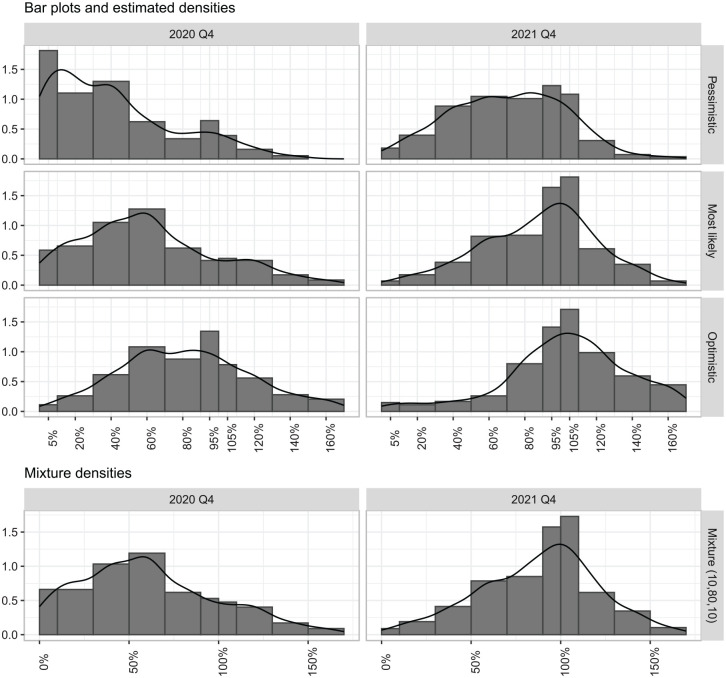
The top three rows of Figure 2 show bar plots and estimated probability densities of the responses for what the level of tourism flows be in 2021 Q4 compared to the last observed quarter of 2019 Q4. The example is based on Question 4 of the survey that follows and is used here for the purpose of demonstration (full details and analysis is presented in Section 5). The bar plots have been scaled to form probability densities, with the bar height adjusted according to the width of the corresponding interval and scaled to have area equal to 1.

Figure 2.

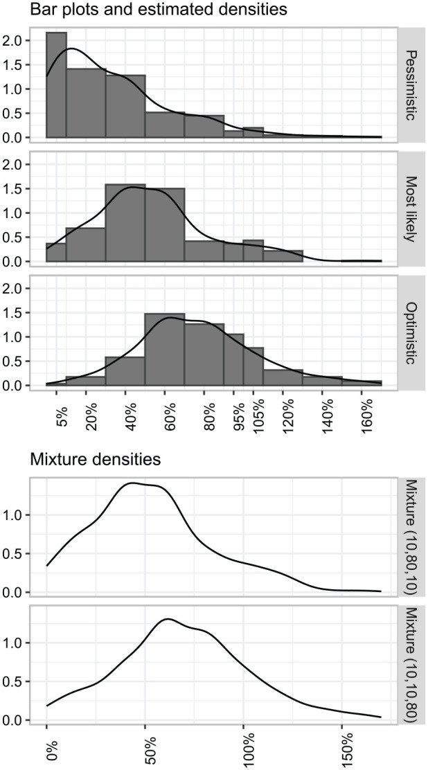
Scenario-based forecast distributions for international arrivals for 2021 Q4 compared to 2019 Q4, assuming international borders reopen in mid-2021. The horizontal scale represents the scaling factor applied to 2019 Q4 arrivals in order to estimate forecast distributions for 2021 Q4. The example is based on Question 4 of the survey.

This gives us a discrete probability distribution which is converted into a continuous distribution by summing zero-truncated Gaussian kernels (Jones 1993) placed at each point mass. We use a zero-truncated Gaussian kernel to ensure the distribution lies on the positive scale, to retain the probabilistic interpretation. The kernel density estimates (with bandwidth 0.1) are shown as the lines in the first three panels of Figure 2. They effectively combine neighboring options to give a smooth density across all possible scaling factors.

We next combine the three scenarios to form a weighted mixture distribution, shown in the fourth row of Figure 2. The weights used to combine the three scenarios are 0.1, 0.8, and 0.1; that is, we give the “Most likely” scenario an 80% probability of occurring and just 10% each for the other two highly unlikely scenarios. Combining the three scenarios using a mixture distribution accounts for both the uncertainty across the respondents and across each scenario, further offsetting individual biases.¹ Furthermore, the resulting mixtures help to simplify the communication of results and information to policy makers. These weights are not trained on data, but rather set by the users and policy makers, reflecting their propensity to risk. Similarly, as new information becomes available, this may alter their risk perceptions and result in updated weights. The aforementioned weights are illustrative, and arguably reflect the authors’ perceptions.

Our approach also allows a policy maker to weigh the scenarios asymmetrically as the circumstances change going forward. For example, as vaccinations progress, we can place more weight on the “Optimistic” scenario by setting the weights to 0.1, 0.1, 0.8 for “Pessimistic,” “Most likely,” and “Optimistic” scenarios respectively. The resulting mixture is shown in the fifth row of Figure 2.

In the last step of our method, we multiply the last pre-COVID-19 observation, 2019 Q4, with the estimated scaling factor density to obtain probabilistic scenario-based forecasts.

• Question Type II: What year do you think the level of tourism flows will return to pre-COVID-19 levels?

Again the respondents are asked to provide a high probability “Most likely” scenario, as well as low probability “Pessimistic” and “Optimistic” scenarios. The choice is set across the year range: 2021–2028. For this question type the discrete probability distribution based on years selected by the respondents is directly converted into a continuous distribution for the year of recovery by summing Gaussian kernels placed at each point mass with the bandwidth set to 0.6. Figure 3 shows an example based on Question 5 (full details and analysis is presented in Section 5). The top three panels show the the raw responses and kernel density estimates. The two bottom rows show the estimated mixture distributions.

Figure 3.

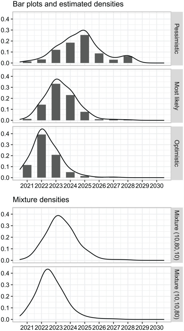
Scenario-based forecast distributions for the year international arrivals will recover to 2019 levels. The example is based on Question 5 of the survey.

COVID-Free Counterfactual Forecasts

Analyzing historical data gives us a good understanding of the trends and patterns within a tourism sector. Projecting them into the future reveals the expected future paths of tourism had the COVID-19 pandemic never occurred. Therefore it can be seen as what the tourism sector should possibly aspire to return to after the pandemic is over and the tourism industry has recovered. We label these as counterfactual “COVID-free” forecasts. Using counterfactual forecasts, policy makers can assess the difference between the judgmental scenarios that account for COVID-19 and the projections generated as if the pandemic had never occurred.

A commonly observed feature of tourism time series is that they form natural aggregation structures with attributes such as, geographic location and purpose of travel, that are of interest to policy makers and tourism operators. Cross-products of such attributes form what are referred to as grouped-time series Hyndman and Athanasopoulos (2021, Chapter 11). Over the last decade the concept of forecast reconciliation has been developed with the aim of generating coherent forecasts for such structures, that is, forecasts that adhere to the aggregation constraints and therefore aggregate in a consistent manner as the data. The concept was first introduced and implemented by Hyndman et al. (2011) and Athanasopoulos, Ahmed, and Hyndman (2009) with tourism aggregation structures the centerpiece of the literature as it has developed. Besides achieving coherency, Panagiotelis et al. (2021) show theoretical advantages of the reconciled forecasts.

Within tourism forecasting, Athanasopoulos, Ahmed, and Hyndman (2009), Kourentzes and Athanasopoulos (2019), Wickramasuriya, Athanasopoulos, and Hyndman (2019), and Kourentzes et al. (2021) provide empirical evidence that forecast reconciliation improves forecast accuracy over: (i) forecasting without considering aggregation constraints, hence generating incoherent forecasts, and (ii) applying traditional approaches for forecasting aggregation structures such as bottom-up or top-down. In this paper we implement the MinT (Minimum Trace) optimal forecast reconciliation approach of Wickramasuriya, Athanasopoulos, and Hyndman (2019). Forecast reconciliation is implemented by linearly combining a set of incoherent forecasts referred to as base forecasts and denoted here by ${\widehat{y}}_{T+h}$, using

$${\tilde{y}}_{T+h}=SG{\widehat{y}}_{T+h},$$ (1)

where $G$ is a matrix that maps the base forecasts into the bottom-level of the aggregation structure, and $S$ is a summing matrix that sums these up using the aggregation constraints, to produce a set of coherent forecasts denoted by ${\tilde{y}}_{T+h}$. For the optimal MinT approach

$$G=(S\prime W^{-1}S{)}^{-1}S\prime W^{-1}$$ (2)

where $W=\mathrm{Var}[(y_{T+h}-{\widehat{y}}_{T+h})]$ is the variance-covariance matrix of the base forecast errors and us estimated using a weighted least squares approximation, $\widehat{W}=\frac{1}{T}{\sum }_{t=1}^T{e}_t{e}_t^{\prime }$ where $e_t$ is a vector of residuals of the models that generated the base forecasts.

Furthermore, we use combinations of statistical forecasts to further enhance accuracy. Since the seminal work of Bates and Granger (1969) there has been a flurry of papers in implementing forecast combinations for improving accuracy over individual forecasts. There are two main arguments in favor of combining forecasts. First, it reduces the risk of selecting an inappropriate forecast, and second, it can improve forecast accuracy. There are several forecast combination methods, with simpler approaches often performing better (Barrow and Kourentzes 2016). Smith and Wallis (2009) and Claeskens et al. (2016) showed that this was largely due to the estimation uncertainty in the combination weights that are part of the more complex approaches. When there are only a few forecasts, simple combination operators, such as the mean or the median, perform very well, and increase the normality of forecast errors (Barrow and Kourentzes 2016). When more forecasts are available, forecast pooling can be advantageous, where first a smaller pool of forecasts is selected from all available forecasts, which are subsequently combined (Kourentzes, Barrow, and Petropoulos 2019). This reduces the need for estimating combination weights, as well as filtering potentially damaging forecasts.

Forecast combination shares a lot of principles with the “wisdom of the crowd” that is often employed in generating judgmental estimates (Petropoulos et al. 2018). There is ample empirical evidence of the performance of forecast combination, such as Montero-Manso et al. (2020) and Petropoulos and Svetunkov (2020), being among the top performing methods in large scale forecasting competitions, such as the M4 (see Makridakis, Spiliotis, and Assimakopoulos 2020). Forecast combination has also been prominent within the tourism literature. For example, Wong et al. (2007), Shen, Li, and Song (2008), Song et al. (2009), Shen, Li, and Song (2011), Li et al. (2019), and Qiu et al. (2021) provide evidence of the benefits of forecast combination in tourism forecasting.

With the above features in mind we generate base forecasts for each times series within each aggregation structure from ARIMA and ETS (exponential smoothing) models, automatically selected in the fable package (O’Hara-Wild, Hyndman, and Wang 2020) using the AICc, and also a combination (the average) of the two. We then reconcile forecasts across each structure to generate coherent forecasts, that is, point and probabilistic forecasts, using the WLS estimator in the Wickramasuriya, Athanasopoulos, and Hyndman (2019) optimal MinT (minimum trace) forecast reconciliation approach. Further, details of the processes used here are available in Hyndman and Athanasopoulos (2021, Chapter 11).

Experimental Design: Sectors, Historical Data, Counterfactual Forecasts, and Evaluation

We focus on the two largest sectors of Australian tourism namely international arrivals and domestic flows (the third one being outbound travel). Table 2 shows the details of grouped aggregation structures for the time series of each sector. For international arrivals we consider six international “Regions” crossed with five purposes of travel, while for domestic flows there are eight Australian states and territories crossed with four purposes of travel. These lead to a total of 42 and 45 series respectively that follow grouped aggregation structures with 30 and 32 series at the bottom-levels as a result of the two-way interactions between Region and Purpose for international arrivals, and State and Purpose for domestic visitor nights.

Table 2.

Grouped Structures for International Arrivals and Domestic Visitor Nights.

Grouping	No. of series	Grouping	No. of series
International arrivals		Domestic visitor nights
Total aggregate	1	Total aggregate	1
Region	6	States	8
Purpose	5	Purpose	4
Region × Purpose	30	States × Purpose	32

International Arrivals

International arrivals data span the period 2005 Q1–2019 Q4 and include all arrivals to Australia. The source of this data is the Australian Bureau of Statistics (ABS) Catalog 3401.0 covering overseas arrivals and departures data. The left column in Table 3 shows the nineteen source countries considered. To facilitate the judgmental predictions, these are aggregated into six international “Regions” of interest to the Australian tourism industry shown in the right column. Also of interest is the “Purpose” of travel, as traveler behavior and the impact of COVID-19 will vary across different purposes of travel. The purposes of travel for international arrivals to Australia are categorized as “Holiday,” “VFR” (visiting friends are relatives), “Education,” “Business,” and “Other.”

Table 3.

Source Countries and Regions for Australian International Arrivals.

Country	Region
China	China
Hong Kong	Other Asia
Thailand
Malaysia
Indonesia
Singapore
Japan
South Korea
India
Other Asia
United Kingdom	Europe
Germany
France
Other Europe
New Zealand	New Zealand
United States	The Americas
Canada
Middle East	Other World
Other World

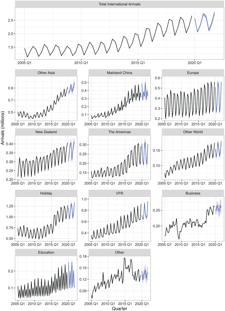
The quarterly time series for the overall aggregate, and the aggregates for regions and purposes of travel are shown in Figure 4, together with counterfactual forecasts, generated by the process described in Section 3.2. Some interesting and important observations emerge. International arrivals to Australia show a strong and consistent positive trend over the last few years. This is captured and projected in the counterfactual forecasts. An anomaly appears in the “Business” and “Other” series; there seems to be a direct substitution or redefinition between “Business” and “Other” travel in 2017 Q2, with an abrupt upward shift in the former matched by a downturn shift of equal size in the latter, possibly related to changes in visa entry rules to Australia in 2017.

Figure 4.

Time series and counterfactual COVID-free forecasts for 2020–2021 for total international arrivals to Australia, and the same data disaggregated by state and by purpose of travel. The shaded regions correspond to 95% prediction intervals.

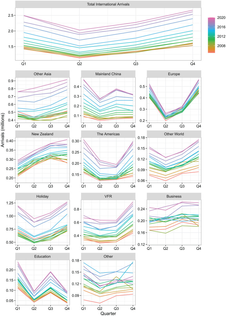
All arrivals also display a strong seasonal component which is reflected in the counterfactual forecasts. In almost all cases, this component appears to be multiplicative in nature, so that seasonal deviations increase proportionally to the increasing level of the series. Figure 5 is a seasonal plot (Hyndman and Athanasopoulos 2021) providing a more detailed view of the seasonal patterns. “Holiday” and “VFR” seem to be the main drivers of the seasonality in the aggregate series as well as for “The Americas,” Europe, and the “Other World” series. For these series, peaks are observed in Q1 and Q4, which include the summer period in Australia. In contrast, the “Education” series shows peaks in Q1 and Q3 corresponding to the beginning and the mid-point of the academic year in Australia. This seems to be the main source driving arrivals from Mainland China. One region showing asynchronous seasonality with the rest of the world is New Zealand with troughs in Q1 and peaks in Q3. Note the importance of considering these at the disaggregate level and implementing forecast reconciliation, as these country based and purpose specific features are lost at the aggregate level.

Figure 5.

Seasonal plots of total international arrivals to Australia, and the same data disaggregated by region and by purpose of travel.

Domestic Visitor Nights

We consider “visitor nights” across Australia as a measure of domestic tourism flows. The data are provided by the National Visitor Survey based on an annual sample of 120,000 Australian residents aged 15 years and older. The way the data is collected has developed over the years, switching at the beginning of 2014 from telephone interviews to a 50:50 mobile/landline split. The sample spans the period 1998 Q1–2019 Q4. We disaggregate these into the eight Australian states and territories, and four purposes of travel.

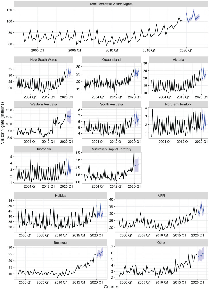
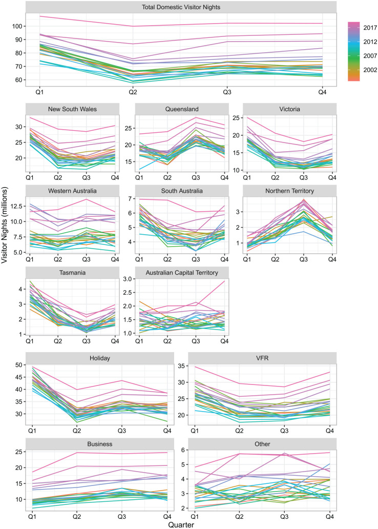
Figure 6 shows time plots and counterfactual forecasts for the aggregate, across each of the states and territories and for each purpose of travel. The states show positive consistent trends since 2012, and these are reflected in the counterfactual forecasts. There appear to be some structural breaks in the series for the Northern Territory and Western Australia, perhaps due to changing definitions or data recording practices. All series by purpose of travel also show significant positive trends over the last few years. The seasonal plots in Figure 7 highlight the differences in the northern states, such as Queensland and the Northern Territory and southern states, such as New South Wales, Victoria, South Australia, and Tasmania. The peak visits for the former occur in winter (corresponding to Q3) due to the tropical climate and rainy summer months while for the latter the peak is in summer (corresponding to Q1).

Figure 6.

Time series and counterfactual COVID-free forecasts for 2020–2021 for total Australian domestic visitor nights, and the same data disaggregated by state and by purpose of travel. The shaded regions correspond to 95% prediction intervals.

Figure 7.

Seasonal plots of total Australian domestic visitor nights, and the same data disaggregated by state and by purpose of travel.

Out-of-Sample Forecast Evaluation

Withholding the last two years of data, 2018 Q1–2019 Q4, across all the series as a test-set, we generate 1- to 8-steps-ahead forecasts and evaluate their accuracy against the actual observations of the test-set. Table 4 shows the MAPE (mean absolute percentage error), MASE (mean absolute squared error) and RMSSE (root mean squared scaled error) calculated over the test-sets across all the series for each of the international and domestic grouped structures (see Section 5.8 in Hyndman and Athanasopoulos 2021, for detailed definitions of these forecast error measures). The results show that for both structures the combined and reconciled forecasts are the most accurate. That is, the process of first combining ARIMA and ETS forecasts, to generate incoherent base forecasts, and then using MinT to optimally reconcile these, results to the most accurate pre-COVID-19 forecasts.

Table 4.

1 to 8-Steps Ahead Out-of-Sample Forecast Accuracy Evaluation Over the Test-Set Period 2018Q1–2019 Q4 for Australian International Arrivals and Domestic Visitor Nights.

Model	International arrivals			Domestic visitor nights
	MAPE	MASE	RMSSE	MAPE	MASE	RMSSE
ARIMA	10.93	1.38	1.17	21.98	1.74	1.59
ETS	8.16	1.16	1.05	21.38	1.69	1.54
Combined	8.62	1.12	0.99	21.38	1.68	1.53
Combined and reconciled	8.21	1.07	0.93	20.80	1.65	1.52

A note on the evaluation

The purpose of Table 4 is to allow for the comparison of forecast accuracy between methods within each structure and not to compare across the two structures. However, there is an obvious drop in forecast accuracy between international arrivals and domestic visitor nights, although it is worth reiterating that the rankings between methods within each structure remain consistent. Such anomalies are always worth investigating. Figures S1 and S2 in Supplemental Appendix A present point and interval forecasts as well as the actual values for the test-period 2018 Q1–2019 Q4, for international arrivals and domestic flows respectively.

Visual inspection indicates that the forecasts perform remarkably well in capturing the movements in the international arrivals test-set data. In contrast, for many of the domestic series, there seems to be a very strong and sudden increase in the trend during the test-set period with not enough history provided for the models to capture this. The sudden increase can be seen in the aggregate series and also throughout the various components. This highlights the relatively lower accuracy of the domestic forecasts over the test-set compared to the international arrivals. We note that with another two years of history, this trend correction has been captured by the models and is included in the counterfactual forecasts as shown in Figure 6.

Results

Survey Design and Participants

In order to generate scenario-based probabilistic forecasts, we surveyed tourism experts and stakeholders asking them to provide judgment on the future of both international arrivals to Australia and domestic visitor nights. The survey took place in September 2020 and there were 443 participants with valid responses.

We sought a wide participation, as this is beneficial for judgmental forecasts, both in terms of sample to counterbalance biases and for incorporating viewpoints from multiple sectors and stakeholders. The latter is important to include a wide variety of perspectives, so as to avoid relying on a small sample of experts and stakeholders who may have a similarly biased viewpoint. The survey comprised of only eleven questions ensuring that it was engaging and manageable for participants. In the following sections we summarize and analyze the key results. The complete survey design and questionnaire is presented in Supplemental Appendix B. The descriptive analysis in this section shows the diversity of the respondents in terms of: sector, size of organization and the direct effect of the COVID-19 pandemic has had on their organization.

• Question 1: Which sector best describes your organization?

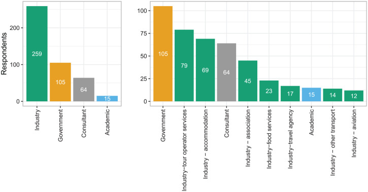
The sector distribution from which the participants came is shown in Figure 8. The left panel shows that the largest proportion of participants came from “Industry,” followed by “Government.” The breakdown within each sector is shown in the right panel.

Figure 8.

Which sector best describes your organization?

• Question 2: How many people are currently employed by your organization ?

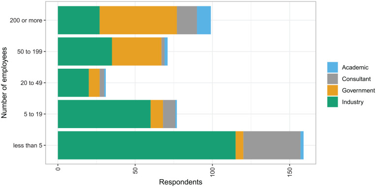
Figure 9 shows the size distribution of employer organizations for the respondents. Small industry businesses are well represented in the sample as well as larger government organizations.

Figure 9.

How many people are currently employed by your organization?

• Question 3: How does this employment figure compare with the start of 2020?

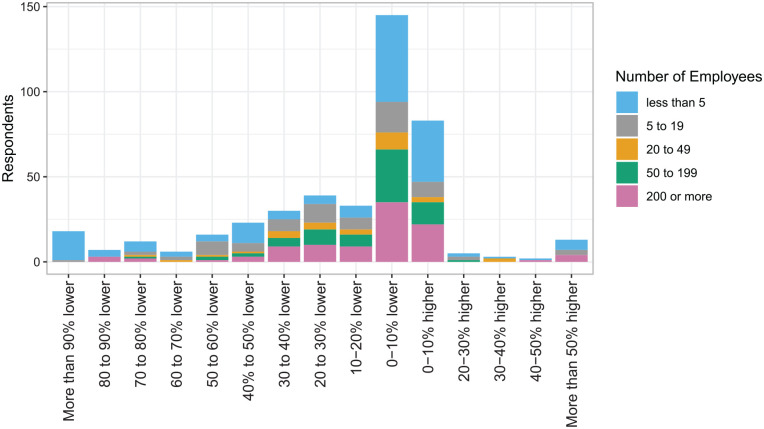
Figure 10 shows the change in the numbers employed in the organizations compared to the beginning of 2020, hence just pre-COVID-19. The top panel shows the distributions collectively. The most common response seems to be a 0%–10% decrease followed by a 0%–10% increase. Hence, overall it is most common to observe a change of up to 10% in absolute value. However, there is a long left tail to this distribution with mostly small businesses (fewer than 20 employees) taking the biggest hit. The bottom panels break this down by sector and shows that most of the decreases come from organizations labeled as “Industry” or “Consultant,” with the “Government” sector not being significantly affected outside the 10% change range.

Figure 10.

How does the number of people employed in your organization compare with the start of 2020?

Scenario-Based Probabilistic Forecasts for International Arrivals

In this section we present the results and detailed analysis for Questions 4–7 related to international arrivals to Australia.

• Question 4: What will the level of international arrivals to Australia be in 2021 Q4 compared to 2019 Q4?

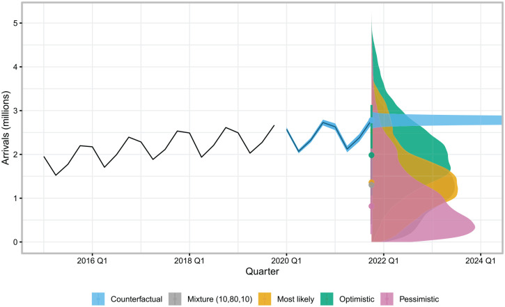
Implementing the methodology of Section 3, results to the scenario-based forecast distributions together with the path and the distributions of the COVID-free counterfactual forecasts, plotted in Figure 11. This plot provides a good understanding of the locations of the distributions relative to the counterfactual forecasts and the last observed value, as well as an excellent visual on the differences between the distributions. Note that we drop the “Mixture (10,10,80)” from all figures to avoid congesting the plots. The counterfactual forecast distribution has been truncated in order to assist with visualization. The figure also highlights the substantial difference in the uncertainty between the scenario-based forecasts under COVID-19 and the counterfactual COVID-free forecasts for 2021 Q4.

Figure 11.

Scenario-based and counterfactual COVID-free forecast distributions for international arrivals to Australia for 2021 Q4. Note that the counterfactual forecast distribution has been truncated in order to assist with visualization.

Some specific statistics of interest are presented in Table 5. By comparison, the value of 2019 Q4, the last pre-COVID-19 quarter, is 2.67 million arrivals. Under the “Mixture (10,80,10)” distribution, the median forecast value for 2021 Q4 shows 1.30 million arrivals. This is a predicted decrease of 51% compared to 2019 Q4, instead of a 4% increase shown by the counterfactual COVID-free forecast value. The 80% prediction interval for the same “Mixture (10,80,10)” distribution scenario returns a range for the decrease in international arrivals between 8% and 85%. The width of the prediction interval further highlights the tremendous uncertainty of the future of international arrivals after the COVID-19 pandemic has hit, compared to the tightness of the counterfactual COVID-free 80% prediction interval which shows an increase between 2% and 7%.

Table 5.

Scenario-Based and Counterfactual COVID-Free Forecasts for International Arrivals to Australia in (Millions) for 2021 Q4. The Observed Value for 2019 Q4 is 2.67.

Scenario	Mean	Median	80%	95%
Counterfactual	2.78	2.78	[2.72, 2.85]	[2.68, 2.88]
Pessimistic	1.00	0.82	[0.18, 2.13]	[0.05, 2.97]
Most likely	1.45	1.36	[0.51, 2.59]	[0.18, 3.24]
Optimistic	2.05	1.98	[1.07, 3.13]	[0.56, 3.91]
Mixture (10,80,10)	1.37	1.30	[0.40, 2.46]	[0.13, 3.07]
Mixture (10,10,80)	1.70	1.69	[0.44, 2.84]	[0.12, 3.52]

• Question 5: In what year do you think international visitor numbers will return to 2019 levels?

Figure 12 shows the raw responses, kernel density estimates (bandwidth 0.6), and the estimated mixture distributions for when respondents anticipate international arrivals to recover to 2019 Q4 levels. The bottom panel plots the estimated forecast distributions superimposed on each other across the time axis for international arrivals. The plot shows the contrasts between the distributions for the different scenarios as the peak of the estimated densities moves further into the future as the scenario moves from “Optimistic” to “Most likely” to “Pessimistic.” Table 6 shows some specific statistics of interest. The median recovery quarter varies from 2022 Q3 in the “Optimistic” scenario to 2025 Q1 in the “Pessimistic” scenario. The median recovery quarter for the “Mixture (10,80,10)” distribution is 2023 Q4 with the 80% prediction interval showing as lower bound 2022 Q2 and upper bound 2025 Q2.

Figure 12.

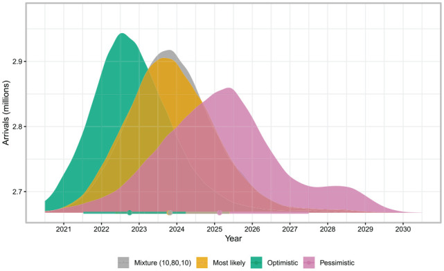
Forecast distributions of when international arrivals will recover to 2019 levels estimated from survey responses to Question 5.

Table 6.

Recovery Scenarios for International Arrivals.

Scenario	Mean	Median	80%	95%
Pessimistic	2025 Q1	2025 Q1	[2023 Q1, 2027 Q3]	[2022 Q1, 2028 Q4]
Most likely	2023 Q4	2023 Q4	[2022 Q2, 2025 Q2]	[2021 Q3, 2026 Q3]
Optimistic	2022 Q4	2022 Q3	[2021 Q3, 2024 Q1]	[2020 Q4, 2025 Q2]
Mixture (10,80,10)	2023 Q4	2023 Q4	[2022 Q2, 2025 Q2]	[2021 Q3, 2026 Q2]

• Questions 6 and 7: In what year do you think international visitor numbers for the following markets will return to 2019 levels? Please provide estimates only for the most likely scenario.

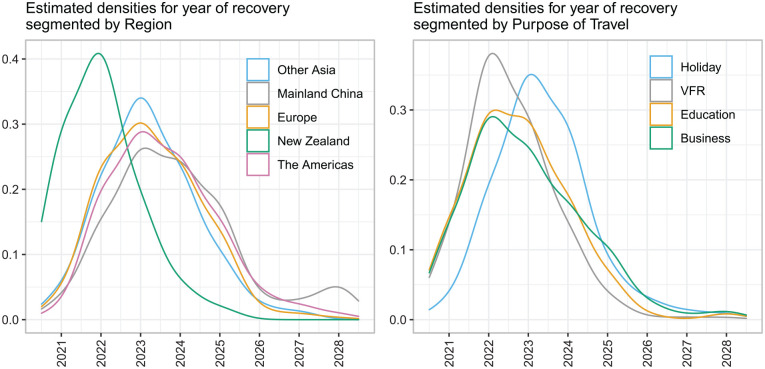
In order to keep the respondents engaged and the survey manageable, respondents were required to provide estimates only for the “Most likely” scenario for the markets segmented by the five international “Regions” as shown in Table 3 and for the “Purposes” of travel. The bar plots of the raw responses and fitted kernel density estimates (bandwidth = 0.5) are presented in Figure 13. Table 7 shows some specific statistics of interest. The results show that the respondents have selected New Zealand as the international arrivals source that will recover the quickest with median predicted quarter of full recovery 2022 Q2. Mainland China is selected to be the slowest to recover, with median predicted quarter of full recovery 2024 Q1. In terms of purpose of travel the results show that “Holiday” travel will be the slowest to recover with median predicted quarter of full recovery 2023 Q4, with “VFR” the quickest to recover with median predicted quarter of full recovery 2022 Q4 of course, there is high uncertainty surrounding these point predictions as indicated by the width and the asymmetry of the prediction intervals with most distributions showing a very long right tail.

Figure 13.

Estimated densities for the most likely year international visitor numbers will return to 2019 levels for Regions and for Purpose of Travel.

Table 7.

Recovery Scenarios for International Markets.

	Mean	Median	80%	95%
International regions
Other Asia	2023 Q3	2023 Q3	[2022 Q1, 2025 Q2]	[2021 Q2, 2026 Q3]
Mainland China	2024 Q2	2024 Q1	[2022 Q2, 2026 Q3]	[2021 Q3, 2028 Q3]
Europe	2023 Q4	2023 Q3	[2022 Q1, 2025 Q3]	[2021 Q2, 2026 Q3]
New Zealand	2022 Q3	2022 Q2	[2021 Q1, 2024 Q1]	[2020 Q3, 2025 Q1]
The Americas	2024 Q1	2023 Q4	[2022 Q2, 2025 Q4]	[2021 Q3, 2027 Q2]
Purpose of travel
Holiday	2023 Q4	2023 Q4	[2022 Q2, 2025 Q3]	[2021 Q3, 2027 Q1]
VFR	2023 Q1	2022 Q4	[2021 Q3, 2024 Q3]	[2020 Q4, 2025 Q3]
Business	2023 Q2	2023 Q2	[2021 Q3, 2025 Q3]	[2020 Q4, 2026 Q4]
Education	2023 Q2	2023 Q1	[2021 Q3, 2025 Q1]	[2020 Q4, 2026 Q1]

Scenario-Based Probabilistic Forecasts for Domestic Visitor Nights

In this section we present the results for Australian domestic visitor nights. In contrast to international arrivals respondents were asked to provide scenarios for both 2020 Q4 as well as 2021 Q4.

• Question 8: What will the level of domestic visitor nights be in 2020 Q4 and 2021 Q4 compared to 2019 Q4?

The left column of Figure 14 shows bar plots and estimated densities for the survey responses for 2020 Q4 while the results for 2021 Q4 are shown in the right column. The rows summarize the results for the “Pessimistic,” “Most likely” and “Optimistic” scenarios as well as the “Mixture (10,80,10)” distribution. The peak of the “Mixture (10,80,10)” distribution shows approximately 50% of the domestic visitor nights will be maintained for 2020 Q4 compared to 2019 Q4, while moving closer to full recovery for 2021 Q4.

Figure 14.

Scenarios for domestic visitor nights for 2020 Q4 and 2021 Q4 compared to 2019 Q4. The x-scale for the fitted densities represents the scaling factor applied to domestic flow counts of 2019 Q4 in order to estimate forecast distributions for 2020 Q4 and 2021 Q4.

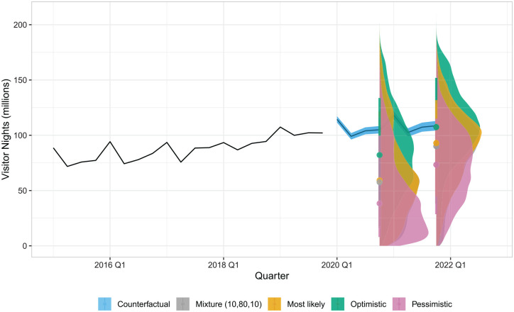
The scenario-based forecast distributions as well as the paths and prediction intervals for the counterfactual COVID-free forecasts are shown in Figure 15. All scenarios show a substantial decrease compared to the counterfactual forecasts for both 2020 Q4 and 2021 Q4, with the exception of the “Optimistic” scenario for 2021 Q4. The shapes of the forecast distributions reflect the tremendous uncertainty surrounding domestic tourism due to the COVID-19 pandemic when compared to the COVID-free counterfactual forecast distributions.

Figure 15.

Scenario-based and COVID-free counterfactual forecast distributions for Australia domestic visitor nights for 2020 Q4 and 2021 Q4.

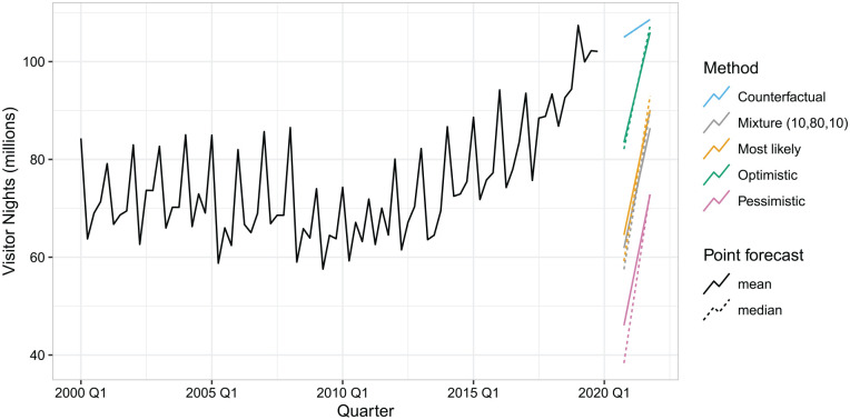
Figure 16 provides insights on the projections of the scenario based forecasts between the two years. The plot shows that the trends (both means and medians) projected between 2020 Q4 and 2021 Q4 are fairly consistent across the three scenarios and the mixture. It also shows the higher growth between the two years across all scenarios compared to the growth shown for the counterfactual COVID-free forecasts, anticipating a faster rate of recovery.

Figure 16.

Paths of projections for domestic visitor nights showing consistency in respondents.

Table 8 provides some specific statistics of interest. The median forecasts for the “Mixture” distribution are 57.3 and 89.8 million visitor nights for 2020 Q4 and 2021 Q4 respectively. These show a decrease of 44% and 12% compared to projected increases of % and % for the counterfactual COVID-free forecasts. Hence, the expectation for domestic tourism seems to be that after the deep hit of 2020, there will be a rapid recovery for 2021 although one should always keep in mind the considerable width of the prediction intervals. Specifically, the 80% interval for the “Mixture” distribution shows decreases ranging between 84% and 14% for 2020 Q4. For 2021 Q4, the lower bound shows a decrease of 62% while the upper bound an increase by 25%.

Table 8.

Scenario-Based and Counterfactual COVID-Free Forecasts for Australian Domestic Visitor Nights in (Millions) for 2020 Q4 and 2021 Q4. The Observed Value for 2019 Q4 is 102.09.

Quarter	Scenario	Mean	Median	80%	95%
2020 Q4	Counterfactual	104.99	104.99	[102.80, 107.19]	[101.64, 108.35]
2020 Q4	Pessimistic	46.08	38.35	[7.96, 99.69]	[2.23, 125.06]
2020 Q4	Most likely	64.55	59.20	[17.50, 121.52]	[5.54, 149.23]
2020 Q4	Optimistic	83.46	82.11	[35.68, 133.70]	[15.09, 161.49]
2020 Q4	Mixture (10,80,10)	61.88	57.53	[15.99, 116.43]	[5.26, 144.44]
2021 Q4	Counterfactual	108.61	108.61	[105.78, 111.44]	[104.28, 112.94]
2021 Q4	Pessimistic	72.85	73.35	[28.59, 114.90]	[11.49, 135.82]
2021 Q4	Most likely	90.11	92.99	[44.91, 131.55]	[20.32, 152.31]
2021 Q4	Optimistic	105.99	107.38	[61.14, 151.90]	[20.48, 169.30]
2021 Q4	Mixture (10,80,10)	86.41	90.03	[38.27, 128.34]	[11.72, 148.30]

• Question 9: In what year do you think domestic visitor nights will return to 2019 levels?

Figure 17 shows the bar plots, kernel density estimates and superimposed forecast distributions for when respondents anticipate domestic visitor nights to recover to 2019 Q4 pre-COVID-19 levels. The plot shows the contrasts between the distributions for the different scenarios as the peak of the estimated densities moves further into the future as the scenario moves from “Optimistic” to “Most Likely” to “Pessimistic.”

Figure 17.

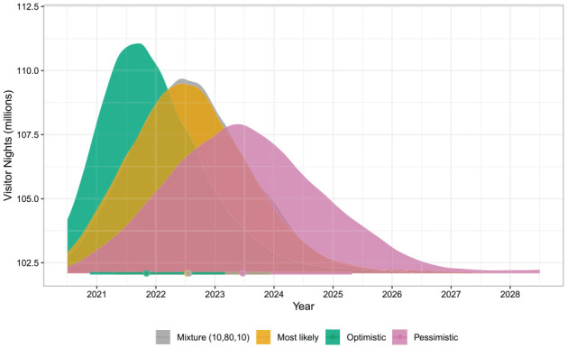
Scenarios for the year domestic visitor nights will recover to 2019 levels.

Table 9 shows some specific statistics of interest. The median recovery quarter varies from 2021 Q4 for the “Optimistic” scenario to 2023 Q2 for the “Pessimistic” scenario. The median recovery quarter for the “Mixture (10,80,10)” distribution is 2022 Q3 with the 80% prediction interval showing as lower bound 2021 Q2 and upper bound 2023 Q4.

Table 9.

Recovery Scenarios for Domestic Visitor Nights.

Scenario	Mean	Median	80%	95%
Pessimistic	2023 Q3	2023 Q2	[2021 Q4, 2025 Q2]	[2021 Q1, 2026 Q2]
Most likely	2022 Q3	2022 Q3	[2021 Q2, 2023 Q4]	[2020 Q3, 2024 Q4]
Optimistic	2021 Q4	2021 Q4	[2020 Q4, 2023 Q1]	[2020 Q2, 2024 Q1]
Mixture (10,80,10)	2022 Q3	2022 Q3	[2021 Q2, 2023 Q4]	[2020 Q4, 2024 Q4]

• Questions 10 and 11: In what year do you think domestic visitor nights will return to 2019 levels for the following markets?

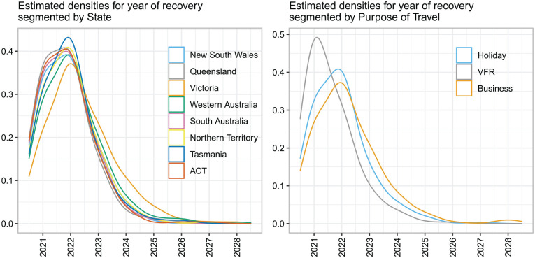
Similar to Questions 6 and 7, respondents were required to provide estimates only for the “Most likely” scenario for the markets segmented by “States” and “Purpose” of travel. The bar plots of the raw responses and fitted kernel density estimates are presented in Figure 18.

Figure 18.

Estimated densities for the most likely year that domestic visitor nights will return to 2019 levels for states and purpose of travel.

Table 10 shows some specific statistics of interest. The results do not show much variation across the states with the median expected quarter of full recovery to 2019 Q4 levels, being 2022 Q2. The only slight variations seems to be an anticipated earlier recovery by one quarter for Queensland, and a later recovery also by one quarter for Victoria. We should note that at the time of the survey being conducted Victoria was going through a second wave with severe lockdown measures and a night curfew in place.

Table 10.

Recovery Scenarios for Domestic Visitor Nights.

	Mean	Median	80%	95%
States
New South Wales	2022 Q2	2022 Q2	[2021 Q1, 2023 Q4]	[2020 Q3, 2024 Q3]
Queensland	2022 Q2	2022 Q1	[2021 Q1, 2023 Q3]	[2020 Q3, 2024 Q3]
Victoria	2022 Q4	2022 Q3	[2021 Q2, 2024 Q3]	[2020 Q4, 2025 Q4]
Western Australia	2022 Q3	2022 Q2	[2021 Q1, 2024 Q1]	[2020 Q3, 2025 Q2]
South Australia	2022 Q2	2022 Q2	[2021 Q1, 2023 Q3]	[2020 Q3, 2024 Q3]
Northern Territory	2022 Q2	2022 Q2	[2021 Q1, 2023 Q4]	[2020 Q3, 2024 Q4]
Tasmania	2022 Q2	2022 Q2	[2021 Q1, 2023 Q4]	[2020 Q3, 2024 Q4]
Australian Capital Territory	2022 Q2	2022 Q2	[2021 Q1, 2023 Q3]	[2020 Q3, 2024 Q3]
Purpose of travel
Holiday	2022 Q2	2022 Q2	[2021 Q1, 2023 Q4]	[2020 Q3, 2025 Q1]
VFR	2022 Q1	2021 Q4	[2020 Q4, 2023 Q2]	[2020 Q2, 2024 Q3]
Business	2022 Q3	2022 Q3	[2021 Q1, 2024 Q2]	[2020 Q3, 2025 Q4]

In terms of purpose of travel, the results show that VFR is anticipated to be the quickest to recover with median predicted quarter of full recovery 2021 Q4 followed by Holiday with median predicted quarter of recovery 2022 Q2. The slowest to recover is anticipated to be Business travel with median predicted quarter of full recovery 2022 Q3. Of course, the high uncertainty surrounding these point predictions is highlighted by the width and the asymmetry of the prediction intervals with most distributions showing a considerably long right tail.

A Post-Survey Real Time Evaluation

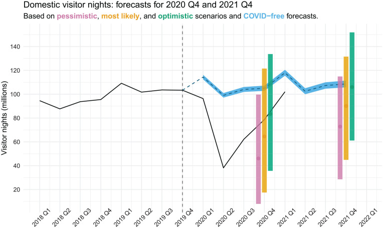
Upon completing the write up of the paper and with many developments related to COVID-19 pandemic, such as several vaccines being available around the world, we had the opportunity to evaluate the quality of our probabilistic scenario-based forecasts. We do this for Australian domestic tourism as the Australian international border remains closed to arrivals at the time of evaluation. Figure 19 shows the updated data for Australian domestic visitor nights, now including observations up to 2021 Q4. After reaching a low point of approximately 40 million in 2020 Q2, Australian domestic visitor nights increased to over 78.7 million in 2020 Q4. This value has been well captured by the 80% forecast intervals from all three scenarios, with the mean of the optimistic scenario being the closest and only 4.76 million above the observed value. This is a remarkable performance from the proposed methodology and provides solid evidence of the soundness and usefulness of the approach.

Figure 19.

A post-survey real time evaluation for Australian domestic visitor nights. The plot shows scenario-based judgmental forecasts from experts and stakeholders taking into account the COVID-19 pandemic as well as COVID-free statistical forecasts, plotted against data observed post the survey being completed. All forecast intervals are estimated to provide 80% coverage.

The second wave of the pandemic hit Australia during July–August 2020, with the majority of cases concentrated in the state of Victoria. With the tight controls, including strict and effective regional lockdowns by Australian state governments where they were deemed to be necessary, it seems that Australian domestic tourism was well on the road to recovery to pre-pandemic levels during the second half of 2020. Domestic visitor nights continued to increase to over 100 million in 2021 Q1, the summer quarter for Australia.

Discussion and Conclusions

The onset of the COVID-19 pandemic has been arguably the greatest challenge faced by the global community over the last few decades. The necessary efforts of nations to slow down the transmission of the virus has severely affected global tourism. Understanding how the sector may recover is key for policy makers, tourism planners and destination marketers, whether they are in government or in business. The depth and severity of the disruption has meant that forecasting practice “as usual” is no longer possible.

In this paper we have provided an innovative methodology to generate probabilistic forecasts for the path to recovery that can support policy and planning. Conducting a large scale survey we asked tourism experts and stakeholders to provide their judgment for three alternative scenarios: “Pessimistic,” “Most likely,” and “Optimistic.” Using their responses we built judgmental scenario-based probabilistic forecasts for numerous segments of the Australian tourism industry that are of interest to policy makers. The respondents anticipated different markets to be affected at different levels and to recover at different rates.

Our proposed approach can serve as a blueprint for generating similar forecasts for different countries and regions. We argue that the collection of data from participants is relatively easy, as we do not require the composition of an expert panel, which can be time-consuming and potentially expensive, but rather rely on the wide participation from various stakeholders and sectors. Our online survey was engaging and allowed us for a wide reach, as evident by the number of participants. This easiness of collecting views from a large number of participants mitigates judgmental biases, that may remain in smaller panels of experts, for instance by relying on the same sources of information. Nonetheless, with the increasing usefulness of online collection of judgmental estimates, future research should investigate the optimal design of such surveys for forecasting purposes.

Although human judgment is very useful for generating forecasts in situations where past historical observations are of little relevance, as is the case for the COVID-19 pandemic, we recognize that there are still weaknesses in the approach. We remedy these by, first, generating multiple probabilistic scenarios, and second, offering a way for decisions makers to weigh and mix these scenarios. On the one hand, the multiple probabilistic scenarios enable us to assess not only the different potential futures but also the uncertainty in each of these, as reflected in the shape of the distributions. On the other hand, the mixture result is robust in both reducing any estimation issues coming from the statistical treatment of the forecasts, but also in further mitigating any biases or misunderstandings by the participants. We argue that the last point is crucial. There is evidence in the literature that humans can obfuscate the generation of scenarios with the extremes of probabilistic forecasts, as discussed in Section 2. By asking explicitly to provide both scenarios and recovery probabilities we structure the cognitive task so as the participants can disentangle these two concepts. As there is no conclusive research on how to resolve this in the literature, we rely on the mixtures to counteract remaining biases and potential confusions from the participants. Nonetheless, further research is needed in this area. Our work is complementary to the increasing body of work on using scenarios to forecast the road to recovery from the COVID-19 pandemic. We provide a convenient way for generating scenarios, and methods to enrich these with a probabilistic view, as well as how to get a single mixture representation. The latter can be useful to enhance the scenario generation in existing research.

Some general conclusions can be drawn for the Australian tourism sector. Compared to the domestic market the loss in the international arrivals market is expected to be substantially higher and the recovery period substantially longer, stretching to possibly beyond 2023. This may encourage policy makers to concentrate on turning internationally focused operations to domestic ones. In the short-term this will assist local operators to survive and recover from the current recessionary phase. Arrivals from New Zealand, Australia’s fourth largest market at the country level in terms of volume, are expected to recover the quickest compared to all other international destinations. For both international and domestic markets, VFR is expected to recover the quickest with people eager to physically reconnect with family and friends. Holiday travel is expected to take longer. The uncertainty surrounding attractive destinations, the use of aviation travel, and the associated expense, may encourage people to spend money elsewhere. Somewhere in between are education and business travel, with the rapid development of an online environment for both these segments delaying and possibly permanently hindering a full recovery to pre-COVID levels.

Of course one must be mindful of the high degree of uncertainty currently surrounding the outlook of tourism. In our study this is reflected by the width of the scenario-based probabilistic forecasts compared to the counterfactual COVID-free forecasts. Dealing with the pandemic is highly dynamic and extremely volatile. How the Australian government allows for international tourism, and the prevalence of the pandemic in different parts of the world, can result in rapidly modified dynamics. For example, the explosive nature of the second wave in Victoria, Australia, which started in July 2020, led to a second unexpected round of strict state-wide restrictions and interstate border closures. Although domestic tourism showed great signs of recovery following these measures in the second half of 2020, the detection of the Delta variant in the country in June 2021, has triggered a new set of country wide restrictions.

Author Biographies

George Athanasopoulos is Professor at the Department of Econometrics and Business Statistics at Monash University, Australia. His research interests include forecasting hierarchical, grouped and in general large collections of times series. He is currently President of the International Institute of Forecasters and Associate Editor of the International Journal of Forecasting.

Rob J. Hyndman is Professor of Statistics at Monash University, and was Editor-in-Chief of the International Journal of Forecasting from 2005-2018. Rob has written more than 140 research papers and six books and has won awards. His research interests include analysing, modelling and forecasting large collections of time series.

Nikolaos Kourentzes is Professor at the Skövde Artificial Intelligence Lab, Sweden. His research interests are in model selection and specification uncertainty, combining predictions, hierarchies and behaviour forecasting, using both artificial intelligence and statistical approaches. He has authored multiple R packages and maintains a research blog at http://nikolaos.kourentzes.com.

Mitchell O’Hara-Wild is a Research Assistant in the Department of Econometrics and Business Statistics, with particular expertise in R package development, data analysis and statistical computing. Mitchell is the developer of several widely used R packages. His research interests include Computational statistics, Forecasting, Open Source Software Development.

References

- Airports Council International (ACI) Europe. 2020. “Impact of COVID-19 on European Airport Passenger Traffic.” Technical Report, Airports Council International. https://www.aci-europe.org/airport-traffic-covid-19.
- Armstrong J. S.2006. “How to Make Better Forecasts and Decisions: Avoid Face-to-Face Meetings.” Foresight: The International Journal of Applied Forecasting 5: 3–15. [Google Scholar]
- Armstrong J. S.2008. “Methods to Elicit Forecasts From Groups: Delphi and Prediction Markets Compared.” SSRN 1153124. [Google Scholar]
- Arvan M., Fahimnia B., Reisi M., Siemsen E.2019. “Integrating Human Judgement Into Quantitative Forecasting Methods: A Review.” Omega 86: 237–52. [Google Scholar]
- Athanasopoulos G., Ahmed R. A., Hyndman R. J.2009. “Hierarchical Forecasts for Australian Domestic Tourism.” International Journal of Forecasting 25: 146–66. [Google Scholar]
- Barrow D. K., Kourentzes N.2016. “Distributions of Forecasting Errors of Forecast Combinations: Implications for Inventory Management.” International Journal of Production Economics 177: 24–33. doi: 10.1016/j.ijpe.2016.03.017. [DOI] [Google Scholar]
- Bates J. M., Granger C. W. J.1969. “The Combination of Forecasts.” Operational Research 20 (4): 451–68. [Google Scholar]
- Bausch T., Gartner W. C., Ortanderl F.2021. “How to Avoid a COVID-19 Research Paper Tsunami? A Tourism System Approach.” Journal of Travel Research 60: 467–85. [Google Scholar]
- Claeskens G., Magnus J. R., Vasnev A. L., Wang W.2016. “The Forecast Combination Puzzle: A Simple Theoretical Explanation.” International Journal of Forecasting 32 (3): 754–62. doi: 10.1016/j.ijforecast.2015.12.005. [DOI] [Google Scholar]
- Cook M. P.2006. “Visual Representations in Science Education: The Influence of Prior Knowledge and Cognitive Load Theory on Instructional Design Principles.” Bioscience Education 90 (6): 1073–91. [Google Scholar]
- Davis F. D., Lohse G. L., Kottemann J. E.1994. “Harmful Effects of Seemingly Helpful Information on Forecasts of Stock Earnings.” Journal of Economic Psychology 15 (2): 253–67. [Google Scholar]
- Edmundson R. H.1990. “Decomposition; A Strategy for Judgemental Forecasting.” Journal of Forecasting 9 (4): 305–14. [Google Scholar]
- Fildes R., Goodwin P., Lawrence M., Nikolopoulos K.2009. “Effective Forecasting and Judgmental Adjustments: An Empirical Evaluation and Strategies for Improvement in Supply-Chain Planning.” International Journal of Forecasting 25 (1): 3–23. [Google Scholar]
- Fildes R., Goodwin P., Önkal D.2019. “Use and Misuse of Information in Supply Chain Forecasting of Promotion Effects.” International Journal of Forecasting 35 (1): 144–56. [Google Scholar]
- Forsyth P., Guiomard C., Niemeier H. M.2020. “Covid-19, the Collapse in Passenger Demand and Airport Charges.” Journal of Air Transport Management 89: 101932. [DOI] [PMC free article] [PubMed] [Google Scholar]
- Fotiadis A., Polyzos S., Huan T. T. C.2021. “The Good, The Bad and The Ugly on COVID-19 Tourism Recovery.” Annals of Tourism Research 87: 103117. doi: 10.1016/j.annals.2020.103117. [DOI] [PMC free article] [PubMed] [Google Scholar]
- Goodwin P., Gönül S., Önkal D., Kocabıyıkoğlu A., Göğüş C. I.2019. “Contrast Effects in Judgmental Forecasting When Assessing the Implications of Worst and Best Case Scenarios.” Journal of Behavioral Decision Making 32 (5): 536–49. [Google Scholar]
- Goodwin P., Wright G.1993. “Improving Judgmental Time Series Forecasting: A Review of the Guidance Provided by Research.” International Journal of Forecasting 9 (2): 147–61. [Google Scholar]
- Graefe A., Armstrong J. S.2011. “Comparing Face-to-Face Meetings, Nominal Groups, Delphi and Prediction Markets on an Estimation Task.” International Journal of Forecasting 27 (1): 183–95. [Google Scholar]
- Gursoy D., Chi C. G.2020. “Effects of COVID-19 Pandemic on Hospitality Industry: Review of the Current Situations and a Research Agenda.” Journal of Hospitality Marketing & Management 29 (5): 527–9. [Google Scholar]
- Hyndman R. J., Ahmed R. A., Athanasopoulos G., Shang H. L.2011. “Optimal Combination Forecasts for Hierarchical Time Series.” Computational Statistics & Data Analysis 55 (9): 2579–89. doi: 10.1016/j.csda.2011.03.006. [DOI] [Google Scholar]
- Hyndman R. J., Athanasopoulos G.2021. Forecasting: Principles and Practice. 3rd ed.Melbourne, VIC: OTexts. https://OTexts.com/fpp3/. [Google Scholar]
- Jones M. C.1993. “Simple Boundary Correction for Kernel Density Estimation.” Statistics and Computing 3 (3): 135–46. [Google Scholar]
- Jørgensen M., Sjøberg D. I.2003. “An Effort Prediction Interval Approach Based on the Empirical Distribution of Previous Estimation Accuracy.” Information and Software Technology 45 (3): 123–36. [Google Scholar]
- Kahneman D., Lovallo D.1993. “Timid Choices and Bold Forecasts: A Cognitive Perspective on Risk Taking.” Management Science 39 (1): 17–31. [Google Scholar]
- Kauko K., Palmroos P.2014. “The Delphi Method in Forecasting Financial Markets— An Experimental Study.” International Journal of Forecasting 30 (2): 313–27. [Google Scholar]
- Kourentzes N., Athanasopoulos G.2019. “Cross-Temporal Coherent Forecasts for Australian Tourism.” Annals of Tourism Research 75: 393–409. doi: 10.1016/j.annals.2019.02.001. [DOI] [Google Scholar]
- Kourentzes N., Barrow D., Petropoulos F.2019. “Another Look at Forecast Selection and Combination: Evidence From Forecast Pooling.” International Journal of Production Economics 209: 226–35. doi: 10.1016/j.ijpe.2018.05.019. [DOI] [Google Scholar]
- Kourentzes N., Saayman A., Jean-Pierre P., Provenzano D., Sahli M., Seetaram N., Volo S.2021. “Visitor Arrivals Forecasts Amid COVID-19: A Perspective From the Africa Team.” Annals of Tourism Research 88: 103197. [DOI] [PMC free article] [PubMed] [Google Scholar]
- Lawrence M., Goodwin P., O’Connor M., Önkal D.2006. “Judgmental Forecasting: A Review of Progress Over the Last 25years.” International Journal of Forecasting 22 (3): 493–518. [Google Scholar]
- Li G., Wu D. C., Zhou M., Liu A.2019. “The Combination of Interval Forecasts in Tourism.” Annals of Tourism Research 75 (August 2018): 363–78. doi: 10.1016/j.annals.2019.01.010. [DOI] [Google Scholar]
- Lin V. S., Goodwin P., Song H.2014. “Accuracy and Bias of Experts’ Adjusted Forecasts.” Annals of Tourism Research 48: 156–74. [Google Scholar]
- Lin V. S., Song H.2015. “A Review of Delphi Forecasting Research in Tourism.” Current Issues in Tourism 18 (12): 1099–131. [Google Scholar]
- Liu A., Vici L., Ramos V., Giannoni S., Blake A.2021. “Visitor Arrivals Forecasts Amid COVID-19: A Perspective From the EUROPE Team.” Annals of Tourism Research 88: 103182. [DOI] [PMC free article] [PubMed] [Google Scholar]
- MacGregor D. G.2001. “Decomposition for Judgmental Forecasting and Estimation.” In Principles of Forecasting, edited by Armstrong J. S. 107–23. Boston, MA: Springer. [Google Scholar]
- Makridakis S., Spiliotis E., Assimakopoulos V.2020. “The M4 Competition: 100,000 time Series and 61 Forecasting Methods.” International Journal of Forecasting 36 (1): 54–74. doi: 10.1016/j.ijforecast.2019.04.014. [DOI] [Google Scholar]
- Maneenop S., Kotcharin S.2020. “The Impacts of COVID-19 on the Global Airline Industry: An Event Study Approach.” Journal of Air Transport Management 89: 101920. [DOI] [PMC free article] [PubMed] [Google Scholar]
- Miles J.2008. “A Primer on Prediction Markets.” Foresight: The International Journal of Applied Forecasting 9: 33–5. [Google Scholar]
- Miller K. M., Hofstetter R., Krohmer H., Zhang Z. J.2011. “How Should Consumers’ Willingness to Pay Be Measured? An Empirical Comparison of State-of-the-Art Approaches.” Journal of Marketing Research 48 (1): 172–84. [Google Scholar]
- Montero-Manso P., Athanasopoulos G., Hyndman R. J., Talagala T. S.2020. “FFORMA: Feature-Based Forecast Model Averaging.” International Journal of Forecasting 36 (1): 86–92. doi: 10.1016/j.ijforecast.2019.02.011 [DOI] [Google Scholar]
- Novomestky F., Nadarajah S.2016. “truncdist: Truncated Random Variables. R Package Version 1.0-2.” https://CRAN.R-project.org/package=truncdist.
- Ord J. K., Fildes R., Kourentzes N.2017. Principles of Business Forecasting. 2nd ed.New York, NY: Wessex Press Publishing Co. [Google Scholar]
- O’Hara-Wild M., Hayes A.2020. “distributional: Vectorised Probability Distributions. R Package Version 0.2.1.” https://CRAN.R-project.org/package=distributional.
- O’Hara-Wild M., Hyndman R., Wang E.2020. “fable: Forecasting Models for Tidy Time Series. R Package Version 0.2.1.” https://CRAN.R-project.org/package=fable.
- O’Leary D. E.2017. “Crowd Performance in Prediction of the World Cup 2014.” European Journal of Operational Research 260 (2): 715–24. [Google Scholar]
- Panagiotelis A., Athanasopoulos G., Gamakumara P., Hyndman R. J.2021. “Forecast Reconciliation: A Geometric View With New Insights on Bias Correction.” International Journal of Forecasting 37 (1): 343–59. doi: 10.1016/j.ijforecast.2020.06.004. [DOI] [Google Scholar]
- Perera H. N., Hurley J., Fahimnia B., Reisi M.2019. “The Human Factor in Supply Chain Forecasting: A Systematic Review.” European Journal of Operational Research 274 (2): 574–600. [Google Scholar]
- Petropoulos F., Fildes R., Goodwin P.2016. “Do ‘Big Losses’ in Judgmental Adjustments to Statistical Forecasts Affect Experts’ Behaviour?” European Journal of Operational Research 249 (3): 842–52. [Google Scholar]
- Petropoulos F., Kourentzes N., Nikolopoulos K., Siemsen E.2018. “Judgmental Selection of Forecasting Models.” Journal of Operations Management 60: 34–46. [Google Scholar]
- Petropoulos F., Svetunkov I.2020. “A Simple Combination of Univariate Models.” International Journal of Forecasting 36 (1): 110–5. doi: 10.1016/j.ijforecast.2019.01.006. [DOI] [Google Scholar]
- Qiu R. T. R., Wu D. C., Dropsy V., Petit S., Pratt S., Ohe Y.2021. “Visitor Arrivals Forecasts Amid COVID-19: A Perspective From the Asia and Pacific Team.” Annals of Tourism Research 88: 103155. doi: 10.1016/j.annals.2021.103155. [DOI] [PMC free article] [PubMed] [Google Scholar]
- R Core Team. 2020. R: A Language and Environment for Statistical Computing. Vienna, Austria: R Foundation for Statistical Computing. https://www.R-project.org/. [Google Scholar]
- Richter W.2020. “Going to Be Tough for Airlines, Full Recovery Moved to 2024: IATA.” Technical Report, Wolf Street. https://wolfstreet.com/2020/07/29/what-the-iata-said-about-the-global-recovery-in-air-passenger-traffic-2019-level-regained-only-by-2024/.
- Ronis D. L., Yates J. F.1987. “Components of Probability Judgment Accuracy: Individual Consistency and Effects of Subject Matter and Assessment Method.” Organizational Behavior and Human Decision Processes 40 (2): 193–218. [Google Scholar]
- Rowe G.2007. “A Guide to Delphi.” Foresight: The International Journal of Applied Forecasting 8: 11–6. [Google Scholar]
- Schoemaker P. J.2004. “Forecasting and Scenario Planning: The Challenges of Uncertainty and Complexity.” In Blackwell Handbook of Judgment and Decision Making, edited by Koehler D. J., Harvey N., 274–96. Malden, MA: Wiley Online Library. [Google Scholar]
- Schoemaker P. J., Tetlock P. E.2016. “Superforecasting: How to Upgrade Your Company’s Judgment.” Harvard Business Review 94 (5): 73–8. [Google Scholar]
- Shen S., Li G., Song H.2008. “An Assessment of Combining Tourism Demand Forecasts over Different Time Horizons.” Journal of Travel Research 47 (2): 197–207. [Google Scholar]
- Shen S., Li G., Song H.2011. “Combination Forecasts of International Tourism Demand.” Annals of Tourism Research 38 (1): 72–89. doi: 10.1016/j.annals.2010.05.003. [DOI] [Google Scholar]
- Smith J., Wallis K. F.2009. “A Simple Explanation of the Forecast Combination Puzzle.” Oxford Bulletin of Economics and Statistics 71 (3): 331–55. [Google Scholar]
- Song H., Gao B. Z., Lin V. S.2013. “Combining Statistical and Judgmental Forecasts via a Web-Based Tourism Demand Forecasting System.” International Journal of Forecasting 29 (2): 295–310. [Google Scholar]
- Song H., Qiu R. T., Park J.2019. “A Review of Research on Tourism Demand Forecasting.” Annals of Tourism Research 75: 338–62. [Google Scholar]
- Song H., Witt S. F., Wong K. F., Wu D. C.2009. “An Empirical Study of Forecast Combination in Tourism.” Journal of Hospitality & Tourism Research 33 (1): 3–29. [Google Scholar]
- Surowiecki J.2004. “The Wisdom of the Crowds: Why the Many Are Smarter That the Few.” London, GB: Abacus. [Google Scholar]
- Tetlock P. E.2017. Expert Political Judgment: How Good Is It? How Can We Know? Princeton, NJ: Princeton University Press. [Google Scholar]
- Tourism Research Australia. 2019. “International Tourism Forecasts.” Canberra. https://www.tra.gov.au/International/international-tourism-forecasts.
- Tziralis G., Tatsiopoulos I.2007. “Prediction Markets: An Extended Literature Review.” The Journal of Prediction Markets 1 (1): 75–91. [Google Scholar]
- UNWTO. 2020. “UNWTO World Tourism Barometer and Statistical Annex, January 2020.” UNWTO World Tourism Barometer 18 (1): 1–48. [Google Scholar]
- Webby R., O’Connor M., Edmundson B.2005. “Forecasting Support Systems for the Incorporation of Event Information: An Empirical Investigation.” International Journal of Forecasting 21 (3): 411–23. [Google Scholar]
- Wickramasuriya S. L., Athanasopoulos G., Hyndman R. J.2019. “Optimal Forecast Reconciliation for Hierarchical and Grouped Time Series Through Trace Minimization.” Journal of the American Statistical Association 114 (526): 804–19. [Google Scholar]
- Wong K. K. F., Song H., Witt S. F., Wu D. C.2007. “Tourism Forecasting: To Combine or Not to Combine?” Tourism Management 28: 1068–78. [Google Scholar]
- Yang S., Fang J., Mantesso S.2020. “International Border Closures Push Australian Businesses to the Brink of Collapse.” https://www.abc.net.au/news/2020-12-05/covid-19continues-to-hurt-australian-businesses-border-closures/12948776.
- Zhang H., Song H., Wen L., Liu C.2021. “Forecasting Tourism Recovery Amid COVID-19.” Annals of Tourism Research 87: 103149. [DOI] [PMC free article] [PubMed] [Google Scholar]
Associated Data
This section collects any data citations, data availability statements, or supplementary materials included in this article.
Supplementary Materials
Supplemental material, sj-pdf-1-jtr-10.1177_00472875211059240 for Probabilistic Forecasts Using Expert Judgment: The Road to Recovery From COVID-19 by George Athanasopoulos, Rob J. Hyndman, Nikolaos Kourentzes and Mitchell O’Hara-Wild in Journal of Travel Research
Supplemental material, sj-pdf-2-jtr-10.1177_00472875211059240 for Probabilistic Forecasts Using Expert Judgment: The Road to Recovery From COVID-19 by George Athanasopoulos, Rob J. Hyndman, Nikolaos Kourentzes and Mitchell O’Hara-Wild in Journal of Travel Research