Batch-to-Batch Adaptive Iterative Learning Control—Explicit Model Predictive Control Two-Tier Framework for the Control of Batch Transesterification Process

Abstract

To harness energy security and reduce carbon emissions, humankind is trying to switch toward renewable energy resources. To this extent, fatty acid methyl esters, also known as biodiesel, are popularly used as a green fuel. Fatty acid methyl esters can be produced by a batch transesterification reaction between vegetable oil and alcohol. Being a batch process, fatty acid methyl esters production is beset with issues such as uncertainties and unsteady state behavior, and therefore, adequate process control measures are necessitated. In this study, we have proposed a novel two-tier framework for the control of the fatty acid methyl esters production process. The proposed approach combines the constrained batch-to-batch iterative learning control technique and explicit model predictive control to obtain the desired concentration of the fatty acid methyl esters. In particular, the batch-to-batch iterative learning control technique is used to generate reactor temperature set-points, which is further utilized to obtain an optimal coolant flow rate by solving a quadratic objective cost function, with the help of explicit model predictive control. Our simulation results indicate that the fatty acid methyl esters concentration trajectory converges to the desired batch trajectory within four batches for uncertainty in activation energy and six batches for uncertainty in both inlet concentration of triglyceride and in activation energy even in the presence of process disturbances. The proposed approach was compared to the heuristic-based approach and constraint iterative learning control approach to showcase its efficacy.

Introduction

Emissions due to the burning of fossil fuel products have been contributing to pollution, global warming, and climate change. To curb this menace, humankind has been trying to switch toward greener fuel ecosystems to achieve carbon neutrality. In this context, fatty acid methyl esters (FAME), popularly known as biodiesel, have emerged as a reasonable substitute for petroleum products.¹ FAME are produced by batch transesterification reaction of vegetable oils and methanol.² Biodiesel production involves many stages like reaction, water washing, methanol separation, decantation and separation of unreacted oil, and then purification of diesel. These factors determine the cost of production of biodiesel.³ Transesterification reaction is carried out in a batch or continuous reactor, but the industrial practice is to mostly employ a batch reactor.⁴ This is because batch reactors are more flexible and can handle variations like changes in composition and quantity of raw materials to achieve the desired product composition and for the production of low-volume and high-quality chemicals.⁵⁻⁸

Batch processes have applications in many industries like material processing, biotechnology, pharmaceutical, polymer, semiconductor, biology, and chemical to produce high-value products.⁹⁻¹¹ Batch processes can also be used for pilot scale testing purposes at a small scale for the manufacture of expensive products, which can be later converted to industrial scale.¹² The initial investment in a batch reactor is low, but it has high energy requirements. Besides the nonlinear characteristics and unsteady behaviors, batch processes are also highly susceptible to disturbances and uncertainties.¹³ Such features impose challenges on satisfactorily controlling the output variable of interest for the batch processes to the desired set-points using the conventional P-, PI-, and PID-type controllers. This motivated researchers to develop advanced model-based optimization techniques to achieve desired performance.¹⁴

Traditionally, batch processes practiced an open-loop control policy, without any feedback mechanism; hence, they are incapable of dealing with disturbances that occur on the fly.^15,16 Further, online measurements of quality variables are very difficult, owing to expensive online sensors and difficulty in installation, further posing challenges in implementing online state estimation schemes.^17,18 Moreover, the number of batch runs that can be performed at the pilot scale before moving to the actual industrial scale is limited; hence, it becomes very difficult to take into account all the uncertainties associated with the process.¹⁹ Incidentally, batch processes are characterized by their repetitive nature, which helps in optimizing the control policy for the next batch based on the previous batch run knowledge.²⁰ Hence, batch-to-batch iterative learning control (ILC) is widely employed for the control of batch processes.²¹⁻²⁵

Batch-to-batch ILC and control correction within each batch implemented using partial least square models to achieve desired product quality have also been reported in the literature.²⁶ The integration of model predictive control (MPC) with ILC can be advantageous, as it helps in the correction of batch-to-batch as well as within batch disturbances. To this extent, iterative nonlinear MPC has been applied to the multi-variable semi-batch reactor.²⁷ The explicit MPC (eMPC) framework helps in achieving the solution of the MPC problem offline compared to the case when MPC problem is solved online.²⁸ In related work, to capture inherently time-varying parameters and non-linearities, the linear parameter varying model has been used in a model learning MPC framework for the batch process.²⁹ Further, it has been shown that a combination of ILC with appropriate process knowledge and system identification techniques helps in multi-variable nonlinear tracking problem.^30,31 Along similar lines, a constrained batch-to-batch ILC that utilizes the previous knowledge of the process to obtain the updated control policy was proposed.^32,33 It is also shown that latent variable point-to-point iterative learning MPC (LV-PTP-ILMPC) shows faster convergence and better efficiency as compared to the PTP-ILC.³⁴ Tube-based ILMPC proved to show superior performance for nonlinear batch processes as compared to the ILMPC.³⁵ There were also attempts to develop a controller as a combination of MPC and ILC to deal with uncertainties and input and output constraints in the batch processes.³⁶ Control of the batch process using a four tank system has been performed with the combination of MPC and ILC frameworks by utilizing the models derived from the Koopman operator to capture nonlinearities of the batch processes.³⁷ The robust ILMPC (RILMPC) scheme has shown a good ability for disturbance rejection and good tracking performance with fast dynamics.³⁸ The batch-MPC scheme has shown success in rejection of both non-repetitive and repetitive disturbances in selective laser melting applications.³⁹ Even though various accounts that independently validate MPC and ILC for the control of various batch processes have been reported in literature,^{29,32,40−42} there have been only limited attempts to integrate them and study their performance. Therefore, these individual experimental reports^{29,32,40−42} provide the motivation to explore potential of joint MPC and ILC frameworks.

In this study, we propose a two-tier control strategy for the control of the FAME concentration in batch transesterification integrating ILC and MPC. In particular, in the first layer, we employ an adaptive constrained ILC layer with a linear time-varying (LTV) model, which is updated batch-to-batch while the second layer is based on eMPC. In this context, Li et al. (2017) proposed a combined NMPC-ILC scheme for the batch process.⁴² However, the key differences between Li et al. (2017) and the proposed work are (i) the difference in types of models used; (ii) the adaptation of models in batch-to-batch and within batch context, aiding better performance; and (iii) employment of (eMPC) in within batch context, aiding computational efficiency. Therefore, batch-to-batch correction is carried out with the help of the batch-to-batch ILC technique, while correction within each batch is performed by employing eMPC, which is used to obtain an optimal coolant flowrate (manipulated variable) to achieve the desired FAME concentration, in presence of uncertainty in the process. The ILC layer provides set-points to the eMPC layer, wherein the models for the MPC are further updated within the batch based on the availability of set-point trajectory. The end-point value of the set-point trajectory becomes the linearization point for the state space model for eMPC framework. The overall schematic of the framework is presented in Figure 1. The novel element of the proposed framework is the integration of ILC and MPC, in particular eMPC, in an adaptive fashion for the control of the batch transesterification problem. Adaptive ILC takes care of slow disturbances and eMPC acts against fast disturbances. The spare time for the transition between the two batches can be utilized for performing the offline eMPC calculations.

Figure 1.

Schematic of the proposed two-tier framework.

Proposed Control Strategy

Batch-to-Batch Iterative Learning Control

Consider a batch process operating for a fixed duration (t_f) and let N = (t_f/h) denote sampling instants, where h is the sampling time. Batch operations are performed with the control objective to achieve the desired output which is mostly the product quality at the end of the batch. Here, the product quality (Y_k) represents concentrations and U_k represents the manipulated variable (control variable), trajectory. Assuming n outputs are being controlled using m manipulated variables, let the sequence of product quality variable (Y_k) and control trajectory (U_k), respectively, for the kth batch, be represented as

1

2

where Y_k ∈ R^nN, U_k ∈ R^mN, and k are the batch index, n denotes number of outputs, and m denotes number of inputs.

To implement batch-to-batch ILC, it is desired to have a process model to be linearized at a certain nominal operating point.⁴³ For continuous reactors, linearization can be performed around the steady-state of the reactor but since there is no steady-state in the batch reactor, therefore linearization is performed around a nominal trajectory. Let the reference trajectory of the inputs U_s and the outputs Y_s, respectively, be represented by

3

4

Let the nominal trajectory of inputs U_d and outputs Y_d, respectively, be represented as

5

6

As Y_k is the nonlinear function of U_k, hence

7

In the ILC framework, the above model is identified as an LTV impulse response model. Linearizing Y_k around the nominal trajectories (U_d, Y_d) yields

8

Let G_s be defined as

9

Then, Y_k is modeled as the output of the following linear perturbation model with U̅_k = (U_k – U_s), resulting

10

with G_s having the following form

11

The size of G_s is (N_OP × N) × (N_IP × N), where N_OP and N_IP denotes number of output and input variables, respectively. Here, m_b denotes the sequence of model disturbances which comprises of a sequence of measurement noise and model disturbance. These disturbances are taken care of during the construction of the G_s matrix. The elements of the G_s matrix are calculated employing the multivariable least-square regression method, which is based on the input–output data obtained by performing a certain number of batch operations. However, to accommodate changes happening across batches, eq 10 can be rewritten with a LTV perturbation (LTVP) model. The estimated elements of the G_s matrix can be represented in the G_k matrix as follows

12

with G_k synthesized as a block column matrix

13

with each of the elements of G_k and g_k,i are calculated by the methods of least squares as follows

14

Here, i, represent indices for the length of the trajectory and batch number, respectively. The matrices H and Z are synthesized by augmenting the batch data after introducing a forgetting factor (β) so that the recent batch data can be preferentially weighted, as follows

15

with

16

17

18

where i = 1, 2, ..., N; t = 1, 2, ..., (i – 1); l = 1, 2, ..., L and (0.9 ≤ β ≤ 1), L is the number of batches. The deviation variables are refined with respect to the most current batch.

To formulate a quadratic programming problem (QPP) for ILC, the model predictions are represented as

19

Further, tracking errors are computed as

20

Therefore substituting eqs 12 and eq 19 in eq 20, iterative relationship of ê_k along the batch index can be computed as given below

21

The change in perturbation variable in input profile Δ(U̅_k+1) is defined as

22

For evaluating input profile of (k + 1)th batch, we optimize the following quadratic objective function after the completion of kth batch, penalizing tracking errors and rate of change of control inputs enforcing constraints on the input variables U_k+1 and U̅_k+1 as in eq 23

23

24

25

26

The solution of the above QPP yields the manipulated input policy for the (k + 1)th batch, namely, U_k+1, as well as the target Y_k+1 based on the LTVP model eq 10.⁴⁴ We evaluate the performance of the algorithm by computing the end-point tracking error of the process (e_b,k), which is given by

27

where Y_k denotes the FAME concentration profile obtained from the non-linear plant model and Y_s represents the target trajectory of FAME concentration, which we are trying to achieve.

eMPC Formulation

MPC employs a system model for future predictions, and the optimal control trajectories are generated by minimizing a certain cost function honoring process constraints. The first element of the control trajectory is then applied to the system, and this process is repeated in the subsequent time instants.⁴⁵⁻⁴⁹ The eMPC framework is used to pre-solve the MPC optimization problem so that optimal solution can be obtained offline.^28,50 In the proposed framework, the eMPC layer uses the trajectory obtained by solving the batch-to-batch ILC which are used as the targets to yield control corrections to be applied within the operation of a batch.

Let the state-space model of the plant, in deviation form, be represented as

28

29

Here, x̅ = x̅_k,1, x̅_k,2, ..., x̅_k,N represents states trajectory in deviation form, y̅ = y̅_k,1, y̅_k,2, ..., y̅_k,N represents outputs trajectory in deviation form, and u̅ = u̅_k,1, u̅_k,2, ..., u̅_k,N represents manipulated inputs trajectory in deviation form. Here, “k” represents the current batch number and “N” represents the number of sampling instants within the batch. All the deviations are evaluated based on the trajectory obtained from the ILC step. The reformulated constraints based on deviation variables can be represented as

30

31

For obtaining the MPC law, we solve the following optimization problem

32

subject to eqs 28–31 online in a receding horizon fashion, for a prediction horizon N.

The receding horizon optimization formulation presented in eq 32 can be formulated as the following QPP²⁸

33

34

with Y, H, F, G, W, and E matrices with appropriate dimensions, and M = [u̅_t,..., u̅_t+N–1] is the optimal control vector.

To overcome the online computational challenges associated with MPC, the eMPC method is utilized, where the optimization problem is solved in a manner that optimal solutions are obtained as an explicit function of parameters and reference vectors, which can be obtained offline.⁵¹ This can be done by converting the MPC cost function to a multi-parametric QPP (mpQP), which on solving provides us with optimal solutions which are piecewise affine functions of the polyhedral partition of the parameter space. These partitions are called critical regions and each are formed with optimal active set of constraints.⁵² mpQP is an optimization framework to solve constrained optimization problem by pre-computing parametric-dependent optimal solutions offline, whose values become apparent online.^28,50,53 Therefore, this mpQP method is utilized to obtain explicit optimal control solution of a constrained optimization problem of MPC very rapidly.^50,54−56

To this end, the traditional MPC problem is converted to a regulator problem, where we are tracking a reference trajectory. The A, B, and C matrices of linear time invariant state space model eq 28 and eq 29 can be obtained by linearizing the first-principles model. The states “x̅” represent the deviation of the system from the target states trajectory obtained by solving the QPP in eqs 23–26. Similarly “u̅” represents the deviation form of the manipulated variable trajectory.

Now to solve the equivalent mpQP, we need to convert the eqs 33 and 34 into following equivalent form

35

36

where z = u̅ + H^–1Fx̅ , S = E + GH^–1F′ and 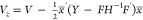. This step is completed in the time during the transition time between two batches.

Algorithm for Batch-to-Batch ILC with eMPC

• 1.Construct G_s as in eq 11 matrix using past historical data from the nominal input (U_d) and output (Y_d) profiles.
• 2.For batch 1, that is, for k = 1, apply U_k = U_s to process. This U_k and the corresponding Y_k are added to the historical data set, that is, eq 15.
• 3.Update the LTVP model of the G_k matrix with the newly added input (U_k) and output profiles (Y_k) by introducing the forgetting factor (β) as in eq 19.
• 4.Solve QPP as in eqs 23–26 for the six-state model (mass balance equations) to obtain the control input profile for the subsequent batch, that is, U_k+1.
  • (a)At each sampling time, control input is obtained by solving eq 35 and eq 36 to evaluate the off-line optimal solutions which are a piecewise affine function of the state in the form of M = Wx + V for different values of x, that is, states.
  • (b)After solving the eMPC problem for the energy equations, the first element of u(t) = M(1) is injected for next time step.
• 5.The control input profile U_k+1 will be used to update the state-space model:
  • (a)The state-space model will be updated by updating the point of linearization.
  • (b)The endpoint of target state values profile, that is, reactor temperature profile (T_r) obtained by solving the QPP in eqs 23–26 is used to evaluate the target manipulated variable (coolant flowrate) and reactor jacket temperature (T_j) using eq 48.
  • (c)This endpoint value of T_r and calculated values of T_j and coolant flowrate become the point of linearization to evaluate state-space model for every batch. This model will be updated for every batch.
• 6.This control input profile obtained (U_k+1) will be the set-point for the next MPC layer. Within batch corrections carried out are employing eMPC to deal with disturbances. This step will help us to provide the actual u_k+1 using eqs 33 and 34.
• 7.Set U_k+1 in step 2 with u_k+1, and repeat the steps till the convergence is achieved.

Results and Discussion

Batch Transesterification Model

FAME and glycerol are manufactured by transesterification (also known as alcoholysis) reaction of triglycerides (TG) present in animal fats and vegetable oils with alcohol such as methanol (M) in the presence of an alkaline or acid catalyst. Monoglycerides (MG) and diglycerides (DG) are produced as intermediates in these reactions. The three-step reaction mechanism can be shown as follows^57,58

37

38

39

The overall reaction can be given as

40

Here, k_1–8 represents the kinetic rate constants of the reactions and they are functions of reactor temperature. The batch kinetic six-state model of the three-step mechanism transesterification reaction can be stated as below

41

42

43

44

45

46

Here, k_i is the reaction rate constant which is evaluated by Arrhenius equation 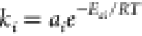. The values of pre-exponential factor (a_i) and activation energy (E_ai) for transesterification reaction at 323 K is given in Table 1:

Table 1. Values of a_i and E_ai at 323 K³².

ai in (m3 kmol–1 min–1)	a1	a2	a3	a4	a5	a6
	3.92 × 107	5.77 × 105	5.88 × 1012	0.98e10	5.35 × 103	2.15 × 104
Eai in (kJ/mol)	Ea1	Ea2	Ea3	Ea4	Ea5	Ea6
	54.99	41.55	83.08	61.25	26.86	40.11

The energy balance equations are given by

47

48

In the above equations, T_r is reactor temperature, T_j is jacket temperature, M_R is the molar mass of reactor content, V is reactor volume, ρ_R for density of reactor content, c_m,R is the molar heat capacity of reactor content, ṙ for the rate of reaction, ΔH_r for the heat of reaction, A is heat exchange surface area, U is thermal transmittance, c_w is the specific heat capacity of water, T_c (293.15 K) is the inlet jacket temperature, ṁ_c is coolant flow rate, and m_j is mass of reactor inside reactor jacket, whose values are collated in Table 2.

Table 2. Values of Parameters Used in Energy Balance Equations¹⁴.

V (m3)	1	ΔHr(kJ kmol–1)	–18,500
ρr(kg m–3)	860	AU (kJ min–1 k–1)	450
MR (kg/kmol–1)	391.4	mJ (kg)	99.69
cmR(kJ kmol–1 K–1)	1277	cw (kJ kmol–1 K–1)	4.21

The nominal reactor temperature (T_rs) profile for 15 sampling instants for a batch residence time (t_f) of 100 min was evaluated based on the FAME maximization problem. The corresponding reference FAME concentration (Y_s) can be calculated based on the 6-state plant model with an endpoint concentration of 0.8948 kmol/m³ at t_f as discussed in De et al.

Case Study Design

In this framework, batch-to-batch ILC is used to provide the reactor temperature target profile to eMPC, which will utilize energy balance equations to obtain optimal coolant flow rate in the presence of added 2% measurement noise for reactor temperature and 2% disturbance in the inlet jacket temperature. The purpose of decoupling is that the batch-to-batch ILC can take care of disturbances in the inlet jacket temperature, and eMPC can take care of disturbances in the rate of reaction of the batch transesterification process. The whole batch time (t_f) is divided into (N = 15) sampling instants.

The proposed approach was compared with a heuristic-based approach and constrained ILC approach with 2 percent measurement noise. In the heuristic approach, reactor temperature has been increased by a fixed magnitude of 2 K for subsequent batches in the six-state model until the FAME concentration reaches the desired reference trajectory.

Here, batch-to-batch correction is carried out with the help of the batch-to-batch ILC technique and correction within a batch is performed by employing eMPC, which is used to obtain an optimal coolant flowrate to achieve the desired FAME concentration, in spite of uncertainty in the process. As the MPC problem is computationally challenging, to curb that, the eMPC method is utilized, where the optimization problem is solved in a manner that optimal solutions are obtained as an explicit function of parameters and reference vectors a priori, which can be obtained offline.⁵¹

Case Study 1: Uncertainty in E_a3

In this case study, we have introduced a disturbance of 2% increase in the E_a3 (activation energy) in the batch transesterification model while injecting the nominal reactor temperature profile (T_rs), due to which there is a drop in the FAME concentration from 0.8948 to 0.8492 kmol/m³ at t_f due to plant-model mismatch. To overcome this problem, we employ the combination of batch-to-batch ILC and eMPC. The data thus obtained are saved in a historical database, which is used to construct the LTVP model, G_k.

The lower and upper bound for reactor temperature change (ΔU_k+1) between two consecutive batches were kept as 0 to 15 K, respectively. The QPP was solved using quadprog in MATLAB to obtain the reactor temperature profile.⁴⁴ Parameters selected to carry out the batch-to-batch ILC can be listed as Q = diag(0.5I_5×5, 0.7I_6×6, 2I_4×4), R = (10e – 7)I and β = 0.9.

The reactor temperature obtained after solving QPP is given as the set-point for the next layer, (eMPC). In this step, we solve the constrained MPC objective problem as a mpQP with the help of the MPT3 toolbox in MATLAB to obtain the optimized reactor temperature profile. Here, we have also introduced noise in the reactor temperature measurement. After implementation of eMPC, six critical regions were formed when sampling time was 30 s. Moreover, computational time has been reduced from 7 s for MPC to 2.6 s for eMPC, as seen from Table 6.

Table 6. MPC and eMPC: Computational Savings.

computational time of MPC	7 s
computational time of eMPC	2.6 s

Table 4. RMSE Comparison Study.

RMSE
	case study 1			case study 2
batch number	heuristic-based approach	batch-to-batch ILC	proposed approach	heuristic-based approach	batch-to-batch ILC	proposed approach
batch 1	0.0506	0.056	0.0506	0.0639	0.0639	0.0639
batch 2	0.0409	0.0313	0.0494	0.0547	0.0582	0.0625
batch 3	0.0338	0.0309	0.0393	0.0474	0.0311	0.0515
batch 4	0.0297	0.0414	0.0302	0.0425	0.0264	0.0432
batch 5	0.0289	0.0531		0.0398	0.0409	0.0364
batch 6	0.0309	0.0633		0.0392	0.0575	0.033
batch 7	0.0346			0.0402	0.0551
batch 8	0.0391			0.0424	0.0683
batch 9	0.0438			0.0453	0.0594
batch 10	0.0486			0.0485
batch 11	0.0531			0.0518
batch 12	0.0574			0.0551
batch 13				0.0583
batch 14				0.0613
batch 15				0.0641
batch 16				0.0666
batch 17				0.069
batch 18				0.0712
batch 19				0.0732
batch 20				0.075

By the proposed approach, FAME endpoint concentration has been improved from 0.8492 kmol/m³ for batch 1 to 0.884 kmol/m³ for batch 4 (see Figure 2). The reactor temperature tracking obtained by solving mpQP is shown in Figure 4. It is observed from Figure 4 that with each batch, tracking the performance of reactor temperature has been improved. Coolant flow rate that achieves the reference temperature profile is shown in Figure 5. These optimized reactor temperature profiles result in the FAME concentration profile, as shown in Figure 3, obtained by simulating the batch transesterification plant represented by eqs 41–46. The value of endpoint error, the difference between reference and optimized endpoint FAME concentration, has been dropped from 0.0456 for batch 1 to 0.0136 for batch 4, which can be shown in Tables 3–5. Similarly, RMSE values have been reduced from 0.0506 for batch 1 to 0.0302 for batch 4. The values for endpoint tracking error of FAME concentration, RMSE, and endpoint concentration for different batches have been tabulated in Tables 3–5. Further, the adoption of eMPC makes the computation of the solution significantly faster compared to normal MPC, as indicated in Table 6.

Figure 2.

Optimized FAME concentration profile for different batches (case study 1).

Figure 4.

Reactor temperature tracking profiles using eMPC for different batches (case study 1).

Figure 5.

Coolant flowrate profiles for different batches (case study 1).

Figure 3.

Optimized reactor temperature profiles for different batches (case study 1).

Table 3. End Point Tracking Error Comparison Study.

end point tracking error
	case study 1			case study 2
batch number	heuristic-based approach	batch-to-batch ILC	proposed approach	heuristic-based approach	batch-to-batch ILC	proposed approach
batch 1	0.0456	0.0456	0.0456	0.0602	0.0602	0.0602
batch 2	0.0422	0.0374	0.0375	0.0570	0.0477	0.0526
batch 3	0.0409	0.0299	0.0262	0.0540	0.0356	0.0408
batch 4	0.0358	0.0228	0.0136	0.0510	0.0353	0.0301
batch 5	0.03288	0.0163		0.0482	0.0334	0.02
batch 6	0.0299	0.0101		0.0454	0.029	0.0146
batch 7	0.027			0.0427	0.0233
batch 8	0.0242			0.0401	0.0233
batch 9	0.0215			0.0375	0.0134
batch 10	0.0189			0.0350
batch 11	0.0163			0.0326
batch 12	0.0138			0.0302
batch 13				0.0279
batch 14				0.0257
batch 15				0.0235
batch 16				0.0214
batch 17				0.0193
batch 18				0.0173
batch 19				0.0154
batch 20				0.0135

Table 5. End Point FAME Concentration Comparison Study.

end point FAME concentration (kmol/m3)
	case study 1			case study 2
batch number	heuristic-based approach	batch-to-batch ILC	proposed approach	heuristic-based approach	batch-to-batch ILC	proposed approach
batch 1	0.8492	0.8492	0.8492	0.8346	0.8346	0.8346
batch 2	0.8526	0.8574	0.8573	0.8378	0.8471	0.8422
batch 3	0.8539	0.8649	0.8686	0.8408	0.8592	0.8540
batch 4	0.859	0.8720	0.8812	0.8438	0.8595	0.8647
batch 5	0.862	0.8785		0.8466	0.8614	0.8748
batch 6	0.865	0.8847		0.8494	0.8658	0.8802
batch 7	0.8678			0.8521	0.8715
batch 8	0.8706			0.8547	0.8715
batch 9	0.8733			0.8573	0.8814
batch 10	0.8759			0.8598
batch 11	0.8785			0.8622
batch 12	0.881			0.8646
batch 13				0.8646
batch 14				0.8691
batch 15				0.8713
batch 16				0.8734
batch 17				0.8755
batch 18				0.8775
batch 19				0.8794
batch 20				0.8813

A comparative study has been performed between heuristic, constrained batch-to-batch ILC and the abovementioned approach (combination of batch-to-batch ILC and eMPC). The heuristic-based approach is the best method available to plant engineers to handle plant-model mismatch under uncertainties. It is observed that while the heuristic-based approach took 12 batches, only 6 batches were needed for constrained batch-to-batch ILC only for convergence. However, both responses were slower than the proposed ILC-eMPC, which took 4 batches for convergence (see Tables 3–5). This shows that the proposed arrangement is much better than heuristic-based approach and constrained batch-to-batch ILC approach as the former achieved convergence at a lower number of batches. It is also observed that root-mean-square error (RMSE) of e_k showed faster tracking performance of proposed arrangement as compared to the heuristic-based approach.

Case Study 2: Uncertainty in TG Inlet Concentration

The proposed approach has also been applied to the same plant model with an introduction of a 3 percent decrease in the TG inlet concentration and a 2 percent increase in E_a3. For carrying out batch-to-batch ILC, it was assumed that disturbance in TG inlet concentration and increase in E_a3 occurred in 32nd batch as a fixed parametric uncertainty and it remains fixed for further batch operations. FAME end-point concentration was reduced from 0.8948 to 0.8346 kmol/m³ due to plant-model mismatch. Following the same algorithm, it was observed that we were able to achieve the desired convergence at 6th batch as shown in Figure 6. This proposed approach was compared with the heuristic-based approach and constrained batch-to-batch ILC approach. It was observed that convergence was achieved at 20th batch for the heuristic-based approach and 9th batch for the constrained batch-to-batch ILC approach, as shown in Tables 3–5. Coolant flowrate for this case study is shown in Figure 8. Optimized FAME concentration and corresponding optimized reactor temperature profile are shown in Figures 6 and 7, respectively. The tracking performance of reactor temperature is shown in Figure 9. Moreover, RMSE tracking performance was much better for the proposed approach as compared to the heuristic-based approach and constrained batch-to-batch ILC approach.

Figure 6.

Optimized FAME concentration profile for different batches (case study 2).

Figure 8.

Coolant flowrate for different batches (case study 2).

Figure 7.

Optimized reactor temperature profiles for different batches (case study 2).

Figure 9.

Reactor temperature tracking profiles using eMPC for different batches (case study 2).

Conclusions

In this work, we have used a combination of batch-to-batch ILC and eMPC for optimizing FAME concentration in batch transesterification. A six-state model of batch transesterification, with two case studies, disturbance in E_a3 (case study 1) and disturbance in both E_a3 and TG inlet concentration (case study 2) has been used for batch-to-batch ILC to obtain the reactor temperature set-point trajectory for the next layer, eMPC. It is observed that with the progress of each batch, tracking performance is improved, which provides an added advantage of this arrangement. Moreover, eMPC also reduces the computational time as compared to MPC. The main purpose of this decoupling is that fluctuations in the rate of reaction are taken care of by the eMPC part and disturbance in heat transfer coefficient is taken care by batch-to-batch ILC, complementing each other. The proposed approach results were also compared with the heuristic-based approach and constrained batch-to-batch ILC approach. The proposed approach was much superior and cost-efficient than the heuristic-based approach and constrained batch-to-batch ILC approach.

The authors declare no competing financial interest.

References

- Gupta S. S.; Shastri Y.; Bhartiya S.. Optimization of the Integrated Downstream Processing of Microalgae for Biomolecule Production. Sustainable Downstream Processing of Microalgae for Industrial Application; CRC Press, 2019; pp 317–350. [Google Scholar]
- Yusoff M. F. M.; Xu X.; Guo Z. Comparison of fatty acid methyl and ethyl esters as biodiesel base stock: a review on processing and production requirements. J. Am. Oil Chem. Soc. 2014, 91, 525–531. 10.1007/s11746-014-2443-0. [DOI] [Google Scholar]
- De R.; Bhartiya S.; Shastri Y. Multi-objective optimization of integrated biodiesel production and separation system. Fuel 2019, 243, 519–532. 10.1016/j.fuel.2019.01.132. [DOI] [Google Scholar]
- De R.; Bhartiya S.; Shastri Y. Parameter estimation and optimal control of a batch transesterification reactor: An experimental study. Chem. Eng. Res. Des. 2020, 157, 1–12. 10.1016/j.cherd.2020.02.027. [DOI] [Google Scholar]
- Krishnan A.; Kosanovich K. A. Batch reactor control using a multiple model-based controller design. Can. J. Chem. Eng. 1998, 76, 806–815. 10.1002/cjce.5450760417. [DOI] [Google Scholar]
- Mhaskar P.; Garg A.; Corbett B.. Batch Process Modeling and Control: Background. Modeling and Control of Batch Processes; Springer, 2019; pp 11–19. [Google Scholar]
- Wang D. Robust data-driven modeling approach for real-time final product quality prediction in batch process operation. IEEE Trans. Industr. Inform. 2011, 7, 371–377. 10.1109/tii.2010.2103401. [DOI] [Google Scholar]
- Corbett B.; Mhaskar P. Data-driven modeling and quality control of variable duration batch processes with discrete inputs. Ind. Eng. Chem. Res. 2017, 56, 6962–6980. 10.1021/acs.iecr.6b03137. [DOI] [Google Scholar]
- Ao T.; Dong X.; Zhizhong M. Batch-to-batch iterative learning control of a batch polymerization process based on online sequential extreme learning machine. Ind. Eng. Chem. Res. 2009, 48, 11108–11114. 10.1021/ie9007979. [DOI] [Google Scholar]
- Lee K. S.; Chin I.-S.; Lee H. J.; Lee J. H. Model predictive control technique combined with iterative learning for batch processes. AIChE J. 1999, 45, 2175–2187. 10.1002/aic.690451016. [DOI] [Google Scholar]
- Lee K. S.; Lee J. H. Iterative learning control-based batch process control technique for integrated control of end product properties and transient profiles of process variables. J. Process Control 2003, 13, 607–621. 10.1016/s0959-1524(02)00096-3. [DOI] [Google Scholar]
- Aziz N.; Mujtaba I. Optimal operation policies in batch reactors. Chem. Eng. J. 2002, 85, 313–325. 10.1016/s1385-8947(01)00169-3. [DOI] [Google Scholar]
- Joshi T.; Goyal V.; Kodamana H. A Novel Dynamic Just-in-Time Learning Framework for Modeling of Batch Processes. Ind. Eng. Chem. Res. 2020, 59, 19334–19344. 10.1021/acs.iecr.0c02979. [DOI] [Google Scholar]
- Kern R.; Shastri Y. Advanced control with parameter estimation of batch transesterification reactor. J. Process Control 2015, 33, 127–139. 10.1016/j.jprocont.2015.06.006. [DOI] [Google Scholar]
- Mhaskar P.; Garg A.; Corbett B.. Modeling and Control of Batch Processes: Theory and Applications; Springer, 2018. [Google Scholar]
- Kim S.; Kano M.; Hasebe S.; Takinami A.; Seki T. Long-term industrial applications of inferential control based on just-in-time soft-sensors: Economical impact and challenges. Ind. Eng. Chem. Res. 2013, 52, 12346–12356. 10.1021/ie303488m. [DOI] [Google Scholar]
- Patwardhan S. C.; Narasimhan S.; Jagadeesan P.; Gopaluni B.; L. Shah S. L. Nonlinear Bayesian state estimation: A review of recent developments. Control Eng. Pract. 2012, 20, 933–953. 10.1016/j.conengprac.2012.04.003. [DOI] [Google Scholar]
- Ghahremani E.; Kamwa I. Online state estimation of a synchronous generator using unscented Kalman filter from phasor measurements units. IEEE Trans. Energy Convers. 2011, 26, 1099–1108. 10.1109/tec.2011.2168225. [DOI] [Google Scholar]
- Terwiesch P.; Agarwal M.; Rippin D. W. Batch unit optimization with imperfect modelling: a survey. J. Process Control 1994, 4, 238–258. 10.1016/0959-1524(94)80045-6. [DOI] [Google Scholar]
- Bonvin D. Optimal operation of batch reactors—a personal view. J. Process Control 1998, 8, 355–368. 10.1016/s0959-1524(98)00010-9. [DOI] [Google Scholar]
- Clarke-Pringle T. L.; MacGregor J. F. Optimization of molecular-weight distribution using batch-to-batch adjustments. Ind. Eng. Chem. Res. 1998, 37, 3660–3669. 10.1021/ie980058a. [DOI] [Google Scholar]
- Ahn H.-S.; Chen Y.; Moore K. L. Iterative learning control: Brief survey and categorization. IEEE Trans. Syst. Man Cybern. 2007, 37, 1099–1121. 10.1109/tsmcc.2007.905759. [DOI] [Google Scholar]
- Liu J. Fuzzy modularity and fuzzy community structure in networks. Eur. Phys. J. B 2010, 77, 547–557. 10.1140/epjb/e2010-00290-3. [DOI] [Google Scholar]
- Zhang Y.; Fan Y.; Zhang P. Combining kernel partial least-squares modeling and iterative learning control for the batch-to-batch optimization of constrained nonlinear processes. Ind. Eng. Chem. Res. 2010, 49, 7470–7477. 10.1021/ie1004702. [DOI] [Google Scholar]
- Sanzida N.; Nagy Z. K. Iterative learning control for the systematic design of supersaturation controlled batch cooling crystallisation processes. Comput. Chem. Eng. 2013, 59, 111–121. 10.1016/j.compchemeng.2013.05.027. [DOI] [Google Scholar]
- Flores-Cerrillo J.; MacGregor J. F. Iterative learning control for final batch product quality using partial least squares models. Ind. Eng. Chem. Res. 2005, 44, 9146–9155. 10.1021/ie048811p. [DOI] [Google Scholar]
- Cueli J.; Bordons C.. Iterative nonlinear control of a semibatch reactor. Stability analysis. Proceedings of the 44th IEEE Conference on Decision and Control; IEEE, 2005; pp 2071–2076.
- Bemporad A.; Morari M.; Dua V.; Pistikopoulos E. N. The explicit linear quadratic regulator for constrained systems. Automatica 2002, 38, 3–20. 10.1016/s0005-1098(01)00174-1. [DOI] [Google Scholar]
- Marquez-Ruiz A.; Loonen M.; Saltık M. B.; Özkan L. Model Learning Predictive Control for Batch Processes: A Reactive Batch Distillation Column Case Study. Ind. Eng. Chem. Res. 2019, 58, 13737–13749. 10.1021/acs.iecr.8b06474. [DOI] [Google Scholar]
- Lee J. H.; Lee K. S. Iterative learning control applied to batch processes: An overview. Control Eng. Pract. 2007, 15, 1306–1318. 10.1016/j.conengprac.2006.11.013. [DOI] [Google Scholar]
- Gupta A.; Pravin P.; Bhartiya S.; Gudi R. D. Iterative learning estimation with lean measurements. IFAC-PapersOnLine 2016, 49, 71–76. 10.1016/j.ifacol.2016.03.031. [DOI] [Google Scholar]
- De R.; Bhartiya S.; Shastri Y. Constrained iterative learning control of batch transesterification process under uncertainty. Control Eng. Pract. 2020, 103, 104580. 10.1016/j.conengprac.2020.104580. [DOI] [Google Scholar]
- De Souza G.; Odloak D.; Zanin A. C. Real time optimization (RTO) with model predictive control (MPC). Comput. Chem. Eng. 2010, 34, 1999–2006. 10.1016/j.compchemeng.2010.07.001. [DOI] [Google Scholar]
- Xue S.; Zhao Z.; Liu F. Latent variable point-to-point iterative learning model predictive control via reference trajectory updating. Eur. J. Control 2022, 65, 100631. 10.1016/j.ejcon.2022.100631. [DOI] [Google Scholar]
- Zhou C.; Jia L.; Zhou Y. Tube-based iterative-learning-model predictive control for batch processes using pre-clustered just-in-time learning methodology. Chem. Eng. Sci. 2022, 259, 117802. 10.1016/j.ces.2022.117802. [DOI] [Google Scholar]
- Zhang W.; Ma J.; Wang L.; Jiang F. Particle-swarm-optimization-based 2D output feedback robust constraint model predictive control for batch processes. IEEE Access 2022, 10, 8409–8423. 10.1109/access.2022.3143691. [DOI] [Google Scholar]
- Saltik B.; Jayawardhana B.; Cherukuri A.. Koopman Operator based Iterative Learning and Model Predictive Control for Repetitive Nonlinear Systems. 61st IEEE Conference on Decision and Control; IEEE, 2022.
- Zhang K.; Xu F.; Xu X. Robust iterative learning model predictive control for repetitive motion of maglev planar motor. IET Electr. Power Appl. 2022, 16, 1189. 10.1049/elp2.12213. [DOI] [Google Scholar]
- Zuliani R.; Balta E. C.; Rupenyan A.; Lygeros J.. Batch model predictive control for selective laser melting. 2022 European Control Conference (ECC); IEEE, 2022; pp 1560–1565.
- Oh S.-K.; Lee J. M. Iterative learning model predictive control for constrained multivariable control of batch processes. Comput. Chem. Eng. 2016, 93, 284–292. 10.1016/j.compchemeng.2016.07.011. [DOI] [Google Scholar]
- Laurí D.; Lennox B.; Camacho J. Model predictive control for batch processes: Ensuring validity of predictions. J. Process Control 2014, 24, 239–249. 10.1016/j.jprocont.2013.11.005. [DOI] [Google Scholar]
- Jia L.; Han C.; Chiu M.-s. Dynamic R-parameter based integrated model predictive iterative learning control for batch processes. J. Process Control 2017, 49, 26–35. 10.1016/j.jprocont.2016.11.003. [DOI] [Google Scholar]
- Penlidis A.; Ponnuswamy S.; Kiparissides C.; O’Driscoll K. Polymer reaction engineering: modelling considerations for control studies. Chem. Eng. J. 1992, 50, 95–107. 10.1016/0300-9467(92)80013-z. [DOI] [Google Scholar]
- Xiong Z.; Zhang J. Product quality trajectory tracking in batch processes using iterative learning control based on time-varying perturbation models. Ind. Eng. Chem. Res. 2003, 42, 6802–6814. 10.1021/ie034006j. [DOI] [Google Scholar]
- Afram A.; Janabi-Sharifi F. Theory and applications of HVAC control systems–A review of model predictive control (MPC). Build. Environ. 2014, 72, 343–355. 10.1016/j.buildenv.2013.11.016. [DOI] [Google Scholar]
- Mate S.; Bhartiya S.; Nataraj P. Multiparametric Nonlinear MPC: A region free approach. IFAC-PapersOnLine 2020, 53, 11374–11379. 10.1016/j.ifacol.2020.12.548. [DOI] [Google Scholar]
- Hariprasad K.; Bhartiya S. A computationally efficient robust tube based MPC for linear switched systems. Nonlinear Anal.: Hybrid Syst. 2016, 19, 60–76. 10.1016/j.nahs.2015.07.002. [DOI] [Google Scholar]
- Hariprasad K.; Bhartiya S.. Adaptive robust model predictive control of nonlinear systems using tubes based on interval inclusions. 53rd IEEE Conference on Decision and Control; IEEE, 2014; pp 2032–2037.
- Atmaram L. L.; Kodamana H. Successive Linearization based Stochastic Model Predictive Control for batch processes described by DAEs. IFAC-PapersOnLine 2020, 53, 380–385. 10.1016/j.ifacol.2020.06.064. [DOI] [Google Scholar]
- Gupta A.; Bhartiya S.; Nataraj P. A novel approach to multiparametric quadratic programming. Automatica 2011, 47, 2112–2117. 10.1016/j.automatica.2011.06.019. [DOI] [Google Scholar]
- Mesbah A. Stochastic model predictive control: An overview and perspectives for future research. IEEE Control Syst. Mag. 2016, 36, 30–44. 10.1109/MCS.2016.2602087. [DOI] [Google Scholar]
- Feller C.; Johansen T. A.; Olaru S. An improved algorithm for combinatorial multi-parametric quadratic programming. Automatica 2013, 49, 1370–1376. 10.1016/j.automatica.2013.02.022. [DOI] [Google Scholar]
- Bemporad A.; Filippi C.. Suboptimal explicit MPC via approximate multiparametric quadratic programming. Proceedings of the 40th IEEE Conference on Decision and Control; IEEE, 2001; pp 4851–4856. (Cat. No. 01CH37228).
- Tøndel P.; Johansen T. A.; Bemporad A. An algorithm for multi-parametric quadratic programming and explicit MPC solutions. Automatica 2003, 39, 489–497. 10.1016/S0005-1098(02)00250-9. [DOI] [Google Scholar]
- Bakaráč P.; Holaza J.; Kalúz M.; Klaučo M.; Löfberg J.; Kvasnica M.. Explicit MPC based on approximate dynamic programming. 2018 European Control Conference (ECC); IEEE, 2018; pp 1172–1177.
- Mönnigmann M.; Jost M.. Vertex based calculation of explicit MPC laws. 2012 American Control Conference (ACC); IEEE, 2012; pp 423–428.
- Noureddini H.; Zhu D. Kinetics of transesterification of soybean oil. J. Am. Oil Chem. Soc. 1997, 74, 1457–1463. 10.1007/s11746-997-0254-2. [DOI] [Google Scholar]
- Chanpirak A.; Weerachaipichasgul W.. Improvement of biodiesel production in batch transesterification process. Proceedings of the International MultiConference of Engineers and Computer Scientists, II; International Association of Engineers, 2017.