Threshold condition and non pharmaceutical interventions’s control strategies for elimination of COVID-19

Abstract

In this work we focus on the eradication of the COVID-19 infection with the help of almost Non Pharmaceutical Interventions(NPIs), using mathematical modelling. First the basic reproduction number $R_0$ is investigated. Then, on the basis of sensitivity test of $R_0$, the most active/sensitive parameters are presented in detail. Non Pharmaceutical Interventions(NPIs) are applied to control the sensitive parameters. The major NPIs are, stay home (isolation), sanitizers (wash hands), Treatment of side effects of infection, like throat infection etc and face mask. These NPIs helps in mitigation and reducing the size of outbreak of the disease. Threshold condition for global stability of the disease free state is investigated.The NPI’s are used in different ratios to formulate a strategy. The results of these strategies are validated using Matlab software.

Introduction

COVID-19 is a highly infectious disease, which is caused by a virus called Severe Acute Respiratory Syndrome coronavirus 2, or SARS-CoV-2. The virus transmission among human population, from person to person is very rapid specially those in close contact (within about 6 feet, or 2 meters). The virus spreads by respiratory droplets released when an infected individual coughs, sneezes or talks. These droplets can be inhaled or directly reach the mouth or nose of a nearby person with medium of air. A person can catch infection from contaminated surfaces, however this isn’t considered to be a main way it spreads through [1].

Coronaviruses infact represents a big family. This family causes different types of infections. The infection ranges from common cold/flue to the most severe infection like severe acute respiratory syndrome and MERS; middle east respiratory syndrome [2]. The novel COVID-19 first emerged in December, 2019, Wuhan, China, in the form of severe cases of pneumonia and respiratory problems. The correct etiology of the infection could not be traced that time. WHO reported the virus as a novel coronavirus (2019-nCoV). The disease was named as severe acute respiratory syndrome coronavirus-2 (SARS-CoV-2). The virus was first identified from a single individual. Subsequently the virus was verified in sixteen more cases [3], [4].

It is expected that the virus might be bat origin [5], and the infection transmission might be initiated from a seafood market (Huanan Seafood Wholesale Market) of China [6], [9]. Currently 7,597,304 cases of the disease as been confirmed and 423,844 deaths has occurred as of June 12, 2020, world wide [10].

About $75\%$ of the victims of COVID-19 don’t develop symptoms of the disease and recovered naturally [29]. $20\%$ of the exposed individuals develop symptoms. The most common symptoms of COVID-19 are tiredness, fever and dry cough. Some patients may have aches and pains, runny nose, nasal congestion, Muscle aches, Chills, Loss of taste or smell or both, Headache, Chest pain and sore throat. Other less common symptoms have been reported, such as rash, nausea, vomiting and diarrhea. These symptoms are usually mild and starts slowly and gradually. Most symptomatic individuals (about 80%) recover from the disease without needing special treatment. In children and young adults, COVID-19 is generally minor. However, for some people it can cause serious illness. This type of severe attack of the virus may cause death. In some cases the attack may result SARS (severe acute respiratory syndrome) or pneumonia. The symptoms of infection appears in 2–14 days [7], [15]. The recovery time of mild cases is approximately 2 weeks and in severe/critical cases the recovery may take 3–6 weeks [16]. The individuals who developed severe form of disease, the medium time to dyspnea ranges from 5–8 days. The average time to acute respiratory distress syndrome (ARDS) varies from 8 days to 12 days. The averae time to intensive care at vent bol (ventilated class) ranges from 10–12 days [18], [17], [19], [20].The recovered individuals of disease can have antibodies for at least two weeks, long-term data are still lacking [21].

The coronavirus (2019-nCoV) is genetically related to the coronavirus that caused the SARS-2003, however the diseases they caused are quite different [8]. The genetic features and some clinical findings of the infection have been reported recently [9], [22], [23]. International air travel contributed the international spread of the infection. The infection has got global attention regarding its elimination and control [24].

The whole world is highly concerned with drastic future forecast of the disease. The scientists and researchers, therefore focus the development of mathematical model. The model not only helps estimating dynamics of the transmission of the virus but other important forecasts. Recent mathematical modeling includes [6], [25], [26], [27]. These models mainly focused the transmission/spreading of coronavirus or basic reproduction number of coronavirus, $\left(R_0\right)$. The authors followed intrinsic growth rate and the serial intervals. Wu et al. in their study focus the forecasting and Newscasting of the novel coronavirus both nationally and internationally. The authors used Markov Chain Monte Carlo methods in their study [25].

Some novel corona models discuss the origin (bat), the route of transmission/spreading (seafood market) and reservoir class [14], [28]. Atangana in his recent work focus the importance of lockdown and Vaccination [11]. For more study on COVID-19 the reader is reffered to [12], [13], [30], [31].

We, in this study focus three dynamics of the disease:

• •The formulation of mathematical model.
• •To investigate the ratio of different interventions to formulate a control strategy.
• •To find a rule to stop re-attack of the disease to the community

From the proposed model we find the initial transmission rate of the disease. With help of sensitivity test, we select the parameters playing most important role in transmission of the disease. The sign of the sensitivity indexes help in deciding an increase or decrease in the concerned parameters. We combine different interventions in particular ratio and formulate a strategy. The effect of different strategies on disease control is shown graphically to facilitate strategy selection for the agencies fighting against COVID-19.

The re-attack of COVID-19 is really heartbroken issue of the scientists. To address the issue we find a threshold condition. If the magnitude of interventions is capable of disease elimination and satisfy the threshold condition. Then there is guarantee for global stability of the disease free state in the community.

Model formulation

The population concerned with the disease is divided into the following six compartments:

• •S; The susceptible human class.
• •E; The Exposed/latency class.
• •$I_1$; The infectious class with disease symptoms.
• •$I_v$; The vent Bol class, critically infected individuals kept on ventilator.
• •$I_2$; The Asymptomatic infectious class.
• •R; The Recovered class.
• •W; The class of contaminated stuff or surfaces.

The susceptible human after catching infection from the infectious humans (both symptomatic and asymptomatic) or contaminated surfaces/stuff moves to the exposed class (E). The $20\%$ of the exposed individuals move to symptomatic infectious class $\left(I_1\right)$ and the rest are placed in asymptomatic infectious class $\left(I_2\right)$, after completing the transition period ${\eta }_1$ at E. About $5\%$ percent of the infectious (both symptomatic and asymptomatic) individuals face severe form of infection and are put on ventilator and are placed in $\left(I_v\right)$. $49\%$ of the vent bols dies due to disease. The symptomatic infectious individuals are isolated. Some of the infectious individuals dies due to disease and the rest moves to the recovered class R. The recovered individuals loose immunity at the rate ${\beta }_3$ and rejoin the susceptible class. N denotes the density of human population.

The Mathematical model of the disease is given by the following set of coupled differential equation:

$$\left\{\begin{array}{c}\dot{S}={\mathrm{\Gamma }}_h+{\beta }_{3}R-(\frac{{\beta }_1(I_1+\gamma I_2)}{N}S+{\beta }_2\mathit{WS})-\mu S\hfill \\ \dot{E}=(\frac{{\beta }_1(I_1+\gamma I_2)}{N}S+{\beta }_2\mathit{WS})-{\eta }_{1}E-\mu E\hfill \\ \dot{I_1}=(1-\delta ){\eta }_{1}E-(K+\mu )I_1\hfill \\ \dot{I_v}=K\beta I_1+K{\alpha }_2{I}_2-({\alpha }_1+D_2+\mu )I_v\hfill \\ \dot{I_2}=\delta {\eta }_{1}E-(K+\mu )I_2\hfill \\ \dot{R}=(1-\beta ){\mathit{KI}}_1+{\alpha }_1{I}_v+(1-{\alpha }_2){\mathit{KI}}_2-\mu R-{\beta }_{3}R\hfill \\ \dot{W}={\theta }_1{I}_1+{\theta }_2{I}_2-\epsilon W\text{.}\hfill \end{array}\right)$$ (1)

The following table (1) contains the values of the different parameters used in the model (1). Table 2 .

Table 1.

Table of the Values of parameters.

Notation	Parameter definition	Value	Source
${\mathrm{\Gamma }}_h$	Humans recruitment rate	$0.0015875\times N{\mathit{day}}^{-1}$	[33]
$\mu$	Humans natural mortality rate	$0.00004{\mathit{day}}^{-1}$	[33], [35]
$1/\epsilon$	$\epsilon$ is the life time of virus on W	$0.1{\mathit{day}}^{-1}$	[28]
$1/{\eta }_1$	${\eta }_1$ is the incubation period of human	$0.1923{\mathit{day}}^{-1}$	[44], [28]
K	The transition period at $I_1$	$2-6\mathit{weaks}$	[32]
${\alpha }_1$	The ratio of recovery of critical class	$51\%$	[37]
${\alpha }_2$	The of ratio asymptomatic moving to vent bol	$2\%$	[39], [40]
$\delta$	The of ratio exposed moving to asymptomatic	$75\%$	[29]
${\beta }_1$	The transmission rate of infection from $I_1$ to S	$0.65{\mathit{day}}^{-1}$	[28]
${\beta }_2$	The transmission rate of infection from stuff	$0.165{\mathit{day}}^{-1}$	[28]
${\theta }_1$	The shedding coeffieient of $I_1$ on W	0.5	[28]
${\theta }_2$	The shedding coeffieient of $I_2$ on W	0.5	[28]
$\gamma$	The multiple of the transmissibility	$0.5$	[28]
	of $I_2$ to that of $I_1$
$D_2$	Disease induced death ratio of vent bol	$49\%$	[38]
$\beta$	The ratio of symptomatic moving to vent bol	$5\%$	[36]
${\beta }_3$	The Immunity loosing rate of recovered indivivduals	$0.066{\mathit{day}}^{-1}$	[21]

Table 2.

Sensitivity indices of parameters.

Parameter	value	index	Parameter	value	index
$\delta$	$0.75$	$-0.0074$	$\mu$	$0.00004$	$-0.9963$
${\beta }_1$	$0.65$	$0.123$	${\eta }_1$	$0.1923$	$0.00020797$
${\beta }_2$	$0.165$	$0.9877$	${\mathrm{\Gamma }}_h$	$0.0015875$	$0.9877$
${\theta }_1$	$0.5$	$0.2469$	${\theta }_2$	$0.5$	$0.7408$
K	$0.041429$	$-0.999$	$\gamma$	0.5	$0.0074$
$\epsilon$	$0.1$	$-0.9877$

Model analysis

Here, in this Section 3 properties of the model; Disease-Free-Equilibrium, Invariant region and the Basic Reproduction Number would be discussed.

Invariant region

The state variables and parameters used in the model are all non-negative because the model is concerned with the living population.

$$\dot{N}={\mathrm{\Gamma }}_h-\mu N-D_2{I}_v,$$ (2)

From Eq. (2) we have

$$\dot{N}⩽{\mathrm{\Gamma }}_h-\mu N\text{.}$$

Solving this equation, we have

$$N⩽N\left(0\right)e^{-\mu .t}+\frac{{\mathrm{\Gamma }}_h}{\mu }\left(1-e^{-\mu .t}\right)\Rightarrow N⩽\frac{{\mathrm{\Gamma }}_h}{\mu }\mathit{whent}\to \infty$$

So we claim the following proposition:

Proposition 0.1

[34] The region $\mathrm{\Omega }$, given by:

$\mathrm{\Omega }=\left[(S,E,I_1,I_v,I_2,R,W)\in R_{+}^7,N⩽\frac{{\mathrm{\Gamma }}_h}{\mu }\right]$. is positively invariant domain, and the model is epidemiologically and mathematically well posed and all the trajectories are forward bounded.

Disease reproduction number

The number of secondary infections caused by a single primary infection in completely susceptible population is called $R_0$ or the disease reproduction rate. The Reproduction number is find by next generation matrix [35], [33].

$R_0=\rho (-{\mathit{FV}}^{-1}),$where $\rho$ is spectral radius.

$$f=\left(\begin{array}{c}\hfill f_1\hfill \\ \hfill f_2\hfill \\ \hfill f_3\hfill \\ \hfill f_4\hfill \\ \hfill f_5\hfill \end{array}\right)=\left(\begin{array}{c}\hfill (\frac{{\beta }_1(I_1+\gamma I_2)}{N}S+{\beta }_2\mathit{WS})\hfill \\ \hfill 0\hfill \\ \hfill 0\hfill \\ \hfill 0\hfill \\ \hfill 0\hfill \end{array}\right)$$

The column in matrix f denotes the individuals who get infected.

$F=\left(\begin{array}{ccccc}\hfill \frac{\partial \left(f_1\right)}{\partial \left(E\right)}\hfill & \hfill \frac{\partial \left(f_1\right)}{\partial \left(I_1\right)}\hfill & \hfill \frac{\partial \left(f_1\right)}{\partial \left(I_v\right)}\hfill & \hfill \frac{\partial \left(f_1\right)}{\partial \left(I_2\right)}\hfill & \hfill \frac{\partial \left(f_1\right)}{\partial \left(W\right)}\hfill \\ \hfill \frac{\partial \left(f_2\right)}{\partial \left(E\right)}\hfill & \hfill \frac{\partial \left(f_2\right)}{\partial \left(I_1\right)}\hfill & \hfill \frac{\partial \left(f_2\right)}{\partial \left(I_v\right)}\hfill & \hfill \frac{\partial \left(f_2\right)}{\partial \left(I_2\right)}\hfill & \hfill \frac{\partial \left(f_2\right)}{\partial \left(W\right)}\hfill \\ \hfill \frac{\partial \left(f_3\right)}{\partial \left(E\right)}\hfill & \hfill \frac{\partial \left(f_3\right)}{\partial \left(I_1\right)}\hfill & \hfill \frac{\partial \left(f_3\right)}{\partial \left(I_v\right)}\hfill & \hfill \frac{\partial \left(f_3\right)}{\partial \left(I_2\right)}\hfill & \hfill \frac{\partial \left(f_3\right)}{\partial \left(W\right)}\hfill \\ \hfill \frac{\partial \left(f_4\right)}{\partial \left(E\right)}\hfill & \hfill \frac{\partial \left(f_4\right)}{\partial \left(I_1\right)}\hfill & \hfill \frac{\partial \left(f_4\right)}{\partial \left(I_v\right)}\hfill & \hfill \frac{\partial \left(f_4\right)}{\partial \left(I_2\right)}\hfill & \hfill \frac{\partial \left(f_4\right)}{\partial \left(W\right)}\hfill \\ \hfill \frac{\partial \left(f_5\right)}{\partial \left(E\right)}\hfill & \hfill \frac{\partial \left(f_5\right)}{\partial \left(I_1\right)}\hfill & \hfill \frac{\partial \left(f_5\right)}{\partial \left(I_v\right)}\hfill & \hfill \frac{\partial \left(f_5\right)}{\partial \left(I_2\right)}\hfill & \hfill \frac{\partial \left(f_5\right)}{\partial \left(W\right)}\hfill \end{array}\right)$$=\left(\begin{array}{ccccc}\hfill 0\hfill & \hfill \frac{{\beta }_{1}S}{N}\hfill & \hfill 0\hfill & \hfill \frac{\gamma {\beta }_{1}S}{N}\hfill & \hfill {\beta }_{2}S\hfill \\ \hfill 0\hfill & \hfill 0\hfill & \hfill 0\hfill & \hfill 0\hfill & \hfill 0\hfill \\ \hfill 0\hfill & \hfill 0\hfill & \hfill 0\hfill & \hfill 0\hfill & \hfill 0\hfill \\ \hfill 0\hfill & \hfill 0\hfill & \hfill 0\hfill & \hfill 0\hfill & \hfill 0\hfill \\ \hfill 0\hfill & \hfill 0\hfill & \hfill 0\hfill & \hfill 0\hfill & \hfill 0\hfill \end{array}\right)$.

For simplicity we write F as.

$F={\left(\begin{array}{ccccc}\hfill 0\hfill & \hfill n_1\hfill & \hfill 0\hfill & \hfill n_2\hfill & \hfill n_3\hfill \\ \hfill 0\hfill & \hfill 0\hfill & \hfill 0\hfill & \hfill 0\hfill & \hfill 0\hfill \\ \hfill 0\hfill & \hfill 0\hfill & \hfill 0\hfill & \hfill 0\hfill & \hfill 0\hfill \\ \hfill 0\hfill & \hfill 0\hfill & \hfill 0\hfill & \hfill 0\hfill & \hfill 0\hfill \\ \hfill 0\hfill & \hfill 0\hfill & \hfill 0\hfill & \hfill 0\hfill & \hfill 0\hfill \end{array}\right)}_{\left(\mathit{DFE}\right)}$and

$$v=\left(\begin{array}{c}\hfill v_1\hfill \\ \hfill v_2\hfill \\ \hfill v_3\hfill \\ \hfill v_4\hfill \\ \hfill v_5\hfill \end{array}\right)=\left(\begin{array}{c}\hfill -{\eta }_{1}E-\mu E\hfill \\ \hfill (1-\delta ){\eta }_{1}E-(K+\mu )I_1\hfill \\ \hfill \beta {\mathit{KI}}_1+{\alpha }_2{\mathit{KI}}_2-({\alpha }_1+D_2+\mu )I_v\hfill \\ \hfill \delta {\eta }_{1}E-(K+\mu )I_2\hfill \\ \hfill {\theta }_1{I}_1+{\theta }_2{I}_2-\epsilon W\hfill \end{array}\right)$$

The column of matrix V denotes the individuals that enter the infected class or leave the infected class, excluding those coming from susceptible class.

$$V=\left(\begin{array}{ccccc}\hfill \frac{\partial \left(v_1\right)}{\partial \left(E\right)}\hfill & \hfill \frac{\partial \left(v_1\right)}{\partial \left(I_1\right)}\hfill & \hfill \frac{\partial \left(v_1\right)}{\partial \left(I_v\right)}\hfill & \hfill \frac{\partial \left(v_1\right)}{\partial \left(I_2\right)}\hfill & \hfill \frac{\partial \left(v_1\right)}{\partial \left(W\right)}\hfill \\ \hfill \frac{\partial \left(v_2\right)}{\partial \left(E\right)}\hfill & \hfill \frac{\partial \left(v_2\right)}{\partial \left(I_1\right)}\hfill & \hfill \frac{\partial \left(v_2\right)}{\partial \left(I_v\right)}\hfill & \hfill \frac{\partial \left(v_2\right)}{\partial \left(I_2\right)}\hfill & \hfill \frac{\partial \left(v_2\right)}{\partial \left(W\right)}\hfill \\ \hfill \frac{\partial \left(v_3\right)}{\partial \left(E\right)}\hfill & \hfill \frac{\partial \left(v_3\right)}{\partial \left(I_1\right)}\hfill & \hfill \frac{\partial \left(v_3\right)}{\partial \left(I_v\right)}\hfill & \hfill \frac{\partial \left(v_3\right)}{\partial \left(I_2\right)}\hfill & \hfill \frac{\partial \left(v_3\right)}{\partial \left(W\right)}\hfill \\ \hfill \frac{\partial \left(v_4\right)}{\partial \left(E\right)}\hfill & \hfill \frac{\partial \left(v_4\right)}{\partial \left(I_1\right)}\hfill & \hfill \frac{\partial \left(v_4\right)}{\partial \left(I_v\right)}\hfill & \hfill \frac{\partial \left(v_4\right)}{\partial \left(I_2\right)}\hfill & \hfill \frac{\partial \left(v_4\right)}{\partial \left(W\right)}\hfill \\ \hfill \frac{\partial \left(v_5\right)}{\partial \left(E\right)}\hfill & \hfill \frac{\partial \left(v_5\right)}{\partial \left(I_1\right)}\hfill & \hfill \frac{\partial \left(v_5\right)}{\partial \left(I_v\right)}\hfill & \hfill \frac{\partial \left(v_5\right)}{\partial \left(I_2\right)}\hfill & \hfill \frac{\partial \left(v_5\right)}{\partial \left(W\right)}\hfill \end{array}\right)$$

$$V={\left(\begin{array}{ccccc}\hfill -({\eta }_1+\mu )\hfill & \hfill 0\hfill & \hfill 0\hfill & \hfill 0\hfill & \hfill 0\hfill \\ \hfill (1-\delta ){\eta }_1\hfill & \hfill -(K+\mu )\hfill & \hfill 0\hfill & \hfill 0\hfill & \hfill 0\hfill \\ \hfill 0\hfill & \hfill \beta K\hfill & \hfill -({\alpha }_1+D_2+\mu )\hfill & \hfill {\alpha }_{2}K\hfill & \hfill 0\hfill \\ \hfill \delta {\eta }_1\hfill & \hfill 0\hfill & \hfill 0\hfill & \hfill -(K+\mu )\hfill & \hfill 0\hfill \\ \hfill 0\hfill & \hfill {\theta }_1\hfill & \hfill 0\hfill & \hfill {\theta }_2\hfill & \hfill -\epsilon \hfill \end{array}\right)}_{\left(\mathit{DFE}\right)}$$

For simplicity we write V as.

$V={\left(\begin{array}{ccccc}\hfill -p_1\hfill & \hfill 0\hfill & \hfill 0\hfill & \hfill 0\hfill & \hfill 0\hfill \\ \hfill (1-\delta ){\eta }_1\hfill & \hfill -p_2\hfill & \hfill 0\hfill & \hfill 0\hfill & \hfill 0\hfill \\ \hfill 0\hfill & \hfill \beta K\hfill & \hfill -p_3\hfill & \hfill {\alpha }_{2}K\hfill & \hfill 0\hfill \\ \hfill \delta {\eta }_1\hfill & \hfill 0\hfill & \hfill 0\hfill & \hfill -p_4\hfill & \hfill 0\hfill \\ \hfill 0\hfill & \hfill {\theta }_1\hfill & \hfill 0\hfill & \hfill {\theta }_2\hfill & \hfill -p_5\hfill \end{array}\right)}_{\left(\mathit{DFE}\right)}$

The dominant Eigenvalue of $(-{\mathit{FV}}^{-1})$ and hence $R_0$ is:

$$R_0=\frac{(1-\delta ){\eta }_1{\beta }_1+\delta {\eta }_1{\beta }_1\gamma }{({\eta }_1+\mu )(K+\mu )}+\frac{{\beta }_2{\mathrm{\Gamma }}_h\left(\right(1-\delta ){\eta }_1{\theta }_1+\delta {\eta }_1{\theta }_2)}{\mu ({\eta }_1+\mu )(K+\mu )\epsilon }$$

Stability analysis

Here we discuss the global stability of the system (1). We use the following theorem, stated here for convenience:

Theorem 0.1

([42]) For the system

$$\left\{\begin{array}{c}{\dot{\tilde{\mathcal{Y}}}}_1={\tilde{\mathcal{B}}}_1\left(\tilde{\mathcal{Y}}\right).(\tilde{\mathcal{Y}}-{\tilde{\mathcal{Y}}}_1^{\ast })+{\tilde{\mathcal{B}}}_{12}\left(\tilde{\mathcal{Y}}\right).{\tilde{\mathcal{Y}}}_2\hfill \\ \dot{{\tilde{\mathcal{Y}}}_2}={\tilde{\mathcal{B}}}_2\left(\tilde{\mathcal{Y}}\right).{\tilde{\mathcal{Y}}}_2\text{.}\hfill \end{array}\right)$$

the DFS (Disease free state) is GAS (globally asymptotically stable) if the following conditions hold.

• ($a_1$): All the populations involved in the model are forward bounded and hence the system is mathematically well posed.

• ($a_2$): The sub-system of non infected classes $\dot{{\tilde{\mathcal{Y}}}_1}={\tilde{\mathcal{B}}}_1({\tilde{\mathcal{Y}}}_1,0)({\tilde{\mathcal{Y}}}_1-{\tilde{\mathcal{Y}}}_1^{\ast })$ is globally asymptotically stability at the origen.

• ($a_3$): The matrix of infected compartments denoted by ${\tilde{\mathcal{B}}}_2\left(\tilde{\mathcal{Y}}\right)$ is both metzler and irreducable.

• ($a_4$): The matrix of infected classes, ${\tilde{\mathcal{B}}}_2$ is bounded by some matrix $\overline{{\tilde{\mathcal{B}}}_2}$ and $\tilde{\mathcal{N}}=\left\{{\tilde{\mathcal{B}}}_2\right(\tilde{\mathcal{Y}}),\tilde{\mathcal{Y}}\in \mathrm{\Omega }\}$. Then $\overline{{\tilde{\mathcal{B}}}_2}$ may or may not belong to $\tilde{\mathcal{N}}$. However if $\overline{{\tilde{\mathcal{B}}}_2}\in \tilde{\mathcal{N}}$ then for any $\overline{\tilde{\mathcal{Y}}}\in \mathrm{\Omega }$ such that $\overline{{\tilde{\mathcal{B}}}_2}={\tilde{\mathcal{B}}}_2\left(\overline{\tilde{\mathcal{Y}}}\right),\overline{\tilde{\mathcal{Y}}}\in R^{n1}\times \left\{0\right\}$

• ($a_5$): The spectral radius of $\left(\overline{{\tilde{\mathcal{B}}}_2}\right)$ is less then or equal to zero.

For simplicity we divide the model in infected and non infected sub-classes as:

$$Y={(S,E,I_1,I_v,I_2,R,W)}^T{Y}_s={(S,R)}^T{Y}_I={(E,I_1,I_v,I_2,W)}^T$$

Theorem 0.2

Given the sub-system:

$$\left\{\begin{array}{c}\dot{S}={\mathrm{\Gamma }}_h+{\beta }_{3}R-(\frac{{\beta }_1(I_1+\gamma I_2)}{N}S+{\beta }_2\mathit{WS})-\mu S\hfill \\ \dot{R}=(1-\beta ){\mathit{KI}}_1+{\alpha }_1{I}_v+(1-{\alpha }_2){\mathit{KI}}_2-(\mu +{\beta }_3)R\hfill \end{array}\right)$$ (3)

The above sub-system is GAS at the sub-domain Q, where

$$Q=\{\mathcal{Y}\in \mathrm{\Omega }\text{;}{\mathcal{Y}}_I=0,{\mathcal{Y}}_s\ne 0,\}\text{.}$$

Proof

: If $Y_I=0$, the system;

$$\left\{\begin{array}{c}\dot{S}={\mathrm{\Gamma }}_h+{\beta }_{3}R-(\frac{{\beta }_1(I_1+\gamma I_2)}{N}S+{\beta }_2\mathit{WS})-\mu S\hfill \\ \dot{R}=(1-\beta ){\mathit{KI}}_1+{\alpha }_1{I}_v+(1-{\alpha }_2){\mathit{KI}}_2-(\mu +{\beta }_3)R\hfill \end{array}\right)$$ (4)

reduces to the form:

$$\left\{\begin{array}{c}\dot{S}={\mathrm{\Gamma }}_h+{\beta }_{3}R-\mu S\hfill \\ \dot{R}=-(\mu +{\beta }_3)R\text{.}\hfill \end{array}\right)$$ (5)

OR

$$\dot{{\mathcal{Y}}_s}={\mathcal{C}}_s\left(\mathcal{Y}\right).\left({\mathcal{Y}}_s\right)+{\mathcal{J}}_s$$

Here

${\mathcal{C}}_s=\left(\begin{array}{cc}\hfill -\mu \hfill & \hfill {\beta }_3\hfill \\ \hfill 0\hfill & \hfill -(\mu +{\beta }_3)\hfill \end{array}\right),{\mathcal{J}}_s={({\mathrm{\Gamma }}_h,0)}^T$

Since all the eigenvalues of the matrix ${\mathcal{C}}_s$ are $-\mathit{ve}$. Therefore the Disease Free equilibrium $(\frac{{\mathrm{\Gamma }}_h}{\mu },0,0,0,0,0,0)$ is globally stable.

The sub-system:

$$\dot{{\mathcal{Y}}_1}=\left\{\begin{array}{c}\dot{E}=(\frac{{\beta }_1(I_1+\gamma I_2)}{N}S+{\beta }_2\mathit{WS})-{\eta }_{1}E-\mu E\hfill \\ \dot{I_1}=(1-\delta ){\eta }_{1}E-(K+\mu )I_1\hfill \\ \dot{I_v}=\beta {\mathit{KI}}_1+{\alpha }_2{\mathit{KI}}_2-({\alpha }_1+D_2+\mu )I_v\hfill \\ \dot{I_2}=\delta {\eta }_{1}E-(K+\mu )I_2\hfill \\ \dot{W}={\theta }_1{I}_1+{\theta }_2{I}_2-\epsilon W\hfill \end{array}\right)$$ (6)

can also be written as:

$$\dot{{\mathcal{Y}}_1}={\mathcal{B}}_I\left(\mathcal{Y}\right){\mathcal{Y}}_I\text{.}$$ (7)

Theorem 0.3

Given the sub-system (6). The matrix ${\mathcal{B}}_I$ is both metzler and irreducible for all state variables $\mathcal{Y}\in \mathrm{\Omega }$.

Proof

: Let us re-write sub system (6) as:

$$\dot{{\mathcal{Y}}_1}={\mathcal{B}}_I\left(\mathcal{Y}\right){\mathcal{Y}}_I$$

With

$${\mathcal{B}}_I\left(\mathcal{Y}\right)=\left(\begin{array}{ccccc}\hfill -({\eta }_1+\mu )\hfill & \hfill {\beta }_1\frac{S}{N}\hfill & \hfill 0\hfill & \hfill \gamma {\beta }_1\frac{S}{N}\hfill & \hfill {\beta }_{2}S\hfill \\ \hfill (1-\delta ){\eta }_1\hfill & \hfill -(K+\mu )\hfill & \hfill 0\hfill & \hfill 0\hfill & \hfill 0\hfill \\ \hfill 0\hfill & \hfill \beta K\hfill & \hfill -({\alpha }_1+D_2+\mu )\hfill & \hfill {\alpha }_{2}K\hfill & \hfill 0\hfill \\ \hfill \delta {\eta }_1\hfill & \hfill 0\hfill & \hfill 0\hfill & \hfill -(K+\mu )\hfill & \hfill 0\hfill \\ \hfill 0\hfill & \hfill {\theta }_1\hfill & \hfill 0\hfill & \hfill {\theta }_2\hfill & \hfill -\epsilon \hfill \end{array}\right),$$

Since the diagonal entries $B(i,j)\mathit{for}i=j$are negative. Also the entries $B(i,j)\mathit{for}i\ne j$are non-negative. Hence the matrix ${\mathcal{B}}_I\left(\mathcal{Y}\right)$ is metzler and irreducible for all $\mathcal{Y}\in \mathrm{\Omega }$.

Theorem 0.4

For the matrix ${\mathcal{B}}_I$ of Eq. (7) there always exist some upper bound matrix $\overline{{\mathcal{B}}_I}$ so that

$${\mathcal{B}}_I\left(\mathcal{Y}\right)⩽\overline{{\mathcal{B}}_I}\left(\mathcal{Y}\right)\mathit{for}\mathcal{Y}\in \mathrm{\Omega }\text{.}$$ (8)

Also

$$\overline{{\mathcal{B}}_I}\in \mathcal{N}=\left\{{\mathcal{B}}_I\right(\mathcal{Y}),\mathcal{Y}\in \mathrm{\Omega }\}\overline{{\mathcal{B}}_I}={\mathcal{N}}_{{\mathit{max}}_{\mathrm{\Omega }}}\text{.}$$ (9)

$$\varrho \left(\overline{{\mathcal{B}}_I}\right)⩽0\text{.}$$ (10)

$\varrho$is spectral radius of $\overline{{\mathcal{B}}_I}$.

Proof

: Since $\frac{S}{N}⩽\frac{S_0}{N_0}$. So if $\overline{{\mathcal{B}}_I\left(\mathcal{Y}\right)}$ is the upper bond of the matrix ${\mathcal{B}}_I\left(\mathcal{Y}\right)$, then

$$\overline{{\mathcal{B}}_I}\left(\mathcal{Y}\right)=\left(\begin{array}{ccccc}\hfill -({\eta }_1+\mu )\hfill & \hfill {\beta }_1\frac{S_0}{N_0}\hfill & \hfill 0\hfill & \hfill \gamma {\beta }_1\frac{S_0}{N_0}\hfill & \hfill {\beta }_2{S}_0\hfill \\ \hfill (1-\delta ){\eta }_1\hfill & \hfill -(K+\mu )\hfill & \hfill 0\hfill & \hfill 0\hfill & \hfill 0\hfill \\ \hfill 0\hfill & \hfill \beta K\hfill & \hfill -({\alpha }_1+D_2+\mu )\hfill & \hfill {\alpha }_{2}K\hfill & \hfill 0\hfill \\ \hfill \delta {\eta }_1\hfill & \hfill 0\hfill & \hfill 0\hfill & \hfill -(K+\mu )\hfill & \hfill 0\hfill \\ \hfill 0\hfill & \hfill {\theta }_1\hfill & \hfill 0\hfill & \hfill {\theta }_2\hfill & \hfill -\epsilon \hfill \end{array}\right),$$

At Disease Free Equilibrium $\frac{S_0}{N_0}=1$.

$$\overline{{\mathcal{B}}_I}\left(\mathcal{Y}\right)=\left(\begin{array}{ccccc}\hfill -p_1\hfill & \hfill {\beta }_1\hfill & \hfill 0\hfill & \hfill \gamma {\beta }_1\hfill & \hfill {\beta }_2{S}_0\hfill \\ \hfill (1-\delta ){\eta }_1\hfill & \hfill -p_2\hfill & \hfill 0\hfill & \hfill 0\hfill & \hfill 0\hfill \\ \hfill 0\hfill & \hfill \beta K\hfill & \hfill -p_3\hfill & \hfill {\alpha }_{2}K\hfill & \hfill 0\hfill \\ \hfill \delta {\eta }_1\hfill & \hfill 0\hfill & \hfill 0\hfill & \hfill -p_4\hfill & \hfill 0\hfill \\ \hfill 0\hfill & \hfill {\theta }_1\hfill & \hfill 0\hfill & \hfill {\theta }_2\hfill & \hfill -p_5\hfill \end{array}\right)\text{.}$$

This maximum (upper bound matrix) is obtained if S  = N. And the model attains S  = N at DFE.

The jacobian of the system (6) is

$${\mathcal{J}}_I=\left(\begin{array}{ccccc}\hfill -({\eta }_1+\mu )\hfill & \hfill {\beta }_1\frac{S}{N}+{\beta }_1\frac{{\mathit{SI}}_1}{N^2}\hfill & \hfill 0\hfill & \hfill \gamma {\beta }_1\frac{S}{N}+{\beta }_1\frac{{\mathit{SI}}_2}{N^2}\hfill & \hfill {\beta }_{2}S\hfill \\ \hfill (1-\delta ){\eta }_1\hfill & \hfill -(K+\mu )\hfill & \hfill 0\hfill & \hfill 0\hfill & \hfill 0\hfill \\ \hfill 0\hfill & \hfill \beta K\hfill & \hfill -({\alpha }_1+D_2+\mu )\hfill & \hfill {\alpha }_{2}K\hfill & \hfill 0\hfill \\ \hfill \delta {\eta }_1\hfill & \hfill 0\hfill & \hfill 0\hfill & \hfill -(K+\mu )\hfill & \hfill 0\hfill \\ \hfill 0\hfill & \hfill {\theta }_1\hfill & \hfill 0\hfill & \hfill {\theta }_2\hfill & \hfill -\epsilon \hfill \end{array}\right),$$

Matrix ${\mathcal{J}}_I$ at disease free equilibrium is given by:

$$\left(\begin{array}{ccccc}\hfill -p_1\hfill & \hfill {\beta }_1\hfill & \hfill 0\hfill & \hfill \gamma {\beta }_1\hfill & \hfill {\beta }_2\frac{{\mathrm{\Gamma }}_h}{\mu }\hfill \\ \hfill d_1\hfill & \hfill -p_2\hfill & \hfill 0\hfill & \hfill 0\hfill & \hfill 0\hfill \\ \hfill 0\hfill & \hfill \beta K\hfill & \hfill -p_3\hfill & \hfill {\alpha }_{2}K\hfill & \hfill 0\hfill \\ \hfill d_2\hfill & \hfill 0\hfill & \hfill 0\hfill & \hfill -p_4\hfill & \hfill 0\hfill \\ \hfill 0\hfill & \hfill {\theta }_1\hfill & \hfill 0\hfill & \hfill {\theta }_2\hfill & \hfill -p_5\hfill \end{array}\right),$$

The matrix $\overline{{\mathcal{B}}_I}\left(\mathcal{Y}\right)$ is equal to ${\mathcal{J}}_I$; the block of the Jacobian at the DFE, corresponding to the matrix ${\mathcal{B}}_I\left(\mathcal{Y}\right)$.:

This proves (9), (8).

Next we prove $a_5$ or (10).

Theorem 0.5

Given the matrix

$$\overline{{\mathcal{B}}_I}\left(\mathcal{Y}\right)=\left(\begin{array}{ccccc}\hfill -p_1\hfill & \hfill {\beta }_1\hfill & \hfill 0\hfill & \hfill \gamma {\beta }_1\hfill & \hfill {\beta }_2\frac{{\mathrm{\Gamma }}_h}{\mu }\hfill \\ \hfill d_1\hfill & \hfill -p_2\hfill & \hfill 0\hfill & \hfill 0\hfill & \hfill 0\hfill \\ \hfill 0\hfill & \hfill \beta K\hfill & \hfill -p_3\hfill & \hfill {\alpha }_{2}K\hfill & \hfill 0\hfill \\ \hfill d_2\hfill & \hfill 0\hfill & \hfill 0\hfill & \hfill -p_4\hfill & \hfill 0\hfill \\ \hfill 0\hfill & \hfill {\theta }_1\hfill & \hfill 0\hfill & \hfill {\theta }_2\hfill & \hfill -p_5\hfill \end{array}\right)\text{.}$$

Then

$\varrho \left(\overline{{\mathcal{B}}_I\left(\mathcal{Y}\right)}\right)⩽0$, if $\xi <1$.

Where $\xi$ is given by:

$$\xi =\frac{\delta {\eta }_1{\beta }_2{\mathrm{\Gamma }}_h{\theta }_2}{\mu ({\eta }_1+\mu )(K+\mu )\epsilon }+\frac{(1-\delta ){\eta }_1{\beta }_2{\mathrm{\Gamma }}_h{\theta }_1}{\mu ({\eta }_1+\mu )(K+\mu )\epsilon }+\frac{\delta {\eta }_1\gamma {\beta }_1}{({\eta }_1+\mu )(K+\mu )}+\frac{(1-\delta ){\eta }_1{\beta }_1}{({\eta }_1+\mu )(K+\mu )}\text{.}$$

And

$$\begin{array}{cc}\hfill & n_1={\beta }_1,n_2=\gamma {\beta }_1,n_3=\frac{{\beta }_2{\mathrm{\Gamma }}_h}{\mu },p_1={\eta }_1+\mu ,\hfill \\ \hfill & p_2=K+\mu ,p_3={\alpha }_1+D_2+\mu ,p_4=K+\mu ,p_5=\epsilon \hfill \\ \hfill & d_1=(1-\delta ){\eta }_1{d}_2=\delta {\eta }_1\text{.}\hfill \end{array}$$

Proof

: We decompose the matrix $\overline{{\mathcal{B}}_I}$ in four blocks; M, N, O and P where

$M=\left(\begin{array}{ccc}\hfill -p_1\hfill & \hfill n_1\hfill & \hfill 0\hfill \\ \hfill d_1\hfill & \hfill -p_2\hfill & \hfill 0\hfill \\ \hfill 0\hfill & \hfill \beta K\hfill & \hfill -p_3\hfill \end{array}\right),O=\left(\begin{array}{ccc}\hfill d_2\hfill & \hfill 0\hfill & \hfill 0\hfill \\ \hfill 0\hfill & \hfill {\theta }_1\hfill & \hfill 0\hfill \end{array}\right),N=\left(\begin{array}{cc}\hfill \gamma {\beta }_1\hfill & \hfill {\beta }_2{S}_0\hfill \\ \hfill 0\hfill & \hfill 0\hfill \\ \hfill {\alpha }_{2}K\hfill & \hfill 0\hfill \end{array}\right),P=\left(\begin{array}{cc}\hfill -p_4\hfill & \hfill 0\hfill \\ \hfill {\theta }_2\hfill & \hfill -p_5\hfill \end{array}\right)$. To show that $\overline{B_I}$ is stable, we alternatively prove that $P-{\mathit{OM}}^{-1}N$ and M are stable.

All the eigenvalues of M are $-\mathit{ve}$. Also all the off diagonal elements of $M⩾0$. Thus the matrix is metzler stable.

Next it remains to show that $P-{\mathit{OM}}^{-1}N$ is stable.

For this let $D=P-{\mathit{OM}}^{-1}N$. So if D is stable then $\overline{{\mathcal{B}}_I}$ is stable.

Using Routh- Hurwitz [43], we have

$$\begin{array}{cc}\hfill & \mathit{Disstableonlyif}\hfill \\ \hfill & \frac{\delta {\eta }_1{\beta }_2{\mathrm{\Gamma }}_h{\theta }_2}{\mu ({\eta }_1+\mu )(K+\mu )\epsilon }+\frac{(1-\delta ){\eta }_1{\beta }_2{\mathrm{\Gamma }}_h{\theta }_1}{\mu ({\eta }_1+\mu )(K+\mu )\epsilon }+\frac{\delta {\eta }_1\gamma {\beta }_1}{({\eta }_1+\mu )(K+\mu )}+\frac{(1-\delta ){\eta }_1{\beta }_1}{({\eta }_1+\mu )(K+\mu )}-1<0\text{.}\hfill \end{array}$$ (11)

$$\begin{array}{cc}\hfill & \mathit{Disstableonlyif}\hfill \\ \hfill & \frac{\delta {\eta }_1{\beta }_2{\mathrm{\Gamma }}_h{\theta }_2}{\mu ({\eta }_1+\mu )(K+\mu )\epsilon }+\frac{(1-\delta ){\eta }_1{\beta }_2{\mathrm{\Gamma }}_h{\theta }_1}{\mu ({\eta }_1+\mu )(K+\mu )\epsilon }+\frac{\delta {\eta }_1\gamma {\beta }_1}{({\eta }_1+\mu )(K+\mu )}+\frac{(1-\delta ){\eta }_1{\beta }_1}{({\eta }_1+\mu )(K+\mu )}<1\hfill \end{array}$$

$\Rightarrow \mathit{Disstableonlyif}\xi <1$

Hence $\overline{{\mathcal{B}}_I}\mathit{isstableonlyif}\xi <1$.

This proves assumption $a_5$. That is (10) is satisfied if $\xi <1$.

In the above discussion we have proved all the five assumptions of theorem (0.1), so we claim the following theorem:

Theorem 0.6

: If the parameters of the table (1) satisfy $\xi <1$, where $\xi$ is as defined above, then the disease free equilibrium of COVID-19 would be globally stable.

Control strategies based on Sensitivity analysis

The change that occur in some phenomenon Z due to change in parameter K is called sensitivity of Z, denoted by ${\mathrm{\Upsilon }}_Z^K$ and is given by [41], [33], [45]:

$${\mathrm{\Upsilon }}_Z^K=\frac{\partial Z}{\partial K}\frac{K}{Z}\text{.}$$

All the parameters appearing in $R_0$ have impact on the inial rate of corona transmission. The effect of parameter on the transmission of infection is called the index of the parameter. Positive and negative signs of the index indicates that the change of parameter is directly or inversely proportional to the initial rate of transmission, $R_0$. The magnitude of the index of a parameter shows the degree of sensitivity of the parameter. Therefore we often address the parameters with high sensitivity index. However some parameters have high sensitivity index but the control of some of these parameters is beyond human control, like the natural death rate of human population, $\mu$, the birth rate of human population, ${\mathrm{\Gamma }}_h$ etc. Therefore we address easily controllable parameters K, the transition period at $I_1,{\beta }_1$, the transmission probability of infection from $I_1,{\beta }_2$, the transmission probability of infection from contaminated materials and the shedding coefficients ${\theta }_1$ and ${\theta }_2$ of $I_1$ and $I_2$. K has got sensitivity index of −0.99. So an increase of 10% in K would cause a decrease of 9.9% in the transmission rate of COVID-19. A decrease of 10% in contact rates ${\beta }_2$ would cause a decrease of 9.8% in transmission rate of disease. Similar are the cases of ${\theta }_1,{\theta }_2$ and ${\beta }_1$.

We combine the above mentioned five interventions in particular ratios and formulate three control strategies. Since the transmission rate of Coronavirus is high. Therefore the density of infected classes increases too rapidly to be accommodated by the hospitals. The propose three strategies would help in elimination and control(flatting the curve of infection) of COVID-19 and reduction of burden on hospitals.

Strategy	K	${\beta }_1$	${\beta }_2$	${\theta }_1$	${\theta }_2$
Strategy 1	0.041429	0.65	0.165	0.5	0.5
Strategy 2	0.0625	0.15	0.015	0.3	0.3
Strategy 3	0.211	0.15	0.005	0.1	0.1

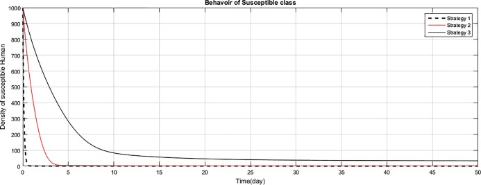
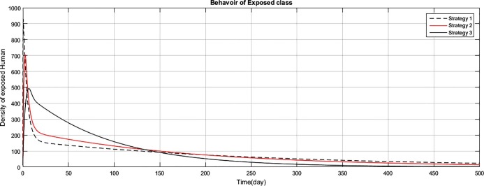
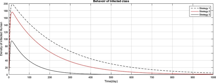
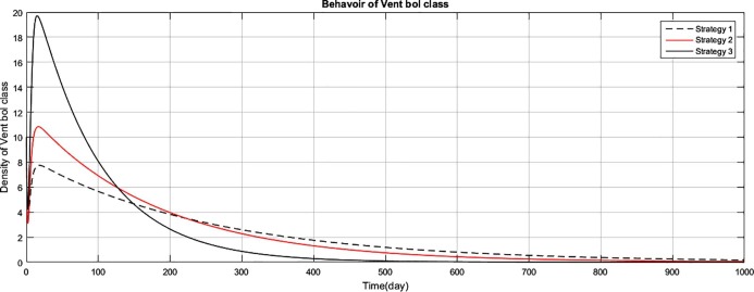
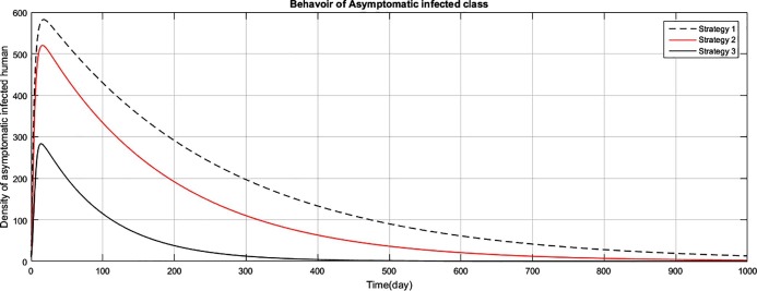
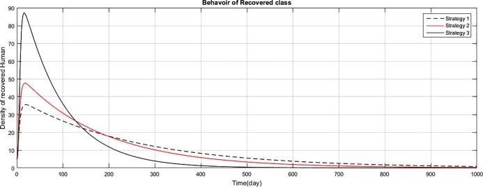
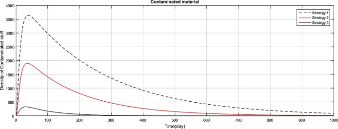
The following Fig. 1, Fig. 2 , (3), Fig. 4, Fig. 5, Fig. 6, Fig. 7 represent the results and comparison of the proposed control strategies.

Fig. 1.

The comparison of the strategies regarding maintaining the density of susceptible human population.

Fig. 2.

The graph represents the comparison of the strategies regarding exposed human population.

Fig. 3.

The graph represents the comparison of the strategies regarding infectious human population.

Fig. 4.

The graph represents the comparison of the strategies regarding the density of vent bol human population.

Fig. 5.

The graph represents the comparison of the strategies regarding asymptomatic infectious human population.

Fig. 6.

The graph represents the comparison of the strategies regarding recovered human population.

Fig. 7.

The graph represents the comparison of the strategies regarding the density of the stuff stained/shedded with corona virus.

Conclusions

In this work, a mathematical model of COVID-19 transmission and control was presented. On the basis of sensitivity indices of parameters we propose a particular combination of interventions in some particular ratio, called a strategy. We use five interventions each in transition period at $I_1,{\beta }_1$ the transmission probability of infection due to $I_1,{\beta }_2$ the transmission probability of infection due to $I_2,{\theta }_1$ the shedding coefficient of $I_1$, and ${\theta }_2$ the shedding coefficient of $I_2$. We formulate three control strategies. strategy 1 uses the actual values of the parameters with out intervention. strategy 2 and strategy 3 use the intervened values of the parameters.

The transition period of $I_1$ is intervened by giving proper treatment to the side effects of the coronavirus like throat infection, vomiting, gastrointestinal problems, nausea, diarrhea and pneumonia etc. ${\beta }_1$ is intervened by opting stay home most the time. The shedding coefficients are intervened by using face mask. ${\beta }_2$ is intervened by using sanitizer.

Fig (1) shows that implementing strategy 1 or strategy 2, the density of the susceptible human population reduces to zero. However the proposed strategy 3, maintain the density of susceptible human population constant after an initial decrease of 15 days. The exposed class plays the role of gateway in the transmission of the disease and as result of proposed strategy 3, the density of this class reduces to zero with the period of 400 days, as shown in Fig. (2) . Fig (3) shows that as result of strategy 3 the density of symptomatic infectious class reduces to zero with in a period of 450 days. Fig (4) shows that using strategy 3, we can reduce the density of vent boll class to zero with in 500 days. Increase is observed in vent bol class in the initial period of 30 days. The reason of this increase is the decrease of transition period of symptomatic infectious individuals at $I_1$. The density of asymptomatic infectious class reduces to zero with the period of 490 days, as shown in Fig (5) . As a result of strategy 3, we see in Fig. (6) that recovery increases initially for 30 days, start decreasing and reduces to zero after a period of 530 days. The reason of decrease of recovery is not the failure of strategy but the decrease in densities of the infected classes due to interventions. Greater the number of infected individuals, greater would be ratio of recovery. No doubt contaminated materials of the market play significant role in the transmission of the infection. Using strategy 3, we can eliminate this class with in period of 400 days, as shown in Fig. (7) .

Strategy 3 is recommended for complete elimination of COVID-19. Since the value of threshold, $\xi$, is less than one for the used values of parameters, so there is no chance of new outbreaks of the disease. The disease free state so obtained would be globally asymptotically stable.

Credit authorship contribution statement

Muhammad Zamir: Conceptualization, Methodology, Investigation, Visualization. Writing original draft,review, supervision & editing; F.Nadeem: Conceptualization, Methodology, Investigation, Visualization. Writing original draft,review & editing; T.Abdeljawad: Conceptualization, Methodology. Investigation Visualization, Writing original draft,review & editing; Zakia Hammouch: Conceptualization, Methodology, Investigation, Visualization, review & editing.

Declaration of Competing Interest

The authors declare that they have no known competing financial interests or personal relationships that could have appeared to influence the work reported in this paper.

References

- 1.Causes of COVID-19:https://www.mayoclinic.org/diseases-conditions/coronavirus/symptoms-causes/syc-20479963.
- 2.Myth busters: https:www.who.int novel-coronavirus-2019 advice-for-public.
- 3.WHO statement regarding cluster of pneumonia cases in Wuhan, China, Available:https://www.who.int/china/news/detail/09-01-2020.
- 4.World Health Organization. Coronavirus. World Health Organization, January 19, 2020. Available:https://www.who.int/health-topics/coronavirus.
- 5.Zhou P., Yang X.L., Wang X.G., Hu B., Zhang L., Zhang W. A pneumonia outbreak associated with a new coronavirus of probable bat origin. Nature. 2020 doi: 10.1038/s41586-020-2012-7. [DOI] [PMC free article] [PubMed] [Google Scholar]
- 6.Li Q., Guan X., Wu P., Wang X., Zhou L., Tong Y. Early transmission dynamics in Wuhan, China, of novel coronavirus-infected pneumonia. N Engl J Med. 2020 doi: 10.1056/NEJMoa2001316. [DOI] [PMC free article] [PubMed] [Google Scholar]
- 7.Coronavirus poster https:www.who.int docs coronavirus-poster-english-srilanka.
- 8.Q and A on coronaviruses (COVID-19)https://www.who.intnews-roomq-a-detailq-a-coronaviruses.
- 9.Huang C., Wang Y., Li X., Ren L., Zhao J., Hu Y. Clinical features of patients infected with 2019 novel coronavirus in Wuhan, China. Lancet. 2019;2020 doi: 10.1016/S0140-6736(20)30183-5. [DOI] [PMC free article] [PubMed] [Google Scholar]
- 10.COVID-19 CORONAVIRUS/CASES Available at:https://www.worldometers.info/coronavirus/coronavirus-cases/.
- 11.Atangana A. Modelling the spread of COVID-19 with new fractal-fractional operators: Can the lockdown save mankind before vaccination? Chaos Solitons Fractals. 2020;136 doi: 10.1016/j.chaos.2020.109860. 109860. [DOI] [PMC free article] [PubMed] [Google Scholar]
- 12.Atangana A., Araz S. Nonlinear equations with global differential and integral operators: Existence, uniqueness with application to epidemiology. Results Phys. 2020;103593 [Google Scholar]
- 13.Gao W., Baskonus H.M., Shi L. New investigation of bats-hosts-reservoir-people coronavirus model and application to 2019-nCoV system. Adv Difference Eqs. 2020;1–11 doi: 10.1186/s13662-020-02831-6. [DOI] [PMC free article] [PubMed] [Google Scholar]
- 14.Veeresha P, Prakasha DG, Malagi NS, Baskonus HM, Gao W. New dynamical behaviour of the coronavirus (COVID-19) infection system with nonlocal operator from reservoirs to people; 2020.
- 15.Media Statement: Knowing the risks for COVID-19: Available at:https://www.who.int08-03-2020-knowing-the-risk-for-covid-19.
- 16.Report of the WHO-China Joint Mission on Coronavirus Disease 2019 (COVID-19) Available at:https://www.who.intdocsdefault-sourcewho-china-joint-.
- 17.Huang C., Wang Y., Li X. Clinical features of patients infected with 2019 novel coronavirus in Wuhan, China. Lancet. 2020;395:497–506. doi: 10.1016/S0140-6736(20)30183-5. [DOI] [PMC free article] [PubMed] [Google Scholar]
- 18.Wang D, Hu B, Hu C. Clinical Characteristics of 138 Hospitalized Patients With 2019 Novel Coronavirus-Infected Pneumonia in Wuhan, China, JAMA; 2020. [DOI] [PMC free article] [PubMed]
- 19.Zhou F., Yu T., Du R. Clinical course and risk factors for mortality of adult inpatients with COVID-19 in Wuhan, China: a retrospective cohort study. Lancet. 2020 doi: 10.1016/S0140-6736(20)30566-3. [DOI] [PMC free article] [PubMed] [Google Scholar]
- 20.Pan L., Mu M., Yang P. Clinical characteristics of COVID-19 patients with digestive symptoms in Hubei, China: a descriptive, cross-sectional, multicenter study. Am J Gastroenterol. 2020 doi: 10.14309/ajg.0000000000000620. [DOI] [PMC free article] [PubMed] [Google Scholar]
- 21.https://www.scientificamerican.com/article/what-immunity-to-covid-19-really-means/.
- 22.Chan J.F., Yuan S., Kok K.H., To K.K., Chu H., Yang J. A familial cluster of pneumonia associated with the 2019 novel coronavirus indicating person-to-person transmission: a study of a family cluster. Lancet. 2019;2020 doi: 10.1016/S0140-6736(20)30154-9. [DOI] [PMC free article] [PubMed] [Google Scholar]
- 23.Zhu N., Zhang D., Wang W., Li X., Yang B., Song J. A novel coronavirus from patients with pneumonia in China, 2019. N Engl J Med. 2020 doi: 10.1056/NEJMoa2001017. [DOI] [PMC free article] [PubMed] [Google Scholar]
- 24.Bogoch I.I., Watts A., Thomas-Bachli A., Huber C., Kraemer M.U.G., Khan K. Pneumonia of unknown etiology in Wuhan, China: potential for international spread via commercial air travel. J Travel Med. 2020 doi: 10.1093/jtm/taaa008. [DOI] [PMC free article] [PubMed] [Google Scholar]
- 25.Wu J.T., Leung K., Leung G.M. Nowcasting and forecasting the potential domestic and international spread of the 2019-nCoV outbreak originating in Wuhan, China: a modelling study. Lancet. 2020 doi: 10.1016/S0140-6736(20)30260-9. [DOI] [PMC free article] [PubMed] [Google Scholar]
- 26.Zhao S., Lin Q., Ran J., Musa S.S., Yang G., Wang W. Preliminary estimation of the basic reproduction number of novel coronavirus (2019-nCoV) in China, from 2019 to 2020: a data-driven analysis in the early phase of the outbreak. Int J Infect Dis. 2020 doi: 10.1016/j.ijid.2020.01.050. [DOI] [PMC free article] [PubMed] [Google Scholar]
- 27.Zhao S., Musa S.S., Lin Q., Ran J., Yang G., Wang W. Estimating the unreported number of novel coronavirus (2019-nCoV) cases in China in the first half of January 2020: a data-driven Modelling analysis of the early outbreak. J Clin Med. January 2020;2020 doi: 10.3390/jcm9020388. [DOI] [PMC free article] [PubMed] [Google Scholar]
- 28.Chen T.M., Rui J., Wang Q.P., Zhao Z.Y., Cui J.A., Yin L. Amathematical model for simulating the phase-based transmissibility of a novel coronavirus. Infectious Diseases Poverty. 2020;9(4) doi: 10.1186/s40249-020-00640-3. [DOI] [PMC free article] [PubMed] [Google Scholar]
- 29.Ivorra B., Ferrandez M.R., Vela-Perez M., Ramos A.M. Mathematical modeling of the spread of the coronavirus disease 2019, (COVID-19) considering its particular characteristics. The case of China. 2020;MOMAT,1–23 doi: 10.13140/RG.2.2.21543.29604. [DOI] [PMC free article] [PubMed] [Google Scholar]
- 30.Yang C., Wang J. A mathematical model for the novel coronavirus epidemic in Wuhan, China. Math Biosci Eng. 2020;17(3):2708–2724. doi: 10.3934/mbe.2020148. [DOI] [PMC free article] [PubMed] [Google Scholar]
- 31.Spencer JA, Shutt DP, Moser SK, Clegg H, Wearing HJ, Mukundan H, et al. Epidemiological parameter review and comparative dynamics of influenza, respiratory syncytial virus,rhinovirus, human coronvirus, and adenovirus, medRxiv; 2020.
- 32.Report of the WHO-China Joint Mission on Coronavirus Disease 2019 (COVID-19.)https://www.who.int/docs/default-source/coronaviruse/who-china-joint-mission-on-covid-19-final-report.pdf.
- 33.Nadeem F., Zamir M., Tridane A., Khan Y. Modeling and Control of Zoonotic Cutaneous Leishmaniasis. J Math. 2019;51(2):105–121. ISSN 1016-2526. [Google Scholar]
- 34.Desjeuk P. Leishmaniasis: current situation and new perspective. Comparative Immunology Microbiology and Infectious Disease. 2004;27(5):305–318. doi: 10.1016/j.cimid.2004.03.004. [DOI] [PubMed] [Google Scholar]
- 35.Zamir M., Sultana R., Ali R., Panhwar W.A., Kumar S. Study on the threshold condition for infection of visceral leishmaniasis. Sindh Univ Res J (Sci Ser) 2015;47(3):619–622. [Google Scholar]
- 36.https://www.webmd.com/lung/qa/what-percentage-of-covid19-cases-are-mild.
- 37.https://www.theguardian.com/society/2020/mar/28/coronavirus-intensive-care-uk-patients-50-per-sent-survival-rate.
- 38.Wu Z., McGoogan J.M. Characteristics of and Important Lessons From the Coronavirus Disease 2019 (COVID-19) Outbreak in China: Summary of a Report of 72314 Cases From the Chinese Center for Disease Control and Prevention. JAMA. 2020 doi: 10.1001/jama.2020.2648. [DOI] [PubMed] [Google Scholar]
- 39.Lavezzo E, Franchin E, Ciavarella C. Suppression of COVID-19 outbreak in the municipality of Vo’, Italy. available herehttps://www.medrxiv.org/content/10.1101/2020.04.17.20053157v1.full.pdf.
- 40.Covid-19: four fifths of cases are asymptomatic, China figures indicate. BMJ2020;369 doi: 10.1136/bmj.m1375. [DOI] [PubMed]
- 41.Ngoteya F.N., Gyekye Y.N. Sensitivity analysis of parameters in a competition model. Appl Comput Math. 2015;4(5):363–368. [Google Scholar]
- 42.Kamgang J.C., Sallet G. Computation of threshold conditions for epidemiological models and global stability of the disease-free equilibrium. Math Biosci. 2008;213:1–12. doi: 10.1016/j.mbs.2008.02.005. [DOI] [PubMed] [Google Scholar]
- 43.Sundar S., Agrawal G., Rai M., Makharia M.K., Murray H.W. Treatment of Indian visceral leishmaniasis with single or daily infusion of low dose liposomal amphotericin, Randomised trial. BMJ. 2001;323:419–422. doi: 10.1136/bmj.323.7310.419. [DOI] [PMC free article] [PubMed] [Google Scholar]
- 44.Zamir M., Shah Z., Nadeem F., Memood A., Alrabaiah H., Kumam P. Non pharmaceutical interventions for optimal control of COVID-19. Comput Methods Programs Biomed. 2020;196:105642. doi: 10.1016/j.cmpb.2020.105642. ISSN 0169–2607. [DOI] [PMC free article] [PubMed] [Google Scholar]
- 45.Zamir M., Nadeem F., Zaman G. Optimal control of visceral, cutaneous and post kala azar leishmaniasis. Adv Difference Eqs. 2020:548. doi: 10.1186/s13662-020-02979-1. [DOI] [Google Scholar]