CT IMAGE RECONSTRUCTION ON A LOW DIMENSIONAL MANIFOLD

Abstract

The patch manifold of a natural image has a low dimensional structure and accommodates rich structural information. Inspired by the recent work of the low-dimensional manifold model (LDMM), we apply the LDMM for regularizing X-ray computed tomography (CT) image reconstruction. This proposed method recovers detailed structural information of images, significantly enhancing spatial and contrast resolution of CT images. Both numerically simulated data and clinically experimental data are used to evaluate the proposed method. The comparative studies are also performed over the simultaneous algebraic reconstruction technique (SART) incorporated the total variation (TV) regularization to demonstrate the merits of the proposed method. Results indicate that the LDMM-based method enables a more accurate image reconstruction with high fidelity and contrast resolution.

1. Introduction.

X-ray computed tomography (CT) is a major imaging modality in medical, security, and industrial applications. The filtered back-projection (FBP) is an efficient and robust method for x-ray CT image reconstruction [10], but it generates strong noise and artifacts in the cases of low-dose or incomplete datasets. Extensive efforts have been made to improve image quality for practical purposes [9, 19, 6]. Iterative methods incorporate prior information of images, and offer distinct advantages over the analytic methods in cases of noisy and few-view data. The statistical iterative methods model the statistics of photons to improve the reconstructed image quality from the low-dose acquisitions [6, 20]. Recently, the compressive sensing (CS) approach [3, 4] is applied for the image reconstruction from less measurements than that required by the Nyquist-Shannon sampling theorem. Based on the CS theory, image reconstruction algorithms were developed for various problems of CT image reconstruction to improve image quality and reduce radiation dose, such as total variation (TV) regularization [19, 20], prior image constrained compressed sensing (PICCS) [5], nonlocal mean (NLM) [1, 9], and dictionary learning (DL) [21]. TV is a typical sparse transform for an image, and is a popular regularization form for image reconstruction due to its ability to preserve image edges. However, it is effective only for reconstruction of piecewise constant images and would over-smoothen textured regions, which may sacrifice important details. PICSS could be seen as a generalization of the TV regularization method. It incorporates a preliminary reconstructed image into CS reconstruction technique to achieve more accurate image reconstruction [5]. NLM exploits a high degree of redundancy of an image for de-noising [1]. The similarity is derived from intensity differences between neighboring patches of pixels or voxels. A non-linear filter can be used to reduce image noise by updating each pixel value with a weighted average of its neighbors according to the similarity of involved patches. DL builds adaptive sparse representation elements from a training set of images, and utilizes domain knowledge at a deeper level [21]. The dictionary tends to capture local image features effectively and helps image denoising and feature inference. However, the structural differences between a true image and training images could affect the image reconstruction quality.

The idea of the proposed X-ray CT image reconstruction method is inspired by a recent method called the low-dimensional manifold model (LDMM) [14, 16]. Using the image patches discussed in nonlocal methods [2], the LDMM interprets image patches as a point cloud sampled in a low-dimensional manifold embedded in a high dimensional ambient space, which provides a new way of regularization by minimizing the dimension of the corresponding image patch manifold. This can be explained as a natural extension of the idea of low-rank regularization for linear objects to data with more complicated structures [7]. Moreover, the authors in [14] elegantly find that the point-wisely defined manifold dimension can be computed as a Dirichlet energy of the coordinate functions on the manifold, whose corresponding boundary value problem can be further solved by a point integral method proposed in [14]. The LDMM performs very well in image imprinting and super-resolution. The patch manifold of images is generally a low dimensional structure, and accommodates rich structural information [16]. With the LDMM prior knowledge on images, this proposed method significantly enhances contrast resolution of image reconstruction.

In this paper, LDMM-based regularization method is proposed for CT image reconstruction. The LDMM-based reconstruction method is to maximize the data fidelity and minimize the manifold dimensionality, which is performed using the Bregman iteration [15] by updating the patch manifold structure iteratively. By a standard variational approach, the regularization model of image reconstruction can be reduced to the Laplace-Beltrami equations over a point cloud, which is solved using the point integral method [11].

The rest of the paper is organized as follows. In section 2, we provide a detailed description for the CT image reconstruction based on LDMM. A numerical reconstruction algorithm is presented based on Bregman iteration. In section 3, we perform the image reconstruction using numerical simulation data and the clinical raw projection data to evaluate the proposed LDMM-based image reconstruction method. In addition, we also conduct comparative studies with popular simultaneous algebraic reconstruction technique (SART) with TV method to present the merits of the proposed method. After that, we conclude the paper in the last section.

2. Image reconstruction method.

In this section, we first review the statistical model of x-ray CT imaging. After that, we discuss the proposed method of CT image reconstruction based on LDMM and its numerical algorithm.

2.1. Statistical model for X-ray CT imaging.

In x-ray CT imaging, the number ξ of x-ray photons recorded by a detector element is a random variable, which obeys a Poisson distribution [10]:

$$p\left(\xi =y_i\right)=\frac{{\overline{y}}^{y_i}}{y_i!}\text{exp}\left(-{\overline{y}}_i\right)$$ (1)

The expectation value of x-ray photons along a path ℓ from x-ray source to i-th detector element obeys Beer-Lambert law:

$${\overline{y}}_i=b_i\text{exp}\left(-{\int }_{\ell }\mathit{\mu }(\overrightarrow{r})\text{d}\ell \right)$$ (2)

where b_i is the number of x-ray photons detected by i-th detector element in the blank scanning (without any object in the beam path), and $\mathit{\mu }\left(\overrightarrow{r}\right)$ is the linear attenuation coefficient of the object. To implement the numerical computation, Eq. (2) can be discretized as,

$${\overline{y}}_i=b_i\text{exp}\left(-{\mathit{A}}_i\mathit{\mu }\right)$$ (3)

where μ is a vector composed of pixel values on image of linear attenuation coefficients, and A_i is the weighting coefficients of the pixel values on i-th beam path. Since data are independent between detectors, the likelihood function for x-ray photons probability distribution on detectors is defined by,

$$P(\mathit{Y}\mid \mathit{\mu })=\prod _{i=1}^N\frac{{\overline{y}}^{y_i}}{y_i!}\text{exp}\left(-{\overline{y}}_i\right)$$ (4)

where Y = (y₁, y₂, ⋯, y_N)^T. According to the Bayesian rule: p(μ|Y)p(Y) = (Y|μ)p(μ), the image reconstruction task can be implemented by maximizing a posteriori (MAP) distribution p(μ|Y), which is equivalent to the following minimization problem in term of the monotonic property of the natural logarithm [20, 12]:

$$\mathit{\mu }=\text{arg}\text{min}\left(\sum _{i=1}^N\left[{\overline{y}}_i-y_i\text{log}\left({\overline{y}}_i\right)\right]+R(\mathit{\mu })\right)$$ (5)

where r(μ) = −ln(p(μ)) is a regularization term expressing the prior knowledge about the attenuation image μ , and N is the total number of x-ray beam paths. In the context, we propose to use the low-dimension of an image as prior knowledge to conduct the image reconstruction, which is discussed in the next section. After inserting Eq. (3) in Eq. (5), a second-order approximation is applied to simplify the complicated optimization to a quadratic optimization:

$$\mathit{\mu }=\text{arg}\text{min}\left[\sum _{i=1}^N\frac{b_i}{2}{\left({\mathit{A}}_i\mathit{\mu }-y_i\right)}^2+R(\mathit{\mu })\right]$$ (6)

2.2. Image reconstruction based on LDMM.

The classical image restoration models mainly focus on local properties of the objective image, such as smoothness and jumps. Image features can be further enhanced due to its possible repetitive patterns non-locally. The nonlocal based image restoration methods [2] extract and match non-local repetitive structures of images using image patches. An essential observation of nonlocal methods is that images can be restored by enhancing similar patterns which may not lie in nearby regions of the original image domain. Therefore, comparing with the direct regularization methods on the image domain, the quality of image restoration can be usually improved using nonlocal methods. For instance, nonlocal based variational methods [2, 8, 22] and nonlocal based wavelet frame based methods demonstrate outstanding image restoration results [17].

Let μ denote an image containing m × n pixels: μ = {μ(i, j) | 1 ≤ i ≤ m, 1 ≤ j ≤ n} , and ${\mathcal{P}}_{\left(i_0,j_0\right)}(I)$ denotes an image patch centering at (i₀, j₀) with size of 2s₁s₂, namely, ${\mathcal{P}}_{\left(i_0,j_0\right)}(I)=\left\{I(i,j)\mid i_0-s_1\le i<i_0+s,j_0-s_2\le j<j_0+s_2\right\}$. An image is decomposed into a set of patches. These patches can be overlapping or nonoverlapping. Let $\mathcal{P}(\mathit{\mu })$ denote the patch transformation which maps any given image I to be the set of image patches. $\mathcal{P}(\mathit{\mu })$ can be also viewed as a point set in ${ℝ}^d$ with a dimension of d = 2s₁ × s₂ . It samples a low dimensional manifold $\mathcal{M}(\mathit{\mu })$ embedded in ${ℝ}^d$, which is called the patch manifold of μ [14, 16]. The patch manifold is low dimensional for many natural images, such as X-ray CT images. A patch manifold can be constructed directly from an image using patching size 2s₁ × 2s₂. As an example illustrated in the right image of Fig. 1, we construct a patch manifold of a CT image using patching size 16 × 16 and color-code its piecewise dimension on the image to show the variation of the manifold dimension. More recently, [14] proposes to regularize the dimension of the patch manifold $\mathcal{M}(\mathit{\mu })$ for image restoration. Inspired by [14], we use the dimension of the patch manifold as a regularization term to seek the dimension of its patch manifold as small as possible such that detail structure information can be magnified for the CT image reconstruction. Therefore, the optimization model Eq. (6) is reformulated for the measurement data fidelity and the manifold dimensional quantification:

$$\mathit{\mu }=\text{arg}\underset{\mathit{\mu }}{\text{min}}\left[\frac{\lambda }{2}\sum _{i=1}^N{b}_i{\left({\mathit{A}}_i\mathit{\mu }-y_i\right)}^2+{\int }_{\mathcal{M}}\text{dim}(\mathcal{M}(\mathit{\mu }))(\mathit{x})\text{d}\mathit{x}\right]$$ (7)

where $\text{dim}(\mathcal{M}(\mathit{\mu }))(\mathit{x})$ denotes the dimension of the patch manifold $\mathcal{M}(\mathit{\mu })$ of an image μ at x, a point in $\mathcal{M}(\mathit{\mu })\subset {ℝ}^d$. The patch manifold of a nature image may be a set of several manifolds with different dimensions, corresponding to different patterns of the image. In [14], the authors elegantly demonstrate that the dimension of the patch manifold for an image μ at given patch x can be calculated by the coordinate function,

$$\mathit{\text{dim}}(\mathcal{M}(\mathit{\mu }))(\mathit{x})=\sum _{i=1}^d{\left|{\nabla }_{\mathcal{M}}{\alpha }_i(\mathit{x})\right|}^2$$ (8)

where α_i is the embedding coordinate function defined by α_i(x) = x_i for any $\mathit{x}=\left(x_1,x_2,\cdots ,x_d\right)\in \mathcal{M}\subset {ℝ}^d$. Combining Eqs. (7) and (8), we obtain

$$\text{arg}\underset{\mathit{\mu },\mathcal{M}\subset {ℝ}^d}{\text{min}}\left[\frac{\lambda }{2}\sum _{i=1}^N{b}_i{\left({\mathit{A}}_i\mathit{\mu }-y_i\right)}^2+\sum _{i=1}^d{\Vert {\nabla }_{\mathcal{M}}{\alpha }_i(x)\Vert }_{L^2(\mathcal{M})}^2\right],\hspace{1em}\text{s}.\text{t}.\mathcal{P}(\mathit{\mu })\subset \mathcal{M}$$ (9)

where $\mathcal{M}$ is a manifold embedded in ${ℝ}^d$, and $\mathcal{P}(\mathit{\mu })$ is the patch set of image μ. Note that the dimension formula (8) holds point-wisely for the embedding manifolds. The above regularization is actually the L₁ norm of the local dimension. The optimization (9) can be solved by alternating direction method similar as the one proposed in [14]. In other words, given an estimation of the manifold ${\mathcal{M}}^n$ and an estimation of image μⁿ satisfying $\mathcal{P}\left({\mathit{\mu }}^n\right)\subset {\mathcal{M}}^n$, the coordinate functions α = {α_i} and an updated image μ are computed through the following optimization.

$$\text{arg}\underset{\mathit{\mu },\mathbf{\alpha }}{\text{min}}\left[\frac{\lambda }{2}\sum _{i=1}^N{b}_i{\left({\mathit{A}}_i\mathit{\mu }-y_i\right)}^2+\sum _{i=1}^d{\Vert {\nabla }_{\mathcal{M}}{\alpha }_i(x)\Vert }_{L^2(\mathcal{M})}^2\right],\hspace{1em}\text{s}.\text{t}.\mathit{\alpha }\left(\mathcal{P}\left({\mathit{\mu }}^n\right)\right)=\mathcal{P}(\mathit{\mu })$$ (10)

From the reconstructed coordinates α, the manifold $\mathcal{M}$ is further updated by ${\mathcal{M}}^{n+1}=\left\{\left({\alpha }_1(x),\cdots ,{\alpha }_d(x)\right)\mid x\in {\mathcal{M}}^n\right\}$. This process is iterated until convergence of iterative procedure. Given the manifold $\mathcal{M}$, the optimization problem (10) can be solved to compute the coordinate functions α_i(i = 1, 2, …, d) and update the image μ using the Bregman iteration [15]. Mathematically, we have:

$${\mathit{\alpha }}^{n+1,k+1}=\text{arg}\underset{\mathit{\alpha }}{\text{min}}\left[\sum _{i=1}^d{\Vert {\nabla }_{{\mathcal{M}}^n}{\mathit{\alpha }}_i(x)\Vert }_{L^2\left({\mathcal{M}}^n\right)}^2+\beta {\Vert \mathit{\alpha }\left(\mathcal{P}\left({\mathit{\mu }}^n\right)\right)-\mathcal{P}\left({\mathit{\mu }}^{n+1,k}\right)+Q^k\Vert }_F^2\right]$$ (11a)

$${\mathit{\mu }}^{n+1,k+1}=\text{arg}\underset{\mathit{\mu }}{\text{min}}\left[\frac{\lambda }{2}\sum _{i=1}^N{b}_i{\left({\mathit{A}}_i\mathit{\mu }-y_i\right)}^2+\beta {\Vert {\mathit{\alpha }}^{k+1}\left(\mathcal{P}\left({\mathit{\mu }}^n\right)\right)-\mathcal{P}(\mathit{\mu })+Q^k\Vert }_F^2\right]$$ (11b)

$$Q^{k+1}=Q^k+{\mathit{\alpha }}^{n+1,k+1}\left(\mathcal{P}\left({\mathit{\mu }}^n\right)\right)-\mathcal{P}\left({\mathit{\mu }}^{k+1}\right)$$ (11c)

where $\mathit{\alpha }(\mathcal{P}(\mathit{\mu }))={\left({\alpha }_1(\mathcal{P}(\mathit{\mu })),\cdots ,{\alpha }_d(\mathcal{P}(\mathit{\mu }))\right)}^T$. In the Bregman iteration, Eq. (11b) can be reduced to a qudratic minimization, which can be solved using the conjugate gradient (CG) method to produce the exact solution after a finite number of iterations. The optimization (11a) can be solved for each coordinate function α_i(i = 1, …, d) separately. Applying the standard variation method, Eq. (11a) is equivalent to solving following Laplace-Beltrami equation.

$$\{\begin{array}{cc}-{\Delta }_{\mathcal{M}}u(\mathit{x})+\beta {\sum }_{y\in \Omega }\delta (\mathit{x}-\mathit{y})(u(\mathit{y})-v(\mathit{y}))=0,& \mathit{x}\in \mathcal{M}\\ \frac{\partial u}{\partial \overrightarrow{n}}(\mathit{x})=0,& \mathit{x}\in \partial \mathcal{M}\end{array}$$ (12)

where $\mathcal{M}={\mathcal{M}}^n$, u represents any α_i, $\overrightarrow{n}$ is the out normal of $\mathcal{M}$ with the boundary $\partial \mathcal{M}$ and $\Omega =\mathcal{P}\left({\mathit{\mu }}^n\right)$. Recently, the point integral method has been proposed to solve Laplace-Beltrami equation over a point cloud [3]. The main idea of the point integral method is to apply following integral approximation for the differential term in Laplace-Beltrami equation:

$${\int }_{\mathcal{M}}{\Delta }_{\mathcal{M}}u(\mathit{y})R_t(\mathit{x},\mathit{y})\text{d}y\approx -\frac{1}{t}{\int }_{\mathcal{M}}(u(\mathit{x})-u(\mathit{y}))R_t(\mathit{x},\mathit{y})\text{d}\mathit{y}+2{\int }_{\partial \mathcal{M}}\frac{\partial u(\mathit{y})}{\partial \overrightarrow{n}}{R}_t(\mathit{x},\mathit{y})\text{d}\mathit{y}$$ (13)

where R_t(x, y) are kernel functions given as follows,

$$R_t(\mathit{x},\mathit{y})=C_t\mathit{\text{exp}}\left(-\frac{\Vert \mathit{x}-\mathit{y}{\Vert }^2}{4t}\right)$$ (14)

where C_t is a normalizing factor. Using the integral approximation (13), following integral equation can be obtained to approximate the Laplace-Beltrami equation,

$${\int }_M(u(\mathit{x})-u(\mathit{y}))R_t(\mathit{x},\mathit{y})\text{d}\mathit{y}+t\beta \sum _{\mathit{y}\in \Omega }{R}_t(x,y)(u(\mathit{y})-u(\mathit{y}))=0$$ (15)

The integral equation (15) can be further discretized into a matrix equation over the point set using quadrature rule [14]:

$$\{\begin{array}{c}(\mathit{L}+\overline{\beta }\mathit{W})U=\overline{\beta }\mathit{W}\mathit{V}\\ \mathit{L}=\mathit{D}-\mathit{W}\end{array}$$ (16)

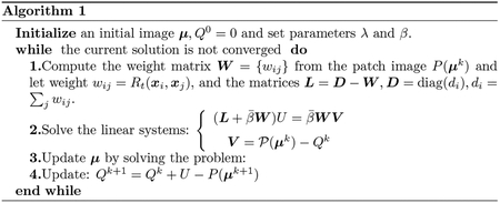
where $\overline{\beta }=\frac{tN\beta }{\left|\mathcal{M}\right|}$, W = (R_t(x_i, x_j))_{i, j=1, …, N} is the weight matrix, $\mathit{D}=\text{diag}\left({\left\{\sum _j{w}_{ij}\right\}}_{1,\cdots ,N}\right)$ and $\mathit{V}=\mathcal{P}\left({\mathit{\mu }}^k\right)-Q^k$. Thus, the optimization (11a) can be solved based on the matrix equation (16). The detailed formulation and alternating minimization steps for solving Eq. (10) are described in the flowchart for Algorithm 1.

Figure 1.

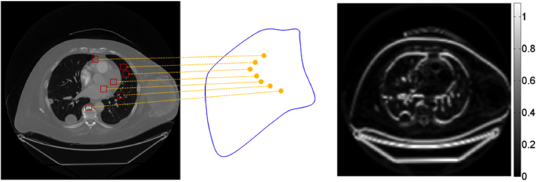
The patch manifold of a CT image (left) and the corresponding dimension function of the patch manifold with patch size 16 × 16 (right).

3. Numerical experiments.

In the section, we test the proposed LDMM-based reconstruction method with numerical simulation and real experimental datasets obtained on a GE clinical CT scanner. We constructed a patch manifold of an image with a patch size of 1616 by shifting 8 pixels. In addition, we also perform the comparative studies with the state of the art method, the simultaneous algebraic reconstruction technique (SART) with a total variation (TV) [18], to demonstrate the merits of the proposed method. All numerical computations in this section are implemented by MATLAB in a PC with 16G RAM and 2.8GHz CPU.

3.1. Simulation data.

A phantom was adapted from a CT slice to evaluate the proposed algorithms. Data acquisitions are simulated with polychromatic x-ray source operated at 120 kVp/5mAs dose for the x-ray imaging. The radius of the scanning trajectory was 53.852cm. The source-to-detector distance was 94.6746 cm. 540 projections are uniformly acquired over a 360-degree angular range. 765 detector elements are equiangular distributed on each projection view. The phantom is discretized into a 512 × 512 matrix. We choose the regularization parameters as λ = 0.3 and β = 0.15. The x-ray imaging process was simulated to generate projection data according to the x-ray propagation forward model, the polychromatic Beer-Lambert law. The projection datasets were corrupted by Poisson noise to simulate real x-ray imaging experiments. We performed the image reconstruction using the proposed LDMM-based image reconstruction and the simultaneous algebraic reconstruction technique (SART) with a total variation (TV), respectively. Results show that the LDMM-based method is able to produce more accurate image reconstruction with high fidelity and detailed features than the SART+TV method that would over-smoothen textural pattern in reconstructed image. We calculated the peak-to-noise ratio (PSNR) and structural similarity (SSIM) for the reconstructed image, and obtained PSNR of 52.42 and SSIM of 0.9940 for the LDMM-based reconstruction, and PSNR of 39.53 and SSIM of 0.9911 for the SART+TV method. Fig. 2 shows a comparison between the reconstructed images and the ground truth. Fig. 3 presents the comparison of profiles along the horizotal and vertical midlines in the phantom and reconstructed images.

Figure 2.

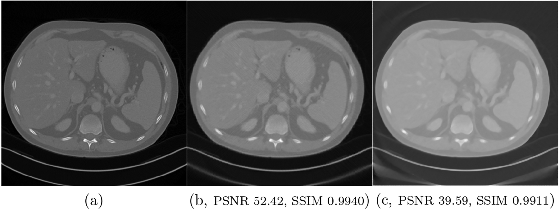
Comparison of image reconstruction. (a) Ground truth CT images, (b) the reconstructed image using the LDMM-based method, and (c) the reconstructed image using SART with TV.

Figure 3.

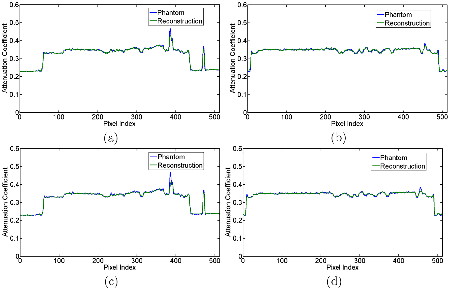
Profiles of reconstructed image. (a) The profiles along the vertical midlines in the phantom and image reconstructed by LDMM-based reconstruction method, (b) the profiles along the horizontal midlines in the phantom and image reconstructed by LDMM-based reconstruction method. (c) The profiles along the vertical midlines in the phantom and image reconstructed by SART+TV reconstruction method, and (d) the profiles along the horizontal vertical midlines in the phantom and image reconstructed by SART+TV reconstruction method.

3.2. Low dose data.

A realistic phantom adapted from a human CT slice is used to evaluate the proposed algorithms. We use an computer-assisted tomography simulation (CatSim) software [13], which was developed by GE Global Research Center, to simulate x-ray imaging for the phantom. CatSim incorporates polychromaticity, realistic quantum and electronic noise models, finite focal spot size and shape, finite detector cell size, and detector cross-talk for the simulation of real x-ray imaging. All acquisitions are simulated with polychromatic x-ray source operated at 120 kVp and 0.2mSv dose for the low dose x-ray imaging. The radius of the scanning trajectory is 54.1cm. Source-to-detector distance is 94.9cm. 888 detector elements are equiangular distributed on each projection view. 984 projections are uniformly acquired over a 360-degree angular range, generating the sinogram, as shown in Fig. 6. The phantom is discretized into a 512 × 512 matrix. We choose the regularization parameters as λ = 0.3 and β = 0.3. We performed the image reconstruction respectively using the proposed LDMM-based image reconstruction and SART +TV, which achieve PSNR of 18.72 and SSIM of 0.79 for the LDMM-based reconstruction method, and PSNR of 18.69 and SSIM of 0.74 for the SART+TV method. Results show that the LDMM-based image reconstruction method had a better contrast resolution of the reconstructed image than the SART+TV method, as shown in Fig. 5.

Figure 6.

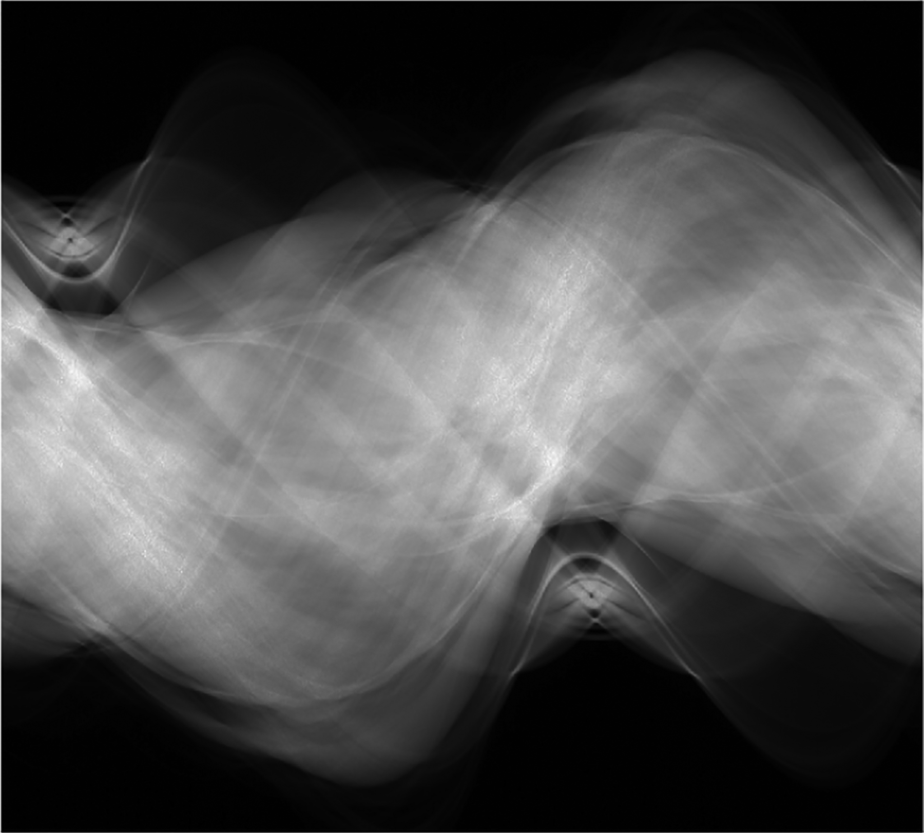
The sinogram measured from a clinical x-ray CT scanner.

Figure 5.

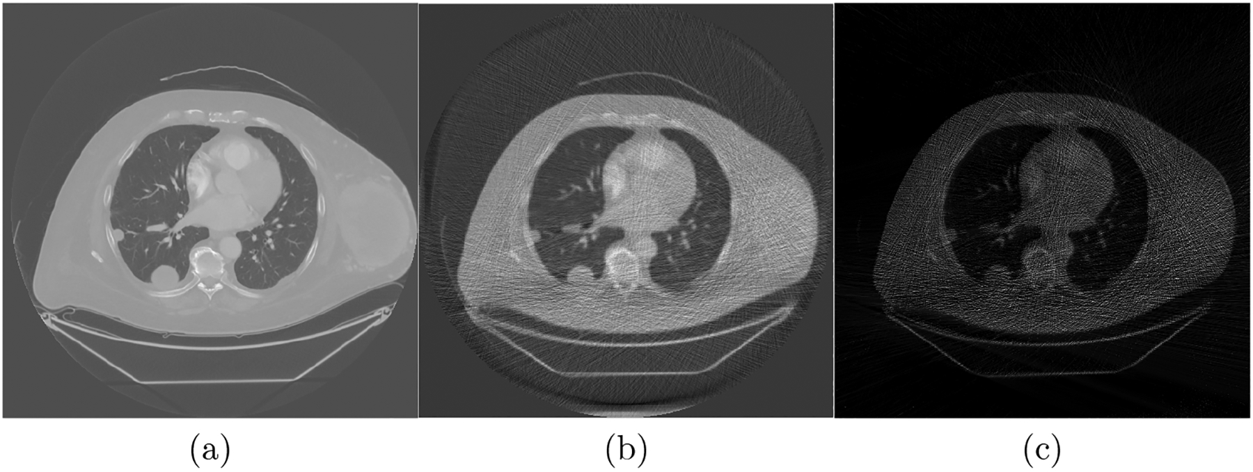
Comparison of CT reconstruction. (a) Ground truth CT images, (b) the reconstructed image using the LDMM-based image reconstruction method, and (c) the reconstructed image using SART with TV.

3.3. Clinical data.

A clinical CT raw projection dataset obtained from GE Healthcare was used to evaluate the LDMM-based image reconstruction method. After appropriate preprocessing for the projection data, we obtained a set of fanbeam sinogram, as shown in Fig. 6. In the x-ray imaging, the field of view (FOV) is of a 25 cm radius, and the radius of the scanning trajectory is 54.1cm. Source-to-detector distance is 94.9cm. 984 projections are uniformly acquired over a 360-degree angular range. 888 detector elements with 1.024mm pitch were equiangular distributed on a projection view. The image matrix was of 512 × 512 pixels. We choose the regularization parameters as λ = 0.2 and β = 0.5. We conducted the image reconstruction from the sinogram using the proposed LDMM-based reconstruction method. For comparison, the FBP method and the SART with TV regularization were applied as well to perform the image reconstruction from same projection dataset. Results show that the LDMM-based image reconstruction out-performs the other two reconstruction methods, as shown in Fig. 7. The LDMM-based method well preserves structural information especially texture features of the reconstructed image. The SART with TV iteration method was suitable to reconstruct high contrast images, whereas it would over-smoothen textured regions in medical images, resulting in the loss of details. FBP keeps the structural information, but it produced noisy image.

Figure 7.

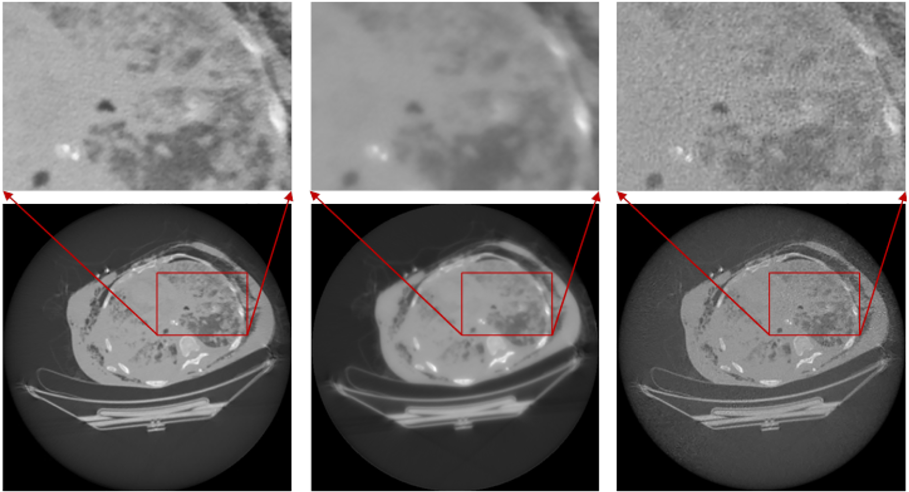
Comparison of CT image reconstructions from clinical CT raw data. (a) The reconstructed image using the LDMM-based method, (b) the reconstructed image using SART with TV, and (c) the reconstructed image using FPB.

4. Discussions and conclusion.

The major contribution in this paper is to propose an image reconstruction method aided by the regularization of a low dimensional manifold model (LDMM). The patch manifold of a natural image is generally with a low dimensional structure, and accommodates rich structural information. LDMM regularization method well recovers structural information of images, and promises substantially to increase spatial and contrast resolution of the image reconstruction. The comparison between the proposed method and the representative the SART with TV methods has been performed to illustrate the merits of the LDMM-based reconstruction approach. The raw datasets from a clinical CT scanner have been used to evaluate the performance of the image reconstruction methods. Results show that the regularization method of low dimensional manifold is an efficient and robust image reconstruction technique, and well preserves image edges and structural details of the reconstructed image comparing to the state of the art SART with TV image reconstruction. The iterative algorithm also incorporates prior knowledge, and account for photon statistics at a low dose level. Major computational cost is matrix-vector multiplication operations in the LDMM-based image reconstruction. Because matrix-vector multiplication is well computed parallel, the computational speed of the proposed iterative method can be significantly improved by parallel programming. This LDMM-based image reconstruction approach is very promising for medical imaging and other applications.

Figure 4.

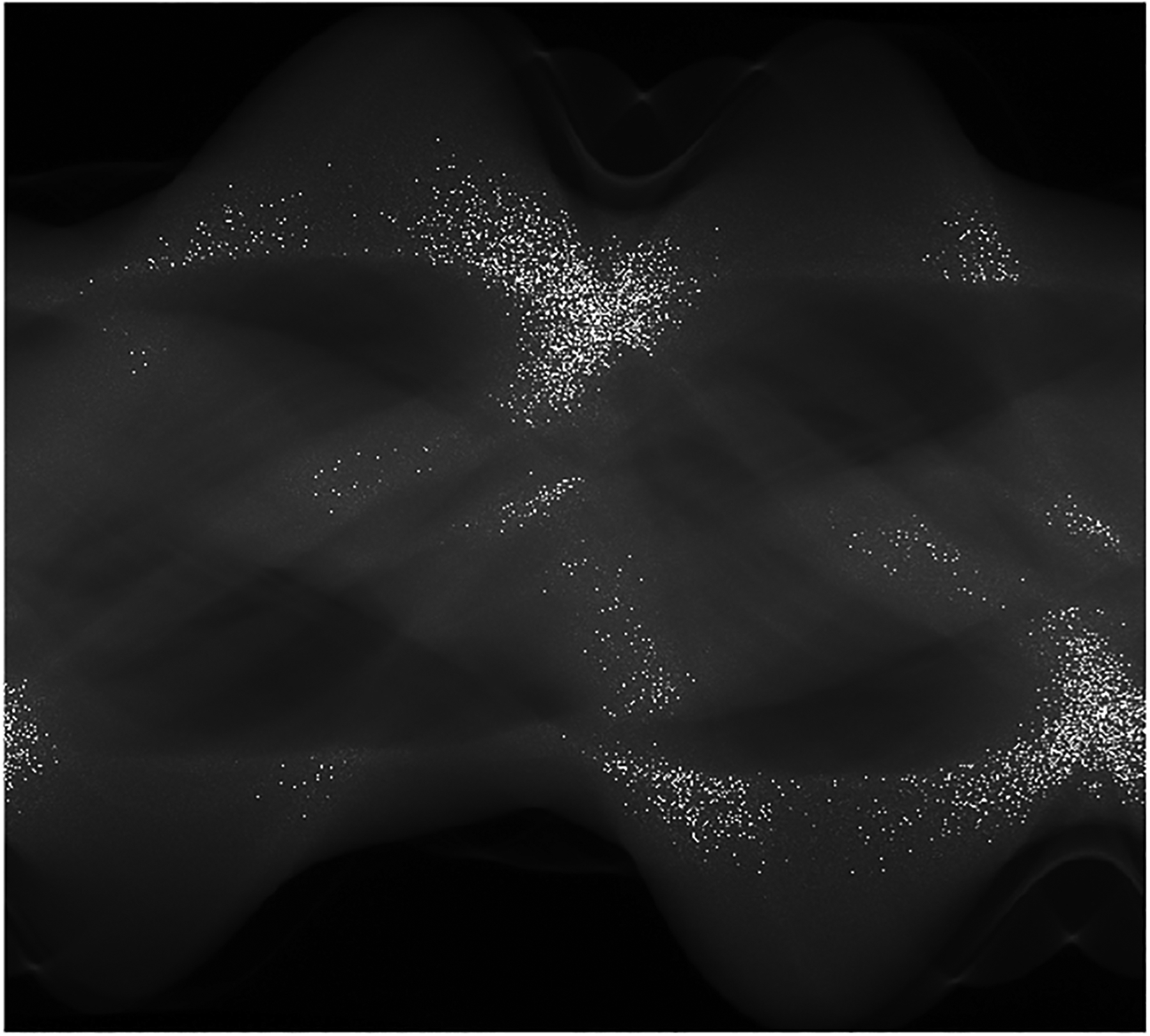
The sinogram simulated from CatSim.

REFERENCES

- [1].Brox T, Kleinschmidt O and Cremers D, Efficient nonlocal means for denoising of textural patterns, IEEE Transactions on Image Processing, 17 (2008), 1083–1092. [DOI] [PubMed] [Google Scholar]
- [2].Buades A, Coll B and Morel J-M, A non-local algorithm for image denoising, In Computer Vision and Pattern Recognition, 2005. CVPR 2005. IEEE Computer Society Conference on, volume 2, pages 60–65. IEEE, 2005. [Google Scholar]
- [3].Candès EJ, Romberg J and Tao T, Robust uncertainty principles: Exact signal reconstruction from highly incomplete frequency information, IEEE Transactions on Information Theory, 52 (2006), 489–509. [Google Scholar]
- [4].Candes EJ, Romberg JK and Tao T, Stable signal recovery from incomplete and inaccurate measurements, Communications on Pure and Applied Mathematics: A Journal Issued by the Courant Institute of Mathematical Sciences, 59 (2006), 1207–1223. [Google Scholar]
- [5].Chen G-H, Tang J and Leng S, Prior image constrained compressed sensing (piccs): a method to accurately reconstruct dynamic ct images from highly undersampled projection data sets, Medical Physics, 35 (2008), 660–663. [DOI] [PMC free article] [PubMed] [Google Scholar]
- [6].Elbakri IA and Fessler JA, Statistical image reconstruction for polyenergetic x-ray computed tomography, IEEE Transactions on Medical Imaging, 21 (2002), 89–99. [DOI] [PubMed] [Google Scholar]
- [7].Gao H, Yu H, Osher S and Wang G, Multi-energy ct based on a prior rank, intensity and sparsity model (prism), Inverse Problems, 27 (2011), 115012, 22pp. [DOI] [PMC free article] [PubMed] [Google Scholar]
- [8].Gilboa G and Osher S, Nonlocal operators with applications to image processing, Multiscale Modeling & Simulation, 7 (2008), 1005–1028. [Google Scholar]
- [9].Ha S and Mueller K, Low dose ct image restoration using a database of image patches, Physics in Medicine & Biology, 60 (2015), 869–882. [DOI] [PubMed] [Google Scholar]
- [10].Kak AC and Slaney M, Principles of Computerized Tomographic Imaging, IEEE press; New York, 1988. [Google Scholar]
- [11].Li Z, Shi Z and Sun J, Point integral method for solving poisson-type equations on manifolds from point clouds with convergence guarantees, Communications in Computational Physics, 22 (2017), 228–258. [Google Scholar]
- [12].De Man B, Nuyts J, Dupont P, Marchal G and Suetens P, An iterative maximum-likelihood polychromatic algorithm for ct, IEEE Transactions on Medical Imaging, 20 (2001), 999–1008. [DOI] [PubMed] [Google Scholar]
- [13].De Man B, Basu S, Chandra N, Dunham B, Edic P, Iatrou M, McOlash S, Sainath P, Shaughnessy C, Tower B, et al. , Catsim: a new computer assisted tomography simulation environment, In Medical Imaging 2007: Physics of Medical Imaging, volume 6510, page 65102G. International Society for Optics and Photonics, 2007. [Google Scholar]
- [14].Osher S, Shi Z and Zhu W, Low dimensional manifold model for image processing, SIAM Journal on Imaging Sciences, 10 (2017), 1669–1690. [Google Scholar]
- [15].Osher S, Burger M, Goldfarb D, Xu J and Yin W, An iterative regularization method for total variation-based image restoration, Multiscale Modeling & Simulation, 4 (2005), 460–489. [Google Scholar]
- [16].Peyré G, Manifold models for signals and images, Computer Vision and Image Understanding, 113 (2009), 249–260. [Google Scholar]
- [17].Quan Y, Ji H and Shen Z, Data-driven multi-scale non-local wavelet frame construction and image recovery, Journal of Scientific Computing, 63 (2015), 307–329. [Google Scholar]
- [18].Ritschl L, Bergner F, Fleischmann C and Kachelrieß M, Improved total variation-based ct image reconstruction applied to clinical data, Physics in Medicine & Biology, 56 (2011), 1545–1561. [DOI] [PubMed] [Google Scholar]
- [19].Sidky EY, Duchin Y, Pan X and Ullberg C, A constrained, total-variation minimization algorithm for low-intensity x-ray ct, Medical Physics, 38 (2011), S117–S125. [DOI] [PMC free article] [PubMed] [Google Scholar]
- [20].Tang J, Nett BE and Chen G-H, Performance comparison between total variation (tv)-based compressed sensing and statistical iterative reconstruction algorithms, Physics in Medicine & Biology, 54 (2009), 5781–5804. [DOI] [PMC free article] [PubMed] [Google Scholar]
- [21].Xu Q, Yu H, Mou X, Zhang L, Hsieh J and Wang G, Low-dose x-ray ct reconstruction via dictionary learning, IEEE Transactions on Medical Imaging, 31 (2012), 1682–1697. [DOI] [PMC free article] [PubMed] [Google Scholar]
- [22].Zhang X and Chan TF, Wavelet inpainting by nonlocal total variation, Inverse problems and Imaging, 4 (2010), 191–210. [Google Scholar]