The Effect of Aging on Decision Making while Driving: A Diffusion Model Analysis

Abstract

We present a diffusion model analysis of the effect of aging on decision processes during driving. Our goal was to examine the changes in the underlying components as a function of age and both task and environment difficulty. Young and older adults performed each of three decision-making tasks while operating a PC-based driving simulator in which the task required a driving action. The first task was a one-choice task in which the response to brake lights turning on was to drive around a lead car. The second and third tasks were two-choice brightness-discrimination tasks in which participants were asked to drive the car to the left/right if there were more black/white pixels in an array of black and white pixels. Results showed that older adults were slower in the one-choice task and made more errors in the two-choice tasks than young adults. The behavioral data were fitted well by one- and two-choice diffusion models, showing lower evidence accumulation rates (drift rates) in older than young adults. Moreover, in the two-choice tasks under higher environmental demands, older adults showed a lower decision criterion (boundary separation) to compensate for a slower decision process. Together, the differences we found in the decision components between age groups provided an example of a subtle interaction between speed and accuracy in older versus young adults and this demonstrates the utility of this modeling approach in studying age effects in driving.

Previous studies have demonstrated that older drivers show a decline in lower-level visual processing and in the deployment of attention across the visual-field. Declines in such processes served as good predictors in a regression analysis of performance in a driving simulator (Hoffman, McDowd, Atchley & Dubinsky, 2005; see also Madden, 2007; Parasuraman & Nestor, 1991). Similarly, Perryman and Fitten (1996) found that performance in a driving simulator - measured by speed, braking activity, lane position, eye-movements, etc. - was worse for older than young adults. They argued that this was because the older adults performed less visual scanning and search than the young adults while driving. Another study suggested that responses to unexpected events on the road for older adults are slower because of a decline in executive control and the ability to multi-task (Gaspar, Neider & Kramer, 2013). In making decisions on the road such as route selection, results have shown that while choice for the optimal route (i.e., accuracy) was not affected by age, decision time was longer for older than young adults (Walker, Fain, Fisk & McGuire, 1997).

In this article we examined two main issues in driving behavior: i) how decision processes during driving change with age, and ii) how decision processes during driving change as the driving environment becomes more difficult. It is unlikely that driving itself slows by a great deal with aging (e.g., by no more than say 20 or 30%), because traffic demands require the driver to keep pace with traffic. That is, response time for decisions being made on the road should have upper limits - set by traffic demands – possibly forcing older drivers to make faster decisions at the expense of accuracy. Therefore, we expected there to be an interaction between difficulty and age in RT and accuracy. To examine these interactions, we compared the performance of young and older adults in a PC-based driving simulator using tasks that require participants to make driving-related decisions and responses. The decision tasks were a one-choice task in which participants maneuvered the car based on a signal from the car in front of them (Cooper & Strayer, 2008; Ratcliff & Strayer, 2014), or two-choice in which participants maneuvered the car in one of two different directions, depending on the brightness of a stimulus presented on the back of a lead car (Ratcliff, 2015). The brightness of the stimulus and the complexity of the driving landscape were manipulated in the two-choice task to vary the difficulty of the task (see details in Methods).

Similar driving simulator tasks, such as the lane changing task (LCT; ISO/DIS 26022, 2010; Mattes, 2003), measure effects of a secondary task on the quality of driving (e.g. lane keeping; see Burns, Trbovich, McCurdie & Harbluk, 2005; Engstrom & Markkula, 2007; Petzoldt, Brüggemann & Krems, 2014; Petzoldt, Bär, Ihle & Krems, 2011). Unlike this commonly used task, the driving tasks used here examine response time (RT) and accuracy of decisions made while driving. This mirrors real driving behavior in which some driving responses are made based on decisions about routes, changing lanes, slowing or stopping, and so on. These decisions can be based on information from the driving environment or even from navigation devices or passengers.

The main aim of the research presented in this article was to perform model-based analyses of the decision processes in the one-choice and two-choice driving tasks. The models used are the One-choice Diffusion model (Ratcliff & Van Dongen, 2011) and the Two-choice Diffusion model (Ratcliff, 1978; Ratcliff & McKoon, 2008; Wagenmakers, 2009). In both models it is assumed that evidence for the decision is noisy (cf. neural noise) and this noisy evidence has to be summed or accumulated over time until enough is accumulated to make a decision. Three representative example paths showing the accumulation of this noisy evidence in the two-choice model and one example in the one-choice model are shown in Figure 1.

Figure 1.

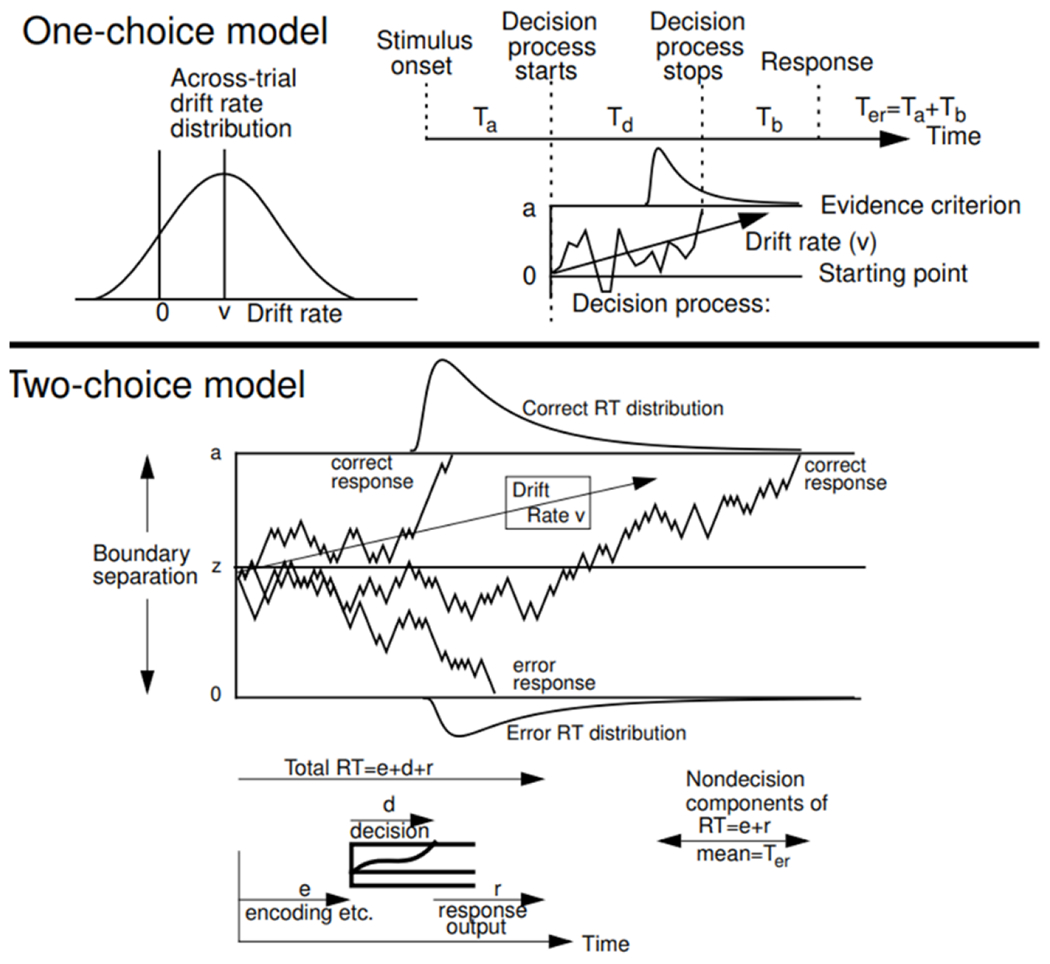
An illustration of the one-choice and two-choice diffusion models. For the one-choice model, evidence is accumulated at a drift rate v with normally distributed between-trial variability with standard deviation (SD) η, until it reaches a decision criterion a after time T_d. Additional processing time is represented by the nondecision time T_er, which includes stimulus encoding time T_a and response output time T_b. Nondecision time is assumed to be uniformly distributed across trials with range s_t. For the two-choice model, three simulated paths are shown with starting point z and boundary separation a. Drift rate is assumed to be distributed normally with mean v and SD η. Starting point is assumed to be distributed uniformly with mean z and range s_z. Nondecision time is composed of encoding processes, processes that turn the stimulus representation into a decision-related representation, and response output processes, and is assumed to be uniformly distributed with mean T_er and range s_t.

For the two-choice model, one path leads to a fast correct decision, one to a slow correct decision, and one to an error. Within-trial variability (noise) in the decision process gives rise to both right skewed RT distributions and also error responses when the process hits the wrong boundary by mistake. The rate at which evidence is accumulated toward one or the other choice is called drift rate (v). There is one decision criterion for the one-choice model and two for the two-choice model (Figure 1). For the one choice model, evidence begins at zero and the process terminates when the decision criterion set at a is reached. In the two-choice model, evidence begins at a starting point z and the process terminates when the process reaches one of two boundaries set at a or 0. For both models, the total time for a response to be made is the sum of the decision time and nondecision time. Nondecision time represents processes other than the decision process, which include stimulus encoding, motor planning, response output etc. These are collected into a single parameter with mean duration T_er (in the model analysis, these different components of nondecision time cannot be separated).

In order for the model to fit the relative speeds of correct and error RTs and the leading edges of RT distributions (see Ratcliff & McKoon, 2008), the components of processing are assumed to vary from trial to trial. Drift rate is assumed to be normally distributed with standard deviation (SD) η, nondecision time is assumed to be uniformly distributed with range s_t, and in the two-choice model, starting point is assumed to be uniformly distributed with range s_z. Also, in the two-choice model, a contaminant process representing random delays in processing was included in the modeling with the proportion of contaminants . There is a problem in identifiability in the one-choice model in that one of the model parameters needs to be fixed and then the others are identified (see Ratcliff & Van Dongen, 2011), therefore, the between-trial SD in drift rate parameter was fixed in the one-choice model.

The one-choice diffusion model was initially used in examining one of the principal tasks used to assess sleep deprivation, namely, the psychomotor vigilance task (PVT; e.g., Chavali, Riedy, & Van Dongen, 2017; Dinges & Kribbs, 1991; Dinges & Powell, 1985, Ratcliff & Van Dongen, 2011). Ratcliff and Strayer (2014) used the model to examine drivers’ vigilance by comparing the decision process in the PVT to the one-choice driving task. The results showed consistent individual differences in parameter values across tasks (i.e., significant positive correlations), suggesting that the two tasks tap into similar decision processes. Ratcliff and Strayer (2014) also used the one-choice diffusion model to examine the effect of distraction (i.e., talking on a cellphone) on the decision process during driving. The parameter values produced from fitting the model to data showed that longer mean RTs that occurred with distraction were mainly accounted by lower drift rates, (i.e., the quality of evidence driving the decision process) while the other model parameters were similar for the distracted and non-distracted conditions (see also Castro, Strayer, Matzke & Heathcote, 2019; Tillman, Strayer, Eidels & Heathcote, 2017). Ratcliff (2015) extended the diffusion model analysis to examine the relationship between the one-choice driving task and a two-choice brightness-discrimination driving task. The data were fit with the two-choice diffusion model and positive correlations were found for mean RTs, drift rates and nondecision time between the two driving tasks, suggesting that the two tasks and models were tapping into similar processes.

Diffusion models have been also used to examine the effect of aging on the decision process in a range of cognitive tasks (Ratcliff, Spieler & McKoon, 2000; Ratcliff, Thapar & McKoon, 2001; 2003; 2006; 2010; Ratcliff, Thapar, Gomez & McKoon, 2004; Starns & Ratcliff, 2010). In most of these studies, results showed that older adults have a longer nondecision time and a more conservative boundary separation than young adults. In many of these cases, older adults also had similar or slightly smaller drift rates compared to young adults, but in other tasks, differences in drift rates between age groups were quite large (e.g., associative recognition, Ratcliff, Thapar & McKoon, 2011; letter discrimination, Thapar, Ratcliff & McKoon, 2003). However, in the application to driving, the external constraints on the timing of behavior from traffic demands suggests that model components in driving tasks might behave differently relative to model components from the earlier laboratory studies. For example, (non-impaired) older drivers do not drive at half the speed or follow cars ahead of them at twice the distance of younger drivers. Furthermore, the older adults had been driving at least since their 20’s for over 40 years and so their driving skills were highly overlearned relative to the experience the they had with laboratory decision-making tasks.

To foreshadow our results, we found that older adults made more errors than young adults in the two-choice task, while differences in RT between age groups attenuated as the environment became more difficult. The models fitted the data well and showed consistent individual differences in parameter values across tasks. Results from the modeling analysis showed lower drift rates in older than young adults, which accounted for the decreased performance we found with age. However, it also appears that increased environmental difficulty, which produced lower drift rates for older adults, encouraged them to adjust the duration of the decision process by lowering their decision criteria to a greater extent than young adults.

Method

Transparency and openness

This research was performed in accordance with the Declaration of Helsinki and was approved by The Ohio State University Institutional Review Board (protocol #2003B0201). Informed consent was provided by all participants. The data that support the findings and the R code used to analyze this data are available. Fitting packages for the diffusion model are available from Voss & Voss (2007). The power of the current design to find significant effects was estimated using the simr package in R (Green & MacLeod, 2016). This study was not preregistered.

Participants

Thirty-one young adults (age range 19-29, 16 of them female) and forty-five older adults (age range 58-82, 30 of them female) were recruited through fliers posted on The Ohio State University campus and at Columbus-area senior recreation centers. The racial distribution across participants was not recorded. In exchange for participating in four experimental sessions, young adults and older adults were paid $12 and $15 per session, respectively. Prior to testing, all subjects completed the Mini-Mental State Examination (MMSE; Folstein, Folstein, & McHugh, 1975) to evaluate cognitive impairments; the Center for Epidemiological Studies-Depression Scale to evaluate mood (CES-D; Radloff, 1977); and the Vocabulary and Matrix Reasoning subtests of the Wechsler Adult Intelligence Scale – 3rd Edition to measure IQ (WAIS-III; Wechsler, 1997). Table 1 presents mean and SD values for these background measures (except for one older adult whose demographics and test scores are missing). The p-values in the table indicate significant differences between age groups for each characteristic. All subjects met test scores requirements for participation (26 or above on the MMSE and 6 or lower in the CES-D depression score). One young adult and sixteen older adults were excluded from the analysis (one young and six older adults were unable to perform the tasks, and ten older female adults suffered “simulator sickness” which made them nauseous and prevented them from performing the tasks). Participants in both age groups all had driving experience and were still regularly driving (the older adults had been driving since their 20’s).

Table 1.

Subject characteristics and p-values from t-tests comparisons between age-groups.

	Young		Older		p-value
	M	SD	M	SD
Age	22.56	2.53	68.45	13.79	<.001
Years of Education	14.38	2.24	15.46	2.77	.093
MMSE	29.3	0.75	28.21	1.50	.001
WAIS-III vocabulary (raw)	51.07	6.88	47.46	13.57	.215
WAIS-III vocabulary (scaled)	13.90	2.11	12.00	3.40	.015
WAIS-III matrix (raw)	21.23	3.23	14.54	5.84	<.001
WAIS-III matrix (scaled)	13.33	2.59	12.29	3.07	.164
WAIS-III IQ	120.70	10.30	111.86	15.08	.011
CES-D depression	1.73	1.78	1.63	2.36	.851
CES-D total	10.30	5.47	9.70	8.46	.756

Note. MMSE = Mini-Mental State Examination; WAIS-III = Wechsler Adult Intelligence Scale-3rd edition; CES-D = Center for Epidemiological Studies-Depression Scale.

Apparatus

The tasks were presented on a 15.6-inch Dell XPS L502SX laptop, with events sampled at a 16.67 ms rate. STISIM Drive software versions 2 and 3 were used to present the driving simulations in the two different landscapes. A Logitech Driving Force GT steering wheel with force feedback (http://www.logitech.com) and two pedals (accelerator and brake) were used to allow the participants to simulate driving.

Design & Materials

Three driving tasks were tested. Across tasks, participants were required to approach a “lead” car on each trial. When the driver was approximately 95 feet away from the lead car (for the one-choice task and two-choice clear task), the lead car wobbled left and right to indicate the trial’s onset. To simulate traffic demands, the driver was required to keep a constant distance from the lead car until the stimulus was displayed (about 65 mph in the one-choice and two-choice clear tasks and about 25 mph in the city task). The speed was controlled by the foot pedals).

In the one-choice task, the simulated driving environment included two lanes in a “clear” landscape. Driving was simulated during daytime, in an open space highway with gentle curves and only minor distractions on the side of the road. The simulator-display included speed and RPM meters and a rear-view mirror (see Figure 2, top-left panel). Both the driver’s car and the lead cars were placed in the right lane. When the brake lights of the lead car turned on, the driver was required to steer the car as quickly as possible into the left lane to avoid a collision with the decelerating car and to pass it. When the lead car receded to the rear (as could be seen in the rear-view mirror), the driver was required to steer the car back to the right lane and a new lead car appeared. The time interval between the trial’s onset and the brake lights’ display varied across trials from 2s to 10s with 2s-steps (Ratcliff, 2015).

Figure 2.

Example screen shots of driving views from the three driving tasks. The top-left panel shows the one-choice task when the brake lights of the lead car turned on. The top-right panel shows the two-choice clear task when a brightness-discrimination patch is displayed. The bottom panels show the two-choice city task with limited visibility with a brightness-discrimination patch (left panel) and a turn-message (right panel).

In the two-choice clear task, the simulated driving environment included three lanes in a clear landscape (Figure 2, top-right panel). Both the driver’s car and the lead car were placed in the middle lane. Instead of brake lights, a stimulus of a 64x64 array of black and white pixels (2.1x2.1 cm) was presented and the task was to drive into the right lane if the patch was bright (had more than 50% white pixels) and into the left lane if it was dark. The stimulus patch was displayed for 2 seconds between the two meters on the driver’s console and at the base of the lead car, between 0s and 8s (mean=4s) after the lead car wobbled to signal the trial’s onset. The probability of a pixel being white in the stimulus array was either .57, .53, .47, or .43 (the brightness conditions). To illustrate what is considered as a bright/dark patch, two example patches from each brightness condition were shown to the driver at the beginning of the task. Unlike the one-choice task, the driver was not asked to drive around the lead car, but to drive the car into the appropriate lane. After completing this manoeuvre, the drivers were instructed to drive the car back to the middle lane behind the lead car. The main purpose of the lead car in the two-choice clear driving task was to help the driver to maintain a fixed pace across trials.

The two-choice city task was similar to the two-choice clear task with the following exceptions: driving was simulated in a “city” landscape at night (i.e., restricted visibility ahead), in a single wide-lane (36 feet) urban road with two lines that indicated the road’s margins (i.e., ‘shoulders’; Figure 1, bottom panels). The road also included intersections and buildings on the side of the road. Unlike the clear version, the driver’s console included one speedometer and no rear-view mirror. To impose additional demands on the driving task, participants were required to make turns in the intersections in response to a displayed message (i.e., “turn right/left:” an example of this message is shown in Figure 1 bottom right). Either the turn message or brightness-discrimination patch appeared 90 feet before the centre of the next intersection, and the distance between intersections was 350 feet. After making a turn, the driver approached a new lead car. In cases in which the driver turned in an intersection without a preceding turn message, the following trial would present a patch without a lead car (90 feet before the intersection centre) and the experimenter would point out the error to the participant. The lead car pace was slower in the city version (25 mph) to allow driving in the city streets, including turns in the intersections. Finally, there was no wobble in the city version to indicate the trial’s onset.

Procedure

Participants completed four sessions that occurred, on average, once a week for young adults and twice a week for older adults. In the first three sessions, participants participated in all three tasks for approximately 15 minutes each (i.e., 45 minutes per session). The two-choice clear task had about 30% more observations per session than the other two tasks, so after three sessions a fourth was added in which the participants were tested on the one-choice task and the two-choice city task for 25 minutes each. Task order within each of the first three sessions was counterbalanced.

Participants were instructed they were about to perform a driving simulation task, in which they were required to drive in a simulated environment. In the one-choice and two-choice clear tasks, they were asked to approach a lead car on the road until it wobbled, and to maintain this distance until the stimulus was displayed. In the city landscape, there was no wobble, and if the driver’s car steered off the road and crashed into a building (e.g., when making a turn in the intersection), the driver was instructed to wait 15 seconds until the car was back on the road and then speed up to catch up to the next car (this occurred very infrequently). Finally, the driver was informed that using the brake pedal was unnecessary, as one could slow down by simply taking their foot off the gas pedal. To minimize potential dizziness or nausea during the driving tasks, we dimmed the lights in the testing room and encouraged participants to take breaks when needed.

Each task started with three practice trials. The number of experimental trials ended up differing between young and older adults and so we eliminated trials from some of the tasks to equate the average number of trials for young and older adults for each task. On average, the young and older adults had 173.0 and 172.6 trials in the one-choice task, 356.0 and 355.5 trials in the two-choice clear task, and 205.8 and 205.0 trials in the two-choice city task, respectively. For each trial, response times (in all tasks) and the corresponding response choices (in two-choice tasks) were recorded. A linear interpolation of the sideways velocity was used to estimate the time at which the car started to move sideways. The sideways velocity first increased and then became approximately constant for a short period of time as the car steered to the right or left. Linear interpolation from this relatively constant velocity provided an estimate of when the car began to turn, an estimate that was consistent across responses by the participant. In trials in which no action was recorded (e.g., the driver remained in the middle lane and did not swerve), the trial was not used in data analyses. Other details of the methods can be found in Ratcliff (2015).

Power analyses.

Because there is no agreed-upon analytic solution for calculating effect-sizes and power in mixed-effects models, we used the simr simulation package in R (Green & MacLeod, 2016) to estimate the power of the current design and statistical models to find significant effects between age groups (i.e., p<.05). Across a hundred simulations, we found 83% power to find an effect of age group on RT in the one-choice task; 36% power to find an effect of age group on RT in the two-choice tasks; and 96% power to find an effect of age group on accuracy in the two-choice tasks. Also, we found 90% and 88% power to find the anticipated interaction effect between age group and landscape on RT and accuracy, respectively; and 96% and 100% power to find a contrast effect (i.e., landscape×brightness interaction) on RT and accuracy, respectively.

For model parameters, Ratcliff and Childers (2015) performed a detailed analysis of the SDs in diffusion model parameters as a function of the number of observations from 80 to 1200 (dividing the experimental trials into different sized blocks). Results showed little change in model parameters within a session. So, for example, for 160 observations (Ratcliff & Childers, 2015, Table 1), the SD across participants in boundary separation was about 0.03, in nondecision time about 43 ms, and in drift rate, about 0.045 for difficult conditions. For 29 or 30 participants, standard errors (SEs) would then be divided by the square root of the sample size minus 1, which would give values of 0.006, 8ms, and 0.009 respectively. This means that for two groups, 2 SE (combined) differences (which are detectable based on other published experiments) would be 0.009, 11ms, and 0.012. These are smaller than differences we obtained in this experiment.

Results

Behavioral results

We analyzed the data from the one-choice task and the two-choice tasks separately, because the two tasks have different dependent variables (i.e., only RT in the one-choice task, but RTs for correct and error responses and probability correct in the two-choice task). For the one-choice data, we used a linear mixed-effects model with RTs as the dependent variable, age group (i.e., young vs. older) as a fixed factor and participants as a random intercept effect. For the two-choice data, we used a similar model but with landscape (i.e., clear vs. city), age group and brightness as fixed factors. To simplify the statistical analysis, we collapsed the four conditions of brightness into darker (.43 and .47) and brighter (.53 and .57) conditions. All the statistical tests were two-sided. The mean RT values for the collapsed brightness conditions between age-groups and landscapes are presented in Figure 3A. Low RT cutoffs were set to 150 ms in the one-choice task and 400 ms in the two-choice tasks, and upper RT cutoffs were set to 4000 ms across tasks. On average, 0.6%, 1.5% and 0.4% of the young-adult responses and 4.1%, 4.3% and 1.3% of the older-adult responses were excluded from the one-choice, two-choice clear and two-choice city tasks, respectively.

Figure 3.

The mean RTs for age groups and landscape condition in the two-choice driving tasks (panel A), and the proportions of correct responses for the same conditions (panel B). Error bars correspond to the within-subjects standard error¹. Correct RTs for “bright” responses to bright stimuli are collapsed with correct “dark” responses to dark stimuli. The same combinations are used for probability correct.

A main effect for age group in the one-choice task (χ²(1)=8.2, p=.004) showed that mean RT values (in milliseconds; SD represents the standard deviation of the mean RT values across participants) were significantly longer for older (M=711, SD=129) than young adults (M=639 SD=69). In the two-choice driving tasks (Figure 3A), we found null differences in RTs between age groups across tasks (χ²(1)=2.0, p=.160), and a main effect for landscape across age groups (χ²(1)= 558.8, p<.001) - showing that on average, RTs were longer under the more demanding city landscape (M_clear=986, SD=148; M_city=1063, SD=182). Importantly, we found a significant interaction between age group and landscape (χ²(1)=11.1, p<.001), which showed that differences in RTs between age groups attenuated as the environment became more difficult. Thus, the age difference in RT was larger in the easier landscape, but in neither condition did the age difference reach significance. In particular, the difference in mean RTs between young and older adults was marginally significant in the two-choice clear task (M_young=954, SD=130 vs. M_older=1018, SD=160; χ²(1)=3.0, p=.084), and non-significant in the two-choice city task (M_young=1043, SD=188 vs. M_older=1083, SD=176; χ²(1)=0.8, p=.385). This is likely because older adults cannot slow down as much as they do in more standard laboratory tasks because driving imposes external constraints from traffic-demands. Finally, we found a main effect for brightness (χ²(1)=36.9, p<.001) and an interaction effect between landscape and brightness (χ²(1)=47.7, p<.001). The interaction shows a contrast effect, in which participants responded faster to darker than brighter patches in the bright clear landscape (M_brighter=1004, SD=160 vs. M_darker=967, SD=143; χ²(1)=80.8, p<.001), while small (and nonsignificant) differences in the opposite direction were obtained in the dark city landscape (M_brighter=1059, SD=183 vs. M_darker=1066, SD=190; χ²(1)=2.5, p=.113).

To test the effect of age on accuracy as a function of brightness and landscape, we tested a probit mixed-effects model with the proportion of correct responses (p[correct]) as the dependent variable (Figure 3B). We found a main effect for age group (χ²(1)=11.2, p<.001), suggesting that on average, young adults (M=.82, SD=.07) were more accurate than older adults (M=.76, SD=.07) across the two-choice driving tasks. Moreover, a main effect for landscape (χ²(1)=243.6, p<.001) indicated that p(correct) decreased as the environment became more difficult (M_clear=.83, SD=.08 vs. M_city=.76, SD=.09). We also found a main effect for brightness (χ²(1)=73.6, p<.001), but more importantly, a two-way interaction between landscape and brightness (χ²(1)=232.6, p<.001) showed that p(correct) was higher for darker than brighter patches in the two-choice clear task (M_Brighter=.78, SD=.10 vs. M_Darker=.87, SD=.12; χ²(1)=265.6, p<.001), while the opposite trend was obtained in the two-choice city task (M_Brighter=.78, SD=.13 vs. M_Darker=.73 SD=18; χ²(1)=38.0, p<.001). This pattern of results shows that the simulated landscape (i.e., clear or city) produced a contrast effect on the perception of brightness (as for mean RT), so that a bright patch on a dark background was perceived as brighter than a bright patch on a bright background (see Figure 1).

Finally, a two-way interaction effect between age group and landscape (χ²(1)=7.0, p=.008) along with a three-way interaction among all factors (χ²(1)=46.9, p<.001) suggested that environment difficulty reduced accuracy to a greater extent for older than younger adults. In particular, older adults performed worse in the city landscape than the clear landscape across brightness conditions, while the opposite trend was obtained for young adults when the stimulus was brighter. This is because the contrast between the brighter stimulus and the darker city landscape (i.e., the contrast effect) made the discrimination task easier, despite the difficulties imposed by the city landscape. However, for older adults the contrast effect only attenuated the decrease in accuracy with environment difficulty, illustrating the greater challenges older adults might experience in diving attention between the decision task and driving in the demanding city landscape (Figure 3B).

Model-based results

Overall, four parameters were estimated from fitting the one-choice model: v, T_er, S_t, and a (the SD of within trial variability was fixed to .1 and η was fixed to .2). In the two-choice model, eleven parameters were estimated, including four drift rates, one for each brightness condition (v₁-v₄) An overall value of drift rate (V) was computed by (v₁+v₂−v₃−v₄)/4. The models were fitted to the data from the one- and two-choice driving tasks for each participant separately to allow individual differences to be examined. Correlations between the drift rate, boundary setting, and nondecision time parameter values across tasks were examined to determine whether it is plausible that the tasks tapped into a common decision mechanism. The goodness-of-fit of each model was estimated from χ² values from the observed and the predicted quantile data. See section A1 in the Appendix for more details about the fitting method.

The quantile RTs averaged over participants and the models’ predictions averaged over participants are displayed in Figure 4, showing a good fit to data. The mean parameter values and estimates for the goodness-of-fit at the group level (mean χ² values) and at the individual level (the number of participants with χ² less than the critical value, ${\chi }_c^2$ ) are presented in Tables 2 and 3. The critical χ² values were 23.7 with 14 degrees of freedom for the one-choice model and 47.4 with 33 degrees of freedom for the two-choice model. Across tasks and age groups, the mean chi-square values were below the critical values. At the individual level, the majority of participants across age groups and tasks had χ² values that were below the respective critical value (see Table 2).

Figure 4.

Fits of the models to data. A) Cumulative RT distributions averaged over participants for young and older adults in the one-choice driving task. The ‘o’s are the data and the ‘x’s are the model predictions. B) Quantile-probability functions averaged over participants for young and older adults in the two-choice clear and city driving tasks. The values on the x-axis represent the proportion of responses for the brightness conditions. In the top plots, the brightness conditions from right to left are .43, .47, .53, .57 white pixels, and for the bottom plots the order is reversed. The quantile response times are marked on the y-axis by different colors. In order from the bottom to the top, the quantiles are .1, .3, .5, .7, and .9 (colored in black, red, green, blue and cyan, respectively). In both panels, x’s represent the behavioral data and lines and o’s represent the theoretical fits of the diffusion models. In some of the conditions representing errors on the left sides of the plots, only a median (green x’s) is plotted when there are less than 5 observations for some of the participants, and nothing is plotted when some have no errors in that condition.

Table 2.

Mean parameter values across participants from the one-choice and two-choice diffusion models.

Task-version	Age	a	z	T er	η	sz	st	po	χ2	N(<${\chi }_c^2$¿
One-choice Clear	Young	0.220		0.352	0.200		0.205		12.2	29/30
	Older	0.200		0.339	0.200		0.238		8.6	27/29
Two-choice Clear	Young	0.137	0.071	0.701	0.167	0.041	0.368	0.002	33.4	28/30
	Older	0.145	0.070	0.714	0.149	0.044	0.479	0.002	43.3	19/29
Two-choice City	Young	0.129	0.068	0.804	0.170	0.035	0.309	0.005	31.6	29/30
	Older	0.122	0.058	0.845	0.135	0.057	0.410	0.001	41.9	19/29

Note: a represents the decision boundary separation; z represents the starting point; T_er represents nondecision time; η represents standard deviation in drift rate across trials; s_z represents range of the distribution of starting points (z); s_t represents range of the distribution of nondecision times; p_o represents proportion of contaminants; χ² represents the average goodness-of-fit (group level); and N(< ${\chi }_c^2$]¿ represents the number of participants with χ² value below the critical value (out of N=30 for young adults and N=29 for older adults). The critical χ² values were 23.7 with 14 degrees of freedom for the one-choice model and 47.4 with 33 degrees of freedom for the two-choice model.

Table 3.

Mean drift rate values across participants from the one-choice and two-choice diffusion models

Task-version	Age	v1	v2	v3	v4	V
One-choice Clear	Young					0.866
	Older					0.691
Two-choice Clear	Young	0.296	0.117	−0.212	−0.383	0.252
	Older	0.244	0.083	−0.143	−0.325	0.199
Two-choice City	Young	0.323	0.139	−0.128	−0.353	0.236
	Older	0.245	0.084	−0.067	−0.198	0.148

Note: v₁, v₂ are for bright stimuli (.57 and .53 white pixels respectively) and v₃, v₄ are for dark stimuli (.47 and .43 white pixels respectively); V represents the overall drift rate. For the two-choice driving task it is (v₁+v₂−v₃−v₄)/4.

Parameter values

We used independent sample t-tests to examine the differences between age groups in parameter values (Table 2 and 3) in the one-choice driving task, and a repeated measure MANOVA test for differences in parameters values between age groups and landscape conditions in the two-choice task. The mean values of the main parameters (a, Ter and V) among age groups and tasks are presented in Figure 5, and the t and F statistics from the respective tests are presented in Table 4. Findings show that across tasks, average drift rates were significantly lower for older than young adults, which largely accounts for longer RTs (one-choice task) and lower accuracy (two-choice tasks) found in the older group. Drift rates were also significantly lower in the city condition than the clear condition across age groups, accounting for the decreasing accuracy and longer RTs found in the more difficult city environment. We also found lower boundary separation in the city than clear condition, and an interaction effect for boundary separation between landscape and age group. This interaction showed that differences in boundary separation between the clear and city landscapes were larger for older than young adults. In addition, we found a significantly longer nondecision time in the city condition than the clear condition, a lower across trial range in nondecision time (s_t) in the city condition than the clear condition, and a lower value of s_t in older adults than young adults. Finally, there was no difference in the relative bias in starting point (i.e., z/a) between the city and clear conditions nor an interaction with age group.

Figure 5.

The mean values of boundary separation, nondecision time and drift rate among age groups and tasks. Error bars correspond to standard errors.

Table 4.

The t statistics with 57 degrees of freedom from the independent sample t-tests for differences in parameter values among age-groups in the one-choice task; and the F statistics with the [1,58] degrees of freedom from the two-way repeated measures MANOVA test for differences in the parameters’ values among landscape and age-groups

Task	Factors	a	z	T er	η	sz	st	V	p0	z/a
One-choice	Age group	1.87	-	1.19	-	-	−1.47	3.00	-	-
Two-choice	Age group	0.00	1.69	1.22	2.80	3.0	13.91	11.15	1.97	3.54
	Landscape	24.07	8.13	59.39	0.10	0.20	10.82	7.74	0.62	0.36
	Landscape × Age group	5.46	3.79	0.90	0.27	1.50	0.06	2.06	1.75	0.74

Note: Significant effects are marked in bold (p<.05).

Together, these results show the challenges that older adults might have experienced in dividing attention between the decision tasks and driving while following traffic demands. Lower drift rates accounted for the decreasing accuracy and longer RTs we found in older adults and in the more difficult city environment. Importantly, low drift rates would produce long RTs that might exceed the constraints of traffic demands. Consequently, results showed that older adults were induced to lower boundary separation to a greater degree than young adults in order to compensate for a slower decision process. In other words, when the environment difficulty increased (i.e., two-choice clear vs. city), greater adjustments were required to speed the decision process and larger differences in boundary separation between young and older adults emerged. Finally, longer nondecision time in the city than clear landscape accounted for additional delays in response time as the task became more difficult.

The contrast effect found in the behavioral data between the simulated landscape and the brightness level of the patch was also captured in the model by a drift rate bias. A repeated measures analysis for differences in drift rates revealed a significant interaction between landscape and brightness (collapsed across age groups and the two levels of brighter and darker patches; F[1,58]=7.5, p=.008); showing that the absolute drift rate value in the clear condition was higher for darker than brighter stimuli (M_brighter=0.19, SD=.11 vs. M_darker=−0.27, SD=.13), while the opposite trend was obtained in the city condition (M_brighter=0.20, SD=.11 vs. M_darker=−.19, SD=.17).

Individual differences

If the one- and two-choice models tapped on a common decision mechanism across driving tasks, then there should be positive correlations between the corresponding parameters for the two models. The Pearson correlation coefficients for mean RTs, p(correct) and the mean parameter values between three comparison pairs of the one- and two-choice driving tasks for each age group are presented in Table 5. For more detailed correlation matrix, see Figure A1 in the Appendix (note that neither age nor the MMSE scores correlate with any diffusion model parameters). There are numerous correlations that can be tested, but we decided to focus on the ones that were large and/or of theoretical interest. Between the two-choice driving tasks, we found positive and significant correlations for mean RTs, p(correct), drift rate, nondecision time and boundary separation, suggesting that the two-choice diffusion model successfully captured common mechanisms across tasks. Moreover, we found positive correlations for nondecision time between the one- and two-choice tasks across age groups, showing that encoding and response requirements account for a significant portion of individual differences in RTs. In contrast to findings in Ratcliff (2015), we did not find significant correlations for mean RTs and drift rates between the one- and two-choice tasks, except for a positive and significant correlation for drift rates between the one-choice task and the two-choice clear task in older adults, which shows consistency between the two tasks. Note that the number of observations in the one-choice task in the current study was almost half of the number of observations in the one-choice task in Ratcliff (2015), which reduced the statistical power for the correlation analysis. Moreover, although the mean RTs were not significantly correlated between the one- and two-choice tasks, all correlation values were moderate and positive, which is unlikely if all the true correlations were zero. This is because the probability of getting all four values above zero is .0625 (0.5 raised to the fourth power), and the probability of obtaining four values above .18 (the lowest of the four correlations shown in Table 5) is 8.9×10⁻⁴. This is also true for the nonsignificant but moderate correlations we found for nondecision time and drift rate for older adults. Consequently, we argue that the diffusion model framework was able to identify common features of the decision process across tasks.

Table 5.

The Pearson correlation statistics for mean RTs, p(correct) and the parameter values among pairs of tasks for the different age groups

Pairs of driving tasks	Age group	Mean RTs	T er	V	p(correct)	a
Two-choice clear and city	Young	.87	.58	.51	.53	.63
	Older	.78	.38	.55	.67	.62
One-choice and Two-choice clear	Young	.18	.44	.02
	Older	.32	.49	.42
One-choice and Two-choice city	Young	.28	.59	.11
	Older	.23	.64	.25

Note: Significant correlations are marked in bold (p<.05).

Discussion

This experiment addresses two issues in driving behavior using a diffusion model analysis of the components of decision making to explain response time and the accuracy rates in simulated driving tasks. The issues are: how does the decision-making behavior of older versus young adults compare in a simulated driving task and what happens if the driving task becomes more difficult due to higher demands on the driving, decision, and response processes? As noted in the introduction, driving in older adults is of great concern and here we present the first study that uses one-choice and two-choice driving tasks and models that begin to examine the components of decision processes while driving in older relative to young adults under increasing environmental difficulty. The one-choice driving task provided a way of examining a single response to a single event during driving, and the two-choice task provided measures of both RT and accuracy when the decision involved one of two possible driving responses.

Results from the two-choice tasks showed that older drivers were more prone to make mistakes in the decision task than young drivers, and this trend was larger with higher demands imposed by the (city versus the clear) environment. Differences in RT between older and young participants were not as large as in similar aging studies that tested cognitive tasks in the laboratory (e.g., Ratcliff et al., 2000; Ratcliff et al. 2001; 2003; 2006; Starns & Ratcliff, 2010). We argue that this is because response time on the road is mostly determined by traffic demands, i.e., driving behavior is usually aligned with the behavior of other drivers on the road in order to maintain a cohesive traffic stream. Hence, older drivers (that are not seriously impaired) have to slow down and speed up with other drivers and could not, for example, take twice the time to perform such tasks. This forces older adults to conform to traffic demands, stressing speed at the expense of accuracy. Consistent with this notion, the increase in RT with environment difficulty (i.e., clear vs. city) was larger for young adults, while the decrease in accuracy was larger for older adults. Furthermore, our older drivers were extremely experienced, and most had been driving for over 40 years, hence the task was highly overlearned. In contrast, in laboratory studies, the tasks and response requirements are not overlearned leading to greater differences between older and young adults.

The behavioral results were well fit by the diffusion model with straightforward interpretations of the effects of age and environment difficulty on model components. Furthermore, many of the model parameters were correlated across tasks. This finding is important because the tasks differ in the response requirements and in the dependent variables (the one-choice task has only RT whereas the two-choice task has correct and error RTs and accuracy). This means that the diffusion model framework successfully identified common processes across the two tasks which supports the conclusions drawn from the parameter-value analysis.

A comparison of parameter values between age groups and tasks showed that differences in the decision-making tasks between older and young drivers were mostly explained by lower drift rates for older than young adults, which accounted for lower accuracy rates found in the older group. This is different from previous results that showed similar drift rates across age groups in the brightness discrimination task (e.g., Ratcliff et al., 2003). One plausible explanation for this is that older adults often show difficulties in dividing attention between tasks (e.g., Ging-Jehli & Ratcliff, 2020; Kramer & Kray, 2006; Parasuraman & Nestor, 1991; Verhaeghen & Cerella, 2002). Consequently, they might experience difficulties in dividing attention between the decision task and driving, especially when the demands imposed by the environment are high, thus reducing the rate of evidence accumulation (i.e., a result similar to the effect of using a cell-phone during driving in Ratcliff & Strayer, 2014). Another possibility is that the implicit stress of speed, imposed by environment difficulty and traffic demands, might have been responsible for the reduced drift rates. This is because motor processes are often slower in older age (Falkenstein, Yordanova & Kolev, 2006; Gaspar et al., 2013; Ward, 2006), and so to compensate, stimulus encoding might be abbreviated in the effort to speed nondecision processes and make responses consistent with traffic demands, resulting in lower drift rates (see Starns, Ratcliff, and McKoon, 2012 for results that demonstrate this reduction in drift rate with high speed-stress). A third possibility is that the brightness patch in the two-choice driving tasks was smaller than in previous non-driving experiments, hence, reducing acuity and so possibly reducing the quality of the encoded stimulus.

We also found that nondecision time was longer in the city landscape than the clear landscape, probably because the pace of the lead car was slower in city (25mph) than clear (65mph) conditions, allowing for slower responses in the former. However, unlike common findings from similar aging studies (e.g., Ratcliff et al., 2003; 2006), we did not find evidence for slower nondecision processes in older than young adults. This is because RTs had an upper limit set by traffic demands, resulting in small or no differences in RTs between age groups and consequently, null differences in nondecision time as well (and the older adults were highly practiced at driving). Consistent with this observation, we found lower boundary separation for older than young adults as the environmental difficulty increased. That is, the rate of evidence accumulation in older drivers was lower when the demands from the environment increased (e.g., clear vs. city), which induced them to make adjustments to the duration of the decision process in order to fit traffic demands. This was achieved by lowering the decision criteria to a greater degree than young drivers, leading to slightly more errors. Note that adjusting boundary separation in response to a speed-stress manipulation is a common effect found in cognitive tasks in the laboratory (Ratcliff et al., 2001, 2003, 2004; Thapar et al., 2003), therefore, it is often attributed to be under the control of the decision maker. We argue that older adults made similar adjustments to the decision criteria in response to an implicit speed-stress imposed by environment difficulty and traffic demands (see also Vanunu & Ratcliff, 2022).

Nevertheless, one advantage of a model-based analysis is to allow us to make predictions for what would happen if one or more model components changed. Older adults reduced their boundary separation from the clear to the city landscape to compensate, we assume, for increased difficulty. To illustrate the effect of this compensation, we generated predicted values of accuracy and mean correct RT (averaged over the four brightness conditions) for the parameter values for the city landscape for older adults from Table 2 (with boundary separation 0.122). We then asked what would have happened if boundary separation was set at the value for the clear landscape (0.145) with all other parameters held at the values for the city landscape. If boundary separation increased from 0.122 to 0.145, accuracy would increase slightly by 1% (from .725 to .735) and mean correct RT would increase by 80 ms (from 1089 to 1167 ms). For comparison, using the parameters for the clear environment, accuracy was .819 and mean correct RT was 1038 ms. Thus, reducing boundary separation instead of leaving it at the value used for the clear landscape compensated for 78 ms of the 129 ms increase in mean correct RT relative to the clear environment that would have occurred if boundary separation was not changed (at the cost of about 1% in accuracy). Consequently, we conclude that lower drift rates (in response to difficulties in switching attention or to speed-stress by traffic demands) were the primary factor for the reduced accuracy found in older adults.

It is important to note that across studies we measured the behavior in decision-tasks that require a driving response while operating a PC-based driving simulator, rather than measuring real driving behavior on a road (e.g., lane-keeping, speeding and slowing in response to traffic demands, etc.). However, drivers make behavioral responses to factors external to the mechanics of driving all the time and our modeling addresses this behavior. Recent studies have extended the use of the diffusion model framework to capture the underlying mechanism of various driving actions such as making a left turn across traffic in the opposite direction (Zgonnikov, Abbink & Markkula, 2020); steering and gear shift paddle behavior in response to a decelerating car (Markulla, 2014; Markkula, Engström, Lodin, Bärgman, & Victor, 2016; Xue, Markkula, Yan, Merat, 2018); and estimating the time to collision (Daneshi, Azarnoush & Towhidkhah, 2020; Daneshi, Azarnoush, Towhidkhah, Gohari & Ghazizadeh, 2019). For instance, Xue et al. (2018) proposed a model of driving behavior to explain the response of drivers to a decelerating lead car. The model assumes a diffusion process of evidence accumulation towards a threshold - collected from multiple cues such as visual looming metrics (i.e., the angular expansion rate of a lead car on the driver’s retina) and braking lights. Findings from a model-comparison analysis revealed that the diffusion model produced a better fit to data than a common earlier model of driving behavior, which considered visual looming metrics alone (e.g., Maddox & Kiefer, 2012). Such studies along with the results presented here show the utility of applying diffusion model analyses to driving tasks.

Conclusions

Response time in real-world driving is determined to a large degree by traffic demands and so if some components of decision-making processes slow with age, drivers must try to compensate by speeding up other components. In our experiments, we found that in a more difficult driving environment, even though older adults were more likely to make more errors than young adults in the decision task, differences in RTs were relatively small between age groups. A diffusion model analyses showed a good fit to data and consistent individual differences in parameter values across tasks, suggesting common components of decision processes during the driving tasks. Results from the model-based analysis suggested that difficulties in dividing attention between driving and performing the decision tasks for older adults might have interfered with evidence accumulation, explaining the reduced accuracy and slower responses found in this group. Results also showed that to compensate for lower evidence accumulation as the driving task environment became more difficult, older adults reduced the duration of the decision process by reducing decision boundary separation. This boundary-decrease did not affect accuracy by much (1%), which shows that this type of adjustment is relatively “safe”. However, it is possible that older drivers made additional adjustments to stimulus encoding in the effort to speed nondecision processes, producing lower-quality evidence (lower drift rates) and hence lower accuracy.

These results show subtle patterns of behavior and compensatory behavior in our driving tasks. Generally, the data from these tasks are well fit by the diffusion models, provide interpretable effects within each task and interpretable difference between tasks. Thus, these results validate the use of the models and experimental methods in understanding the effects of age on driving. We argue that it is important to map out how the components of decision-making processes in driving tasks change with traffic and driving environment demand, task difficulty, and all kinds of other factors such as distraction and attention. Identifying how these factors change with age and driving conditions will inform policy makers or engineers in designing assessments and driving aids that can be used to improve safety for older drivers. Specifically, if information about how a specific device or driving aid affects performance in driving, it could be added to driving tasks like those studied here, in easy and difficult driving environments. The diffusion model analyses could be used to see the effects on caution and evidence used in the decision process. What our analyses provide is a method for examining decision-making processes in driving.

Public Significance Statement:

While driving in a screen-based simulator, older and younger adults performed three decision-making tasks. Findings showed that older adults were slower to respond and made more errors than young adults. A diffusion modeling analysis identified which component of the decision process change with age, showing lower rates of evidence accumulation and lower decision criterions for older than young drivers. This information can inform design of driver aids, warning systems, driver assessment and training for older adults.

With an increase in life expectancies, the number of licensed elderly drivers has significantly increased in the past few decades. According to the U.S. Department of Health and Human Services, between 2001 and 2018 there was a 60% increase in the number of older drivers on the road (Centres for Disease Control and Prevention, n.d.). Although older drivers do not necessarily experience more car accidents than young drivers, they are more likely to suffer fatalities due to increased fragility (Li, Braver & Chen, 2003). In fact, twenty older drivers are killed and seven hundred are injured every day due to traffic accidents (Centres for Disease Control and Prevention, n.d.). Consequently, a substantial amount of research has been performed to identify the effect of aging on various perceptual and cognitive functions that are components of the skill of driving.

Appendix

A1. Fitting method

The decision in response to the stimulus in each case involved changing direction by either driving around the car ahead or driving to the side and back. For each trial, the response was recorded from the change in direction initiated by moving the steering wheel. For the two-choice model, we used the standard explicit solution to fit the model to data (see Ratcliff & Tuerlinckx, 2002). However, although there is an explicit solution for the distribution of RTs for a positive drift rate in the one-choice model (the Wald or inverse Gaussian distribution), there is no explicit solution for a RT distribution generated by a negative drift rate (produced from the left tail of the between-trial distribution of drift rate; see Figure 1). Therefore, we fitted the one-choice model by simulating the process, using a random walk approximation to the diffusion process as in Ratcliff and Van Dongen (2011). Each simulated condition used 20,000 iterations with a 0.5-ms step size (Tuerlinckx, Maris, Ratcliff & De Boeck, 2001). We set the maximum response time in the simulation to 3000 ms for young adults and 6000 ms for older adults, and any RT that exceeded this boundary was set to this maximum value (this occurred 0.2 and 1.1 % of the time for young and older adults respectively). We used 5 quantiles of the two RT distributions for correct and error responses (i.e., .1, .3, .5, .7 and .9) to fit the two-choice model. For the one-choice model, there is only one RT distribution, which makes it important to use as much distributional information as possible. Therefore, we used 19 quantiles of the RT distribution to fit the one-choice model, with a step of .05 between quantiles (i.e., .05, .1, .15, etc.). Importantly, we grouped the first and second quantiles in the one-choice model to produce more stable estimates of the leading edge of the RT distribution (by minimizing the effects of a few anticipations that produced extremely short RTs, see Ratcliff & Strayer, 2014). The fit for an individual participant took about 20 seconds on a 64 core workstation.

We optimized the parameters of the model by using a simplex minimization routine to minimize the chi-square value - calculated as Σ(O—E)²/E. The observed values (O) were calculated by multiplying the total number of observations by the proportions of responses between the data quantiles (e.g., .05 in the one-choice model). The expected values (E) were calculated by multiplying the total number of observations with the proportion of responses in the predicted RT distribution that laid between the data quantiles (predicted from the explicit solution for the two-choice model or the simulation routine for the one-choice model). Contributions were computed separately for correct responses and error responses. The simplex minimization routine was restarted 18 times with a wide simplex round the parameters estimated from the prior fit (though usually only 4 or 5 restarts were needed). Because of the issue of parameter identifiability in the one-choice model, we fixed η to .2 when fitting this model to data, as we felt it is the most appropriate value for the current data set. In both models, we fixed the within trial SD to .1.

Both models were fitted to each individual participant separately to allow individual difference analyses. To estimate the goodness-of-fit of the models, the average chi-square value across participants in each age group and driving task was compared to a respective critical value ( ${\chi }_c^2$¿ . To represent the goodness-of-fit at the individual level, we counted the number of participants in each group and task with χ² smaller than the critical value (i.e., N[< ${\chi }_c^2$ ]). Finally, we analyzed the relationships and differences between parameter values across age groups and tasks. We assumed that significant correlations among parameter values would serve as evidence for a common decision process across tasks, while significant differences among the mean parameter values would show the influence of aging and environment difficulty on the decision process in driving.

A2. Scatter plots and correlation matrices

Figure A1.

Scatter plots, histograms, and correlations for boundary separation, nondecision time and drift rate in each age group and task, and for age and MMSE scores.

References

- Burns PC, Trbovich PL, McCurdie T, & Harbluk JL (2005, September). Measuring distraction: Task duration and the lane-change test (LCT). In Proceedings of the Human Factors and Ergonomics Society Annual Meeting (Vol. 49, No. 22, pp. 1980–1983). Sage CA: Los Angeles, CA: SAGE Publications. [Google Scholar]
- Castro SC, Strayer DL, Matzke D, & Heathcote A (2019). Cognitive workload measurement and modeling under divided attention. Journal of Experimental Psychology: Human Perception and Performance, 45(6), 826–839. [DOI] [PubMed] [Google Scholar]
- Centers for Disease Control and Prevention (n.d.). Older Adult Drivers. https://www.cdc.gov/transportationsafety/older_adult_drivers/index.html
- Chavali VP, Riedy SM, & Van Dongen H (2017). Signal-to-noise ratio in PVT performance as a cognitive measure of the effect of sleep deprivation on the fidelity of information processing. Sleep, 40(3). [DOI] [PMC free article] [PubMed] [Google Scholar]
- Cooper JM, & Strayer DL (2008). Effects of simulator practice and real-world experience on cell-phone—related driver distraction. Human Factors, 50(6), 893–902. [DOI] [PubMed] [Google Scholar]
- Cousineau D (2005). Confidence intervals in within-subject designs: A simpler solution to Loftus and Masson’s method. Tutorials in quantitative methods for psychology, 1(1), 42–45. [Google Scholar]
- Daneshi A, Azarnoush H, & Towhidkhah F (2020). A one-boundary drift-diffusion model for time to collision estimation in a simple driving task. Journal of Cognitive Psychology, 32(1), 67–81. [Google Scholar]
- Daneshi A, Azarnoush H, Towhidkhah F, Gohari A, & Ghazizadeh A (2019). Drift-diffusion explains response variability and capacity for tracking objects. Scientific reports, 9(1), 1–15. [DOI] [PMC free article] [PubMed] [Google Scholar]
- Dinges DF & Powell JW (1985) Microcomputer analyses of performance on a portable, simple visual RT task during sustained operations. Behavior Research Methods Instruments and Computers, 17, 652–655. [Google Scholar]
- Dinges DF & Kribbs NB (1991). Sleep, Sleepiness and Performance (Monk TH, Ed.). Wiley, Chichester, pp 97–128. [Google Scholar]
- Engström J, Markkula G (2007). Effects of visual and cognitive distraction on lane change test performance. In Proceedings of the Third International Driving Symposium on Human Factors in Driver Assessment, Training and Vehicle Design (pp. 199–205). Iowa City: University of Iowa. [Google Scholar]
- Falkenstein M, Yordanova J, & Kolev V (2006). Effects of aging on slowing of motor-response generation. International Journal of Psychophysiology, 59(1), 22–29. [DOI] [PubMed] [Google Scholar]
- Folstein MF, Folstein SE, & McHugh PR (1975). “Mini-mental state”: a practical method for grading the cognitive state of patients for the clinician. Journal of psychiatric research, 12(3), 189–198. [DOI] [PubMed] [Google Scholar]
- Gaspar JG, Neider MB, & Kramer AF (2013). Falls risk and simulated driving performance in older adults. Journal of Aging Research, 2013. Article ID 356948. [DOI] [PMC free article] [PubMed] [Google Scholar]
- Ging-Jehli NR, & Ratcliff R (2020). Effects of aging in a task-switch paradigm with the diffusion decision model. Psychology and Aging, 35(6), 850–865. [DOI] [PMC free article] [PubMed] [Google Scholar]
- Green P, & MacLeod CJ (2016). SIMR: an R package for power analysis of generalized linear mixed models by simulation. Methods in Ecology and Evolution, 7(4), 493–498. [Google Scholar]
- Hoffman L, McDowd JM, Atchley P, & Dubinsky R (2005). The role of visual attention in predicting driving impairment in older adults. Psychology and Aging, 20(4), 610–622. [DOI] [PubMed] [Google Scholar]
- ISO/DIS 26022 (2010). Road Vehicles - Ergonomic Aspects of Transport Information and Control Systems - Simulated Lane Change Test to Assess In-vehicle Secondary Task Demand. Geneva, Switzerland: ISO. [Google Scholar]
- Kramer AF, & Kray J (2006). Aging and Attention. In Bialystok E & Craik FIM (Eds.), Lifespan cognition: Mechanisms of change (p. 57–69). Oxford University Press. [Google Scholar]
- Li G, Braver ER, & Chen LH (2003). Fragility versus excessive crash involvement as determinants of high death rates per vehicle-mile of travel among older drivers. Accident Analysis & Prevention, 35(2), 227–235. [DOI] [PubMed] [Google Scholar]
- Madden DJ (2007). Aging and visual attention. Current Directions in Psychological Science, 16(2), 70–74. [DOI] [PMC free article] [PubMed] [Google Scholar]
- Maddox ME, & Kiefer A (2012, September). Looming threshold limits and their use in forensic practice. In Proceedings of the Human Factors and Ergonomics Society Annual Meeting (Vol. 56, No. 1, pp. 700–704). Los Angeles, CA: SAGE Publications. [Google Scholar]
- Markkula G (2014, September). Modeling driver control behavior in both routine and near-accident driving. In Proceedings of the human factors and ergonomics society annual meeting (Vol. 58, No. 1, pp. 879–883). Los Angeles, CA: SAGE Publications. [Google Scholar]
- Markkula G, Engström J, Lodin J, Bärgman J, & Victor T (2016). A farewell to brake reaction times? Kinematics-dependent brake response in naturalistic rear-end emergencies. Accident Analysis & Prevention, 95, 209–226. [DOI] [PubMed] [Google Scholar]
- Mattes S (2003). The lane-change-task as a tool for driver distraction evaluation. Quality of Work and Products in Enterprises of the Future, 57, 60. [Google Scholar]
- Parasuraman R, & Nestor PG (1991). Attention and driving skills in aging and Alzheimer’s disease. Human Factors, 33(5), 539–557. [DOI] [PubMed] [Google Scholar]
- Perryman KM, & Fitten LJ (1996). Effects of normal aging on the performance of motor-vehicle operational skills. Journal of Geriatric Psychiatry and Neurology, 9(3), 136–141. [DOI] [PubMed] [Google Scholar]
- Petzoldt T, Brüggemann S, & Krems JF (2014). Learning effects in the lane change task (LCT)–Realistic secondary tasks and transfer of learning. Applied ergonomics, 45(3), 639–646. [DOI] [PubMed] [Google Scholar]
- Petzoldt T, Bär N, Ihle C, & Krems JF (2011). Learning effects in the lane change task (LCT)—Evidence from two experimental studies. Transportation research part F: traffic psychology and behaviour, 14(1), 1–12. [Google Scholar]
- Radloff LS (1977). The CES-D scale: A self-report depression scale for research in the general population. Applied psychological measurement, 1(3), 385–401. [Google Scholar]
- Ratcliff R (1978). A theory of memory retrieval. Psychological review, 85(2), 59–108. [Google Scholar]
- Ratcliff R (2015). Modeling one-choice and two-choice driving tasks. Attention, Perception, & Psychophysics, 77(6), 2134–2144. [DOI] [PMC free article] [PubMed] [Google Scholar]
- Ratcliff R, & Childers R (2015). Individual differences and fitting methods for the two-choice diffusion model. Decision, 2, 237–279. [DOI] [PMC free article] [PubMed] [Google Scholar]
- Ratcliff R, & McKoon G (2008). The diffusion decision model: theory and data for two-choice decision tasks. Neural Computation, 20(4), 873–922. [DOI] [PMC free article] [PubMed] [Google Scholar]
- Ratcliff R, Spieler D, & McKoon G (2000). Explicitly modeling the effects of aging on response time. Psychonomic Bulletin & Review, 7(1), 1–25. [DOI] [PubMed] [Google Scholar]
- Ratcliff R, & Strayer D (2014). Modeling simple driving tasks with a one-boundary diffusion model. Psychonomic Bulletin & Review, 21(3), 577–589. [DOI] [PMC free article] [PubMed] [Google Scholar]
- Ratcliff R, Thapar A, Gomez P, & McKoon G (2004). A diffusion model analysis of the effects of aging in the lexical-decision task. Psychology and Aging, 19(2), 278–289. [DOI] [PMC free article] [PubMed] [Google Scholar]
- Ratcliff R, Thapar A, & McKoon G (2001). The effects of aging on reaction time in a signal detection task. Psychology and Aging, 16(2), 323–341. [PubMed] [Google Scholar]
- Ratcliff R, Thapar A, & Mckoon G (2003). A diffusion model analysis of the effects of aging on brightness discrimination. Perception & psychophysics, 65(4), 523–535. [DOI] [PMC free article] [PubMed] [Google Scholar]
- Ratcliff R, Thapar A, & McKoon G (2006). Aging and individual differences in rapid two-choice decisions. Psychonomic Bulletin & Review, 13(4), 626–635. [DOI] [PMC free article] [PubMed] [Google Scholar]
- Ratcliff R, Thapar A, & McKoon G (2010). Individual differences, aging, and IQ in two-choice tasks. Cognitive Psychology, 60(3), 127–157. [DOI] [PMC free article] [PubMed] [Google Scholar]
- Ratcliff R, Thapar A, & McKoon G (2011). Effects of aging and IQ on item and associative memory. Journal of Experimental Psychology: General, 140(3), 464–487. [DOI] [PMC free article] [PubMed] [Google Scholar]
- Ratcliff R, & Tuerlinckx F (2002). Estimating parameters of the diffusion model: Approaches to dealing with contaminant reaction times and parameter variability. Psychonomic Bulletin & Review, 9(3), 438–481. [DOI] [PMC free article] [PubMed] [Google Scholar]
- Ratcliff R, & Van Dongen HP (2011). Diffusion model for one-choice reaction-time tasks and the cognitive effects of sleep deprivation. Proceedings of the National Academy of Sciences, 108(27), 11285–11290. [DOI] [PMC free article] [PubMed] [Google Scholar]
- Starns JJ, & Ratcliff R (2010). The effects of aging on the speed–accuracy compromise: Boundary optimality in the diffusion model. Psychology and Aging, 25(2), 377–390. [DOI] [PMC free article] [PubMed] [Google Scholar]
- Starns JJ, Ratcliff R, & McKoon G (2012). Evaluating the unequal-variance and dual-process explanations of zROC slopes with response time data and the diffusion model. Cognitive Psychology, 64(1-2), 1–34. [DOI] [PMC free article] [PubMed] [Google Scholar]
- Thapar A, Ratcliff R, & McKoon G (2003). A diffusion model analysis of the effects of aging on letter discrimination. Psychology and Aging, 18(3), 415–429. [DOI] [PMC free article] [PubMed] [Google Scholar]
- Tillman G, Strayer D, Eidels A, & Heathcote A (2017). Modeling cognitive load effects of conversation between a passenger and driver. Attention, Perception, & Psychophysics, 79(6), 1795–1803. [DOI] [PubMed] [Google Scholar]
- Tuerlinckx F, Maris E, Ratcliff R, & De Boeck P (2001). A comparison of four methods for simulating the diffusion process. Behavior Research Methods, Instruments, & Computers, 33(4), 443–456. [DOI] [PubMed] [Google Scholar]
- Verhaeghen P, & Cerella J (2002). Aging, executive control, and attention: A review of meta-analyses. Neuroscience & Biobehavioral Reviews, 26(7), 849–857. [DOI] [PubMed] [Google Scholar]
- Vanunu Y & Ratcliff R (2022). Speed-accuracy tradeoffs in decision making while driving: A diffusion model analysis. (submitted). [DOI] [PMC free article] [PubMed] [Google Scholar]
- Voss A, & Voss J (2007). Fast-dm: A free program for efficient diffusion model analysis. Behavior research methods, 39(4), 767–775. [DOI] [PubMed] [Google Scholar]
- Wagenmakers EJ (2009). Methodological and empirical developments for the Ratcliff diffusion model of response times and accuracy. European Journal of Cognitive Psychology, 21(5), 641–671. [Google Scholar]
- Walker N, Fain B, Fisk AD, & McGuire CL (1997). Aging and decision making: Driving-related problem solving. Human factors, 39(3), 438–444. [DOI] [PubMed] [Google Scholar]
- Ward NS (2006). Compensatory mechanisms in the aging motor system. Ageing Research Reviews, 5(3), 239–254. [DOI] [PubMed] [Google Scholar]
- Wechsler D The Wechsler Adult Intelligence Scale III. San Antonio, CA: Psychological Corporation, Harcourt Brace; 1997. [Google Scholar]
- Xue Q, Markkula G, Yan X, & Merat N (2018). Using perceptual cues for brake response to a lead vehicle: Comparing threshold and accumulator models of visual looming. Accident Analysis & Prevention, 118, 114–124. [DOI] [PubMed] [Google Scholar]
- Zgonnikov A, Abbink D, & Markkula G (2020). Should I stay or should I go? Evidence accumulation drives decision making in human drivers. PsyArXiv. https://psyarxiv.com/p8dxn/ [Google Scholar]