An analysis pipeline to compare explorative locomotion across fish species

Summary

Recently, we introduced a powerful approach that leverages differences in swimming behaviors of two closely related fish species to identify previously unreported locomotion-related neuronal correlates. Here, we present this analysis approach applicable for any species of fish to compare their short and long timescale swimming kinematics. We describe steps for data collection and cleaning, followed by the calculation of short timescale kinematics using half tail beats and the analysis of long timescale kinematics using mean square displacement and heading decorrelation.

For complete details on the use and execution of this protocol, please refer to Rajan et al. (2022).¹

Graphical abstract

Highlights

• •Obtain fish trajectories using a custom-made imaging setup
• •Process and prepare the trajectories for further analysis
• •Identify half tail beats to calculate short timescale kinematics
• •Quantify mean square displacement and heading persistence for long timescale analysis

Publisher’s note: Undertaking any experimental protocol requires adherence to local institutional guidelines for laboratory safety and ethics.

Recently, we introduced a powerful approach that leverages differences in swimming behaviors of two closely related fish species to identify previously unreported locomotion-related neuronal correlates. Here, we present this analysis approach applicable for any species of fish to compare their short and long timescale swimming kinematics. We describe steps for data collection and cleaning, followed by the calculation of short timescale kinematics using half tail beats and the analysis of long timescale kinematics using mean square displacement and heading decorrelation.

Before you begin

Institutional permissions

All animal procedures were performed in accordance with the animal welfare guidelines of France and the European Union. Animal experimentations were approved by the committee on ethics of animal experimentation at Institut Curie and Institut de la Vision, Paris. Please check with your respective institution to secure relevant permission to work with animal models.

Data acquisition

Timing: 2–3 days

Data acquisition can be performed using any hardware and software combination as long as the data has the input structure that we outline here. However, as a guide we highlight the requirements of the system using our acquisition system as an example for the reader.

• 1.A video-tracking set-up with a resolution of 17 pixels/mm is used to monitor exploratory behavior of animals. The acquisition is carried out at 700 Hz. A high frame rate is essential for analysis of short timescale kinematics. A lower frame rate and spatial resolution (as we are only using the positional information) is sufficient for the long timescale kinematic analysis.
• 2.We use a Mikrotron MC1362 camera (Mikrotron-GmbH, Germany) and a Schneider apo-Xenoplan 2.0/35 objective (Jos. Schneider Optische Werke GmbH, Germany). However, any IR-sensitive camera and objective combination can be used if they offer similar performances in terms of resolution and frame rate as mentioned above. For readers interested in using the Mikrotron MC1362 camera used here, we also provide the camera configuration file (Data S1).
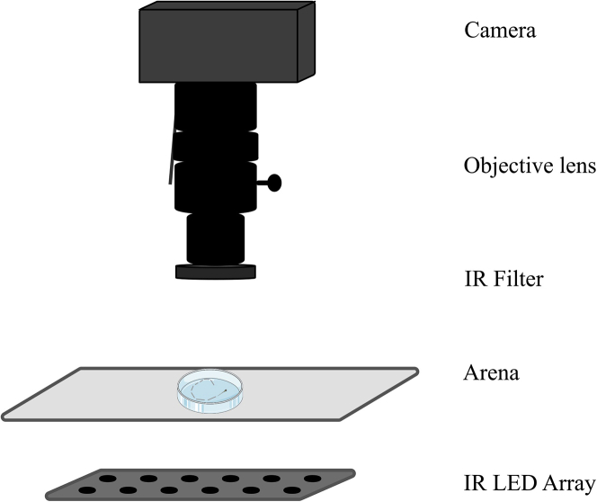
• 3.A brightfield illumination is achieved with an infrared LED array placed below the arena. The distance between the arena and the IR array should be such that it creates a uniform brightfield illumination. An infrared bandpass is used in front of the objective to block all the visible light. The acquisition set-up is illustrated in Figure 1.
• 4.The analysis here focuses on two different swimming patterns, near continuous and intermittent swimming. These are two extremes in the spectrum of swimming patterns employed by fish and hence we believe that this pipeline can be used for comparative analysis of any of the numerous fish species used in the laboratory. To show this, using this set-up, we record several freely swimming Danionella cerebrum (DC) and Danio rerio (ZF) which show a near continuous and an intermittent swimming pattern, respectively. Animal tracking and tail segmentation are performed online using a C# (Microsoft, USA) program published by Marques et al.² The tracking code is available with their publication here, Mendeley Data: https://data.mendeley.com/datasets/r9vn7x287r/1.
• 5.The following method is used by the tracking algorithm²: a background is calculated and subtracted from acquired images. The subtracted image is smoothed using a boxcar filter and an empirically selected threshold is used to separate the fish from the background. The fish silhouette is selected using flood fill starting at the point of maximum intensity. The center of mass of this object defines the larva’s body position. The maximum pixel value on a 0.7 mm diameter circle around this position is used to find the direction of the tail. To refine this measurement, the center of mass is then calculated on an arc centered along this direction. Similarly, several segments are identified by finding the center of mass of the pixel values along a 120-degree arc from the previous segment. To avoid contamination with background noise, pixels below a manually selected threshold level are removed. Please check the above link to access the tracking software.²
• 6.The aforementioned program provides two important parameters for our analysis: the body position coordinates (X, Y) of the fish and the angle of each tail segment. The number and length of segments for the tail can be selected using the tracking program. This depends on the size of the animals used and the length of their tail. In the present study, we keep it at 10 tail segments of 0.3 mm for both the species as their size is very comparable.

CRITICAL: as the raw images are not stored on the disk, before performing the experiments, it is important to make sure that the tail segmentation is correct. For this, some trial data can be acquired where the raw images are also stored along with the fish and tail data. This can be achieved at a lower frame rate without any considerable frame drop. The raw images can then be used to test the reliability of the data extracted online by employing manual segmentation using an image processing tool such as FIJI. In case of errors in the automated segmentation, the user should try to rectify this by 1) making sure that the resolution of the system is 17px/mm or more as described above and 2) improve the contrast between the animal and the background by changing the illumination or exposure time of the camera. These two are the most common sources of error that we have encountered.

Figure 1.

Behavioral imaging set-up

An illustration of the behavioral imaging set-up.

Data cleaning

Timing: 20 min

• 7.The overall input data structure [as obtained from the tracking software] is mentioned here. There are 33 columns. The important variables are described here: 1) frame #, 2) x-position, 3) y-position, 4–5) not applicable for current analysis, 6: head yaw angle, 8) pixel value of detected fish, 9–10) not applicable for current analysis, 11–20) pixel value of tail segments, 21–31) tail segment angles, 32) frame # stamp, 33) frames lagging.

Note: We do not expect the users to have same outputs from the tracking software. If some parameters are not available, we encourage the users to replace the values with NaN. However, it is expected that the information on frame numbers, fish position (x,y) and tail segment angles is always available as these are critical for the analysis.

• 8.
  We identify the following conditions in the data and correct it:

  • a.
    Poor tracking is identified based on pixel intensity information provided by the tracking software (failure to locate the tail results in low pixel values for the detected objects) and replaced with NaN.
  • b.
    Any lost frames are identified based on a number which increments each frame. Lost frames can be interpolated and filled with NaN values for the recorded parameters. If the data is acquired into a circular memory buffer for analysis, then no frames should be lost, unless the analysis lags the acquisition by more than the buffer size.

    % Check for missing frames using frameDiff variable (difference between frames)

    >idx_frame = frameDiff > 1; % index of missing frames

    >idx_lost = find(idx_frame == 1); % first frame in the block of missed frames
  • c.
    Discontinuity in heading orientation can arise when the fish turns from 0 to 360 degree or vice versa. This must be corrected before proceeding further with the analysis of the tail segmentation data. At the recorded framerate changes of more than 180 degrees in either direction over a single frame can be assumed to result from this wrap-around.
  • d.
    Discontinuity in tracking can be another issue. See problem 1 to check how to handle these instances.

    % head yaws

    > headyaw_diff = [nan; diff(headyaw)];

    > headyaw_diff_tmp=headyaw_diff;

    % correction of discontinuities when fish turns from 0 to 2∗pi or vice versa

    > for kk = 1: length(headyaw_diff)

    > if headyaw_diff(kk) > pi % right turn

    > headyaw_diff(kk) = headyaw_diff(kk) - 2∗pi;

    > elseif headyaw_diff(kk) < -pi % left turn

    >  headyaw_diff(kk) = 2∗pi + headyaw_diff(kk);

    > end 

    > end

    headyaw_corr=cumsum(headyaw_diff);

    CRITICAL: The timestamps are important for keeping track of any lost frames during high-speed imaging as many of the parameters we are calculating are time sensitive. The internal timestamp of the camera is most reliable in this respect. In case such a timestamp is unavailable, an alternative way to determine the sampling rate of the camera would be to use a function which checks every incoming image with the previous image and increases a frame counter if the two images are different. This counter can then be used to report the sampling frequency.

Key resources table

REAGENT or RESOURCE	SOURCE	IDENTIFIER
Experimental models: Organisms/strains
Danio rerio (6dpf wildtype larvae)	Fish facility, Institut Curie, Paris	N/A
Danionella cerebrum (6dpf wildtype larvae)	Fish facility, Institut Curie, Paris	N/A
Software and algorithms
MATLAB 2021a	MathWorks (USA)	N/A
MATLAB toolboxes (Signal Processing Toolbox 8.6, Statistics and Machine Learning Toolbox 12, and Statistics and Machine Learning Toolbox 12.1)	MathWorks (USA)	N/A
C# (Microsoft, USA)	Microsoft, USA	N/A
Code for animal tracking and tail segmentation	Marques et al.2	Mendeley Data: https://data.mendeley.com/datasets/r9vn7x287r/1
Other
IR-sensitive Camera (MC1362)	Mikrotron-GmbH, Germany	N/A
Schneider apo-Xenoplan 2.0/35 objective	Jos. Schneider Optische Werke GmbH, Germany	N/A
850 nm infrared bandpass filter (BP850-35.5)	Midwest Optical Systems, Inc.	N/A
IR-LED array	Custom made IR-LED arrays or from local retailer (IR-LED arrays used for night vision cameras).	N/A
Deposited data
Data and code	Generated for this analysis	Mendeley Data: https://doi.org/10.17632/pzwb8dj2hm.1

Step-by-step method details

Using half tail beats to compare short timescale kinematics

Timing: 20 min

This section makes use of the high frequency acquisition data to calculate short timescale (milliseconds) swimming kinematics such as swimming speed, tail beat frequency and tail angle per half tail beat. This provides information about the swim pattern utilized by the larva to achieve the generated thrust. The MATLAB Signal Processing Toolbox 8.6 and Statistics and Machine Learning Toolbox 12 are used in this section. There are a few external functions that we use and provide with this script (Data S1; licenses included wherever applicable). We describe some of the critical or uncommon external functions here:

interp1gap: this function interpolates gaps (by default represented by NaN) in data x when the gaps are smaller than certain sample size of s. This avoids interpolation of large gaps. The default interpolation method is linear but can be changed if needed.³

y = interp1gap(x,s).

txt2mat: this function can carry out automated data analysis on simple text files (decimal number data with common delimiters). Hence, it can be used to import .csv files easily into MATLAB.⁴

Y = txt2mat(name.csv);

round_one: the output (y) is the closest odd number to input (a).

y= round_one(a).

Note: In additional to the external functions that we provide with this publication and describe here, we describe other critical MATLAB functions that are used within the main script when we encounter them. This will make the adaption of this script to any other programing language easier for readers who are more comfortable with another programing language.

• 1.
  Smooth the X and Y coordinates using the Savitzky Golay digital filter.

  Note: In MATLAB, sgolayfilt function is used to carry this out.

  • a.
    Use a 2^nd order polynomial fit on a window of 30 ms.
  • b.
    Calculate the displacement and velocity using the filtered X and Y coordinates of the fish centroid.

    Note:sgolayfilt is a MATLAB function which applies a Savitzky-Golay smoothing filter of nth order polynomial and frame length L to the data in vector x.

    Y=sgolayfilt(x,n,L);
• 2.
  Measure the tail curvature to identify the swim events.²

  • a.
    Select the number of tail segments incorporated in the analysis based on the reliability of tracking available from raw pixel intensities of the segments.
  • b.
    As we want to detect movements, calculate the difference in tail angles.

    • i.
      Calculate the cumulative sum of the angle differences along the tail to capture the change in the overall curvature of the tail over the local fluctuations.

      % unfiltered raw trace

      >dx = [0; diff(xPos)]; % distance between two consecutive x-coordinates

      >dy = [0; diff(yPos)]; % distance between two consecutive y-coordinates

      % prepare for filtering

      >idx_nan = isnan(dx);

      >idx_nan = find(idx_nan==1);

      % filter positions

      >xPos_filt = sgolayfilt(xPos,2,21);

      >yPos_filt = sgolayfilt(yPos,2,21);

      % displacement and velocity

      >dxF = [0; diff(xPos_filt)]; % distance between two consecutive x-coordinates

      >dyF = [0; diff(yPos_filt)]; % distance between two consecutive y-coordinates

      >tmp_dist_filt = sqrt(dxF.ˆ2 + dyF.ˆ2); % distance moved between iterations, in pixels

      >tmp_dist_filt = tmp_dist_filt./camscale_px_per_mm; % convert to distance in mm

      >tmp_vel_filt = tmp_dist_filt.∗datarate_Hz; % convert to velocity in mm/s
• 3.Calculate the absolute value of this accumulated tail curvature so bends in both directions are considered. Smooth this further to give a single measure of curvature. For the zebrafish, based on the available information on bout duration, beat frequency and inter-bout interval, a maximum filter of 28.6 ms is applied to smooth over individual tail beats, and a minima filter of 572 ms is used to calculate and subtract a rolling background to filter out slow changes in tail posture.

%for the bout detection we smooth the tail curvature to eliminate kinks due to tracking noise

>for n=2:size(cumsumtailangles,2)-1

>smoothedCumsumFixedSegmentAngles(:,n)=mean(cumsumtailangles(:,n-1:n+1)');

>end

%we consider the difference in segment angles, because we want to detect tail movement

>fixedSegmentAngles = [zeros(size(cumsumtailangles,2),1)'; diff(smoothedCumsumFixedSegmentAngles)];

%Filter angles

>bcsize=14; %this parameter sets the timescale at which to smooth the tail movement

>filteredSegmentAngle = realSegmentAngles∗0;

>for n = 1 : (size(realSegmentAngles,2)) %smooth the tail movements at the shorter timescale

>filteredSegmentAngle(:,n) = conv(realSegmentAngles(:,n),ones(bcsize,1)'/bcsize,'same');

>end

%we sum the angle differences down the length of the tail to give prominence to regions of continuous curvature in one direction

>cumFilteredSegmentAngle = cumsum(filteredSegmentAngle')';

%we sum up the absolute value of this accumulated curvature so bends in both directions are considered

>superCumSegAngle = cumsum(abs(cumFilteredSegmentAngle)')';

%Calculate tail curvature; it convolves all segments in one

>bcFilt=14; tailCurveMeasure = conv(superCumSegAngle(:,end), ones(bcFilt,1)'/ bcFilt, 'same');

• 4.Identify the start and end of swimming bouts/events based on empirically selected cut-offs in both the species.

Note: The cut-offs should work well across various swim types and species if the data is not very noisy.

% tailCurveMeasure is filtered more and smootherTCM is the resultant filtered curvature measure

>allbout= smootherTCM>0.13; %empirically selected threshold for one of the species

>allstart=max([0 diff(allbout')],0);

>allend=max([0 -diff(allbout')],0);

• 5.
  Now, detect the half tail beats in the identified swim events.

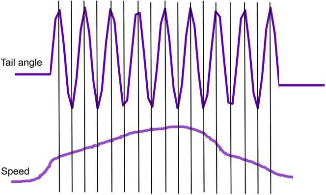
  • a.
    Define a half tail beat as a peak-to-peak half cycle and use this to calculate the short timescale swimming kinematics (Figure 2).
  • b.
    To identify half tail beats, calculate the absolute value of the tail angle signal and then identify the peaks. In MATLAB, the peaks are identified using the findpeaks function.

Note:findpeaks is a MATLAB function that identifies local maxima (peaks) in the input vector (data). It also returns the indices (locs) of the identified peaks.

Figure 2.

Identification of half tail beats

Illustration of dissection of a swim event into half tail beats for calculation of short timescale swim kinematics.

[peaks, loc] = findpeaks(data).

• 6.Using this information about peaks, calculate the kinematic parameters like swim duration, distance, mean and maximum speed, maximum tail angle and half beat frequency on the individual half tail beats.

>for swm = 1 : length(starts) %go through each swim event

>tmp_forTBF_intrp=forTBF_intrp(starts(swm):ends(swm));

>[pks_tmp,locs_tmp]=findpeaks(abs(tmp_forTBF_intrp),'MinPeakProminence',thresholdBeats,'MinPeakDistance',cutOff); %ID all half beats; swim pattern specific thresholds are provided

>IDfalsePeaks=locs_tmp(forVeloFilt_intrp_filtfilt(locs_tmp)<1);

>locs_tailPeaks=setdiff(locs_tmp,IDfalsePeaks);

>beatStarts=[locs_tailPeaks(1:end-1)];

>beatEnds=[locs_tailPeaks(2:end)];

> for nHBT=1:length(beatStarts) %go through each half beat

  %calculate all the half beat based kinematics here.

> end

>end

CRITICAL: The filtering is carried out to remove high frequency noise. It is a good practice to compare the filtered signal against the unfiltered signals to make sure that only the high frequency noise is removed, and no artefacts are introduced because of the filtering process. While the selection of filters can vary based on the signal, we share two separate kinematic analysis scripts (see Data S1) for analysis of intermittent and continuous swimming patterns. This is expected to apply to a variety of species with differing swim patterns. The user is expected to select the script based on whether the animal’s navigation fits an intermittent or continuous swimming pattern (see problem 2).

Using mean square displacement and heading decorrelation to compare long timescale kinematics

Timing: 20 min

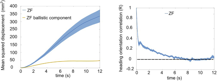
This section only uses low frequency acquisition data (or down sampled high frequency data) to compute the mean square displacement (MSD) and heading persistence (R) as a function of time. R(Δt) is defined as the mean dot product of the heading vectors computed at time points separated by a delay Δt. The heading persistence thus characterizes how the correlation in heading orientation is progressively lost as the animal explores its environment. A purely ballistic (straight) movement correspond to R=1 for any delay. Reversely, for a purely diffusive process, R immediately decays to zero. Together, these two quantities characterize the spatial and angular dynamic underlying the long timescale (seconds) exploration of the fish.

This section makes use of the MATLAB Signal Processing Toolbox 8.6, Statistics and Machine Learning Toolbox 12, and Statistics and Machine Learning Toolbox 12.1.

• 7.Apply a Savitsky-Golay filter on the X/ Y traces to fit a 2^nd order polynomial on a 200 ms window.
• 8.Down sample the filtered trajectories to 70 Hz.

Note: This is done as our original sampling rate was 700 Hz. Perform this step only if it applies to your acquisition.

>x=dt(n).xPos;

>y=dt(n).yPos;

downsample=70; % data are downsampled by this factor for the analysis.

>x=sgolayfilt(x,2,2∗downsample+1); % filter trajectories over twice the sampling window

>y=sgolayfilt(y,2,2∗downsample+1);

>x=x([1:downsample:end]); % downsample

>y=y([1:downsample:end]);

>w=find(((x-center(1)).ˆ2+(y-center(2)).ˆ2)>Radiusˆ2); % detect positions too close to the border

>IndIn=ones(length(x),1);

>IndIn(w)=0; % IndIn is one when the fish is inside the ROI, zero otherwise

dt_v=2; % time interval over which to compute heading orientation (in number of tau)

delta=[0:1:200]; % time indices at which we evaluate MSD (i.e., 0 to 20 s every 0.1 s)

• 9.Identify discrete continuous trajectories in a circular region within the arena (Figure 3). In doing so, we remove parts of the trajectories close to the border of the dish which may affect the exploratory dynamics of the fish.
• 10.Every 100-ms time step, calculate the time-evolution of MSD and R over all the identified trajectories.

% separate the data into a discrete collection of trajectories within the ROI

>[L,Ntraj]=bwlabel(IndIn); % Ntraj is the number of trajectories

>Ltraj=zeros(Ntraj,1); % Ltraj gives the length of each trajectory

>for traj=1:Ntraj;

> Ltraj(traj)=length(find(L==traj));

>end

>Xsp=NaN(Ntraj, max(Ltraj)); % x,y position split in trajectories

>Ysp=NaN(Ntraj, max(Ltraj));

>theta=NaN(Ntraj, max(Ltraj)-dt_v); % heading orientation

>Npoints_dt(n)=length(find(IndIn==1 & isnan(x)==0));

% The X and Y positions vectors are split into separate trajectories defined as uninterrupted periods during which the animal remains in the ROI : Xsp(i,j) is the X coordinates for the ith trajectory at time j counted from the onset of this particular trajectory.

>for traj=1:Ntraj;

> Xsp(traj,1:Ltraj(traj))=x(find(L==traj));

> Ysp(traj,1:Ltraj(traj))=y(find(L==traj));

% Same computation is performed for the heading vector [dX,dY]. The heading angle is only computed when the animal has moved over at least 10 pixels over 1 s.

> dXsp=Xsp(traj,(dt_v+1):end)-Xsp(traj,1:end-dt_v);

> dYsp=Ysp(traj,(dt_v+1):end)-Ysp(traj,1:end-dt_v);

> w=find(dXsp.ˆ2+dYsp.ˆ2)>100;

> theta(traj,w)=atan2(dYsp(w),dXsp(w));

• 11.To calculate R (heading persistence), if the fish moves at least 0.5 mm, extract at each time t a unit vector u(t) aligned along the fish displacement [dx, dy] calculated over a 1 s time window.
• 12.Compute the heading decorrelation over a period Δt as R(Δt)=<u(t).u(t + Δt)>_t.

% First we calculate the MSD. we successively compute the mean displacement travelled over time delay delta(k).

>for k=1:length(delta);

>  p=delta(k);

>  dx=Xsp(:,(p+1):end)-Xsp(:,1:end-p);

>  dy=Ysp(:,(p+1):end)-Ysp(:,1:end-p);

>  MSD(k,n)= nanmean(dx(:).ˆ2+dy(:).ˆ2); % recall n is the fish index

% we also compute the standard error of the mean for each time delay

>  Ndata=sum(isfinite(dx(:))==1);

>  if Ndata >=1;

>  semMSD(k,n)=nanstd(dx(:).ˆ2+dy(:).ˆ2)/sqrt(Ndata);

>  end

% The heading persistence, i.e., the mean of the heading vectors dot product, is computed as the cosine of the reorientation angle dtheta

>  dtheta=theta(:,(p+1):end)-theta(:,1:end-p);

>  R(k,n)=nanmean(cos(dtheta(:)));

>  

>  Ndata=sum(isfinite(dtheta(:))==1);

>end

• 13.R quantifies the heading persistence in a given time period. R = 1 indicates a perfect maintenance of the heading orientation, whereas R = 0 indicates a complete randomization of the orientation.

Figure 3.

Identification of discrete swim trajectory

Illustration of discrete swim trajectories identified for calculation of long timescale swim kinematics. An example trajectory is highlighted in red. The ROI (dark grey) is used to avoid border-induced bias in the swimming activity.

Expected outcomes

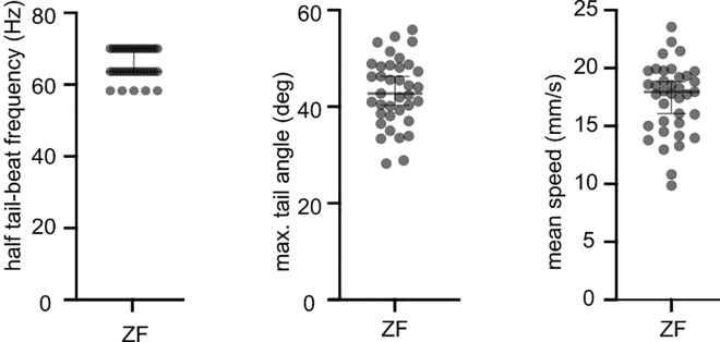
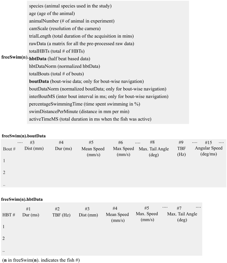
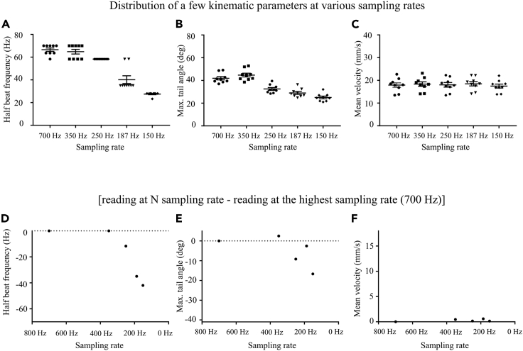
The short timescale kinematics (Figure 4) shows how tail beat frequency and maximum tail angle concur to produce a certain swimming speed. This is useful to compare between fish species to understand the differences or similarity in their short timescale kinematics. Moreover, we provide the structure of the output data in Figure 5. The short timescale analysis requires high frame rate as highlighted before. We reanalyzed the data set on down sampled data and found the results to be very poor for half tail beat frequency or maximum angles when the sampling rate was below 350 Hz (Figure 6).

Figure 4.

Short timescale kinematics

The short timescale kinematics (half tail beat frequency, maximum tail angle and speed) helps us to understand how the thrust for swimming is achieved by using tail movements. The error bars indicate SEM.

Figure 5.

Output data structure of short timescale analysis

The structure of output data produced by the short timescale analysis pipeline. The bout-based parameters are specific to intermittent swimming.

Figure 6.

Short timescale analysis of downsampled data

(A–C) show distribution of results obtained for half beat frequency, maximum tail angle and mean velocity, respectively after down sampling the data. The downsampled sampling rates are shown. The error bars indicate SEM.

(D–F) show the change in estimation of the parameter when compared with the result obtained at 700 Hz. The maximum value on the y-axis corresponds to the mean of the respective parameter for the sample set.

The long timescale kinematics (Figure 7) informs us about the navigational strategy used by the animal to explore its environment. MSD gives a measure of the area explored by the animal in a given time and R (heading persistence) quantifies the time evolution of reorientation kinematics. As highlighted before, this analysis will work robustly even when the sampling rate is very low. In Figure 8, we perform the same analysis on the raw data down sampled to 70 Hz and find the results to be very similar to the one obtained with processed data obtained at 700 Hz.

Figure 7.

Long timescale analysis

The long timescale kinematics helps us to understand how the animal explores its environment by looking at the reorientation kinematics. The error bars indicate SEM.

Figure 8.

Long timescale analysis of raw down sampled data

The (A) mean square displacement (MSD) and (B) heading decorrelation (R) obtained by using the data collected and filtered at 700 Hz compared with results obtained from raw data downsampled at 70 Hz. The error bars indicate SEM.

Overall, this analysis approach lets us compare how both short- and long- timescale factors interact with each other in various larval species to produce their natural exploratory behavior.

Limitations

As the short timescale kinematics is carried out per half tail beat, it is essential to have a high frequency acquisition system to be able to do capture half tail beats. In order to reliably track the amplitude and shape of tail beats, the recording should be made at several times greater than the fundamental frequency of the signal that one is trying to analyze. At the Nyquist sampling level (2 × the fundamental frequency) movement peaks may not be detected depending on the sampling phase. In the cases of escape behavior, this can be over 500 Hz in some fish species. Availability of such a high-speed acquisition system can often be a limitation. We used the higher frequency signal of zebrafish larvae (compared to Danionella) to determine this limit in free swimming larval fish data and found a sampling rate >350 Hz to be essential in this case.

Another limitation arises from the fact that we do not include the role of fins in locomotion in our analysis.⁵ To be able to incorporate the fin movements, one would have to use a tracking system with much higher spatial resolution, and this often comes at the cost of decreased temporal resolution.

Troubleshooting

Problem 1

Discontinuity in animal tracking is often a problem as animals show thigmotaxis wherein they tend to occupy the edges of the behavioral arena. At the edges, poor illumination can cause an unreliable tracking.

Potential solution

One can correct for this issue before data acquisition by using optical or behavioral methods such as use of a curved arena or use of positive/ negative phototactic ring at the edge to force animal to spend more time in the center. If one is unable to correct for the issue before data collection, they will have to take care of this during the data processing. As mentioned in the protocol, we do this in our analysis using two different approaches. In short time scale analysis, we use the pixel value information to discard the poor tracking events from the dataset [see step 8 in before you begin]. In the long timescale analysis, we select trajectories in a region of interest in the arena which excludes the borders of the arena where poor illumination leads tracking errors [see step 9 in step-by-step method details]. The small gaps in tracking can then be interpolated.

Problem 2

Subtle species to species variations.

Potential solution

Species to species variation in pigmentation can often lead to differences in the thresholds required for binarization of the fish image and segmentation. We recommend selecting the threshold empirically based on the species-to-species variation in pigmentation. Such subtle differences even in the same tracking system can introduce unexpected noise in the tracking data between different species. So, despite the consistent overall analysis approach between different larval species, there might be some parameters which will have to be selected empirically based on the species and its signal-to-noise (SNR) ratio in the tracking data. The easiest solution to this is to make sure that the tracking data has high SNR by selecting the best possible thresholds for fish segmentation in the tracking software. This can be done by visual inspection by comparing the contrast between the animal and the background. The tracking software referred to in this protocol also provides this function to change the threshold value by manual visual inspection [see step 4 in before you begin].

Resource availability

Lead contact

Further information and requests for resources and reagents should be directed to and will be fulfilled by the lead contact, Filippo Del Bene (filippo.del-bene@inserm.fr).

Materials availability

This study did not generate new unique reagents.

Data and code availability

The original analysis scripts and example datasets generated during this study are deposited to Mendeley Data: https://doi.org/10.17632/pzwb8dj2hm.1.

References

- 1.Rajan G., Lafaye J., Faini G., Carbo-Tano M., Duroure K., Tanese D., Panier T., Candelier R., Henninger J., Britz R., et al. Evolutionary divergence of locomotion in two related vertebrate species. Cell Rep. 2022;38:110585. doi: 10.1016/j.celrep.2022.110585. [DOI] [PubMed] [Google Scholar]
- 2.Marques J.C., Lackner S., Félix R., Orger M.B. Structure of the zebrafish locomotor repertoire revealed with unsupervised behavioral clustering. Curr. Biol. 2018;28:181–195.e5. doi: 10.1016/j.cub.2017.12.002. [DOI] [PubMed] [Google Scholar]
- 3.Greene C. interp1gap. 2022. https://www.mathworks.com/matlabcentral/fileexchange/45842-interp1gap MATLAB Central File Exchange.
- 4.Andres txt2mat. 2022. https://www.mathworks.com/matlabcentral/fileexchange/18430-txt2mat MATLAB Central File Exchange.
- 5.McClenahan P., Troup M., Scott E.K. Fin-tail coordination during escape and predatory behavior in larval zebrafish. PLoS One. 2012;7:e32295. doi: 10.1371/journal.pone.0032295. [DOI] [PMC free article] [PubMed] [Google Scholar]
Associated Data
This section collects any data citations, data availability statements, or supplementary materials included in this article.
Supplementary Materials
Data Availability Statement