Spatial intra-tumor heterogeneity is associated with survival of lung adenocarcinoma patients

Summary

Intra-tumor heterogeneity (ITH) of human tumors is important for tumor progression, treatment response, and drug resistance. However, the spatial distribution of ITH remains incompletely understood. Here, we present spatial analysis of ITH in lung adenocarcinomas from 147 patients using multi-region mass spectrometry of >5,000 regions, single-cell copy number sequencing of ∼2,000 single cells, and cyclic immunofluorescence of >10 million cells. We identified two distinct spatial patterns among tumors, termed clustered and random geographic diversification (GD). These patterns were observed in the same samples using both proteomic and genomic data. The random proteomic GD pattern, which is characterized by decreased cell adhesion and lower levels of tumor-interacting endothelial cells, was significantly associated with increased risk of recurrence or death in two independent patient cohorts. Our study presents comprehensive spatial mapping of ITH in lung adenocarcinoma and provides insights into the mechanisms and clinical consequences of GD.

Graphical abstract

Highlights

• •Lung adenocarcinomas show “random” or “clustered” GD
• •Random GD tumors have significantly poorer survival
• •Random GD tumors are characterized by decreased cell adhesion
• •Clustered GD tumors have high levels of tumor cell-interacting endothelial cells

Using three orthogonal spatially resolved molecular profiling technologies, Wu et al. identified two groups of lung adenocarcinomas with distinct patterns of geographic diversification. They found that these two groups differed in their survival outcomes and found evidence suggesting that the observed patterns may be linked to differences in tumor cell motility.

Introduction

Lung cancer is the most common type of cancer and the leading cause of cancer death worldwide.¹ Lung adenocarcinoma, the most frequent subtype of non-small cell lung cancer (NSCLC), is characterized by heterogeneity among individual tumors² and between regions in a single tumor.³ The heterogeneity between regions, termed intra-tumor heterogeneity (ITH), has been shown to contribute to treatment failure and drug resistance through the expansion of pre-existing resistant subclones and their derivatives.4, 5, 6, 7 For example, EGFR T790M-positive cells are observed in response to the treatment of NSCLC with EGFR tyrosine kinase inhibitors.⁷ Furthermore, several studies have shown that certain patterns of ITH, mostly measured in terms of the subclonal alteration burden, are associated with poor clinical outcomes in multiple cancer types including NSCLC.^3,8, 9, 10 Previous studies have attempted to decode the spatial patterns of such heterogeneity using multi-region profiling.^3,11, 12, 13, 14, 15 However, the small number of regions analyzed per tumor limits the conclusions of these studies. This caveat has resulted in major gaps in our understanding of spatial tumor heterogeneity and its contribution to tumor progression and the organization of the tumor-immune ecosystem,16, 17, 18 which is particularly important in light of the recent success of immune checkpoint blockade.¹⁹

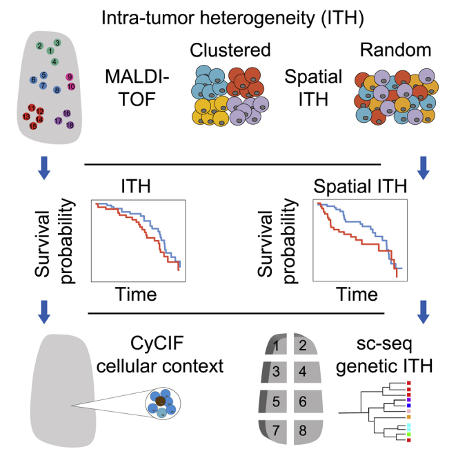
Here, we present a large-scale, integrative analysis of ITH and its spatial organization in lung adenocarcinoma based on multiple orthogonal methods that are able to profile multiple regions and/or single cells across a tumor sample while preserving their spatial context. These analyses include multi-region MALDI-TOF (matrix-assisted laser desorption ionization-time of flight) of ∼5,000 regional spectra from 147 patients in two independent cohorts (Figure 1A), CyCIF (cyclic immunofluorescence) of >10 million cells from 12 patient samples (Figure 1A), and multi-region single-cell copy number sequencing of ∼2,000 single cells from 51 regions of 7 patient samples (Figure 1C). These data aim to elucidate the extent of ITH and its spatial pattern in both proteomic and genomic spaces in lung adenocarcinoma and to explore how such spatial heterogeneity variation across patients is associated with the tumor microenvironment and copy number variation, and how it influences clinical outcomes.

Figure 1.

Overview of methods used to investigate intra-tumor spatial heterogeneity in this study

(A) Overview of multi-region MALDI-TOF.

(B) Overview of cyclic immunofluorescence.

(C) Overview of multi-region single-cell copy number sequencing.

Results

Multi-region MALDI-TOF analysis of lung adenocarcinomas

To study spatial heterogeneity of lung adenocarcinomas in the proteomic space, we sectioned resected frozen human lung adenocarcinoma specimens and collected paired neighboring sections for each biopsied specimen—one for the identification of histologic patterns of tumor cells or normal alveolar and bronchial epithelial tissues, and one for MALDI-TOF profiling. Intratumoral histologic subtypes that could be identified included lepidic, acinar, papillary, micropapillary, solid, complex gland, and cribriform types.²⁰ Areas from these various intratumoral histologic subtypes were selected for mass spectrometry profiling such that each site yielded a spectral profile and its geographic location within the tumor section (Figure 1A). All tumor sections were obtained from the largest cross-sections of a given tumor, and the best effort was made to sample the entire section for unambiguous representatives of the seven classic histologic categories mentioned above.²⁰ An example of a histologic annotation is shown in Figure 2A. In the discovery cohort, we collected 4,007 regions of interest (ROIs) (diameter 200 μm) from 95 patients, with an average of 30 tumor spectra and 12 normal spectra per patient (Figure 2B). Furthermore, three mesenchymal stem cell (MSC) and three basal stem cell samples were profiled to obtain stem cell protein expression profiles as a reference for further analysis, since the molecular distance of a cancer sample from stem cells was found to be associated with worse outcome in multiple cancer types.²¹ A range of 110–935 spectra was profiled for each sample across different histologic subtypes (Figure S1A). For each regional sample, a total of 525 protein peaks were identified, and the signal intensities of the peaks were integrated to capture the expression levels of individual proteins (see STAR Methods and Figure 1A).

Figure 2.

Proteomic spatial heterogeneity in lung adenocarcinoma

(A) Example of histologic annotation and sample profiling.

(B) Number of normal and tumor spectra profiled in patients from the discovery cohort.

(C) Proposed patterns of intra-tumor GD.

(D) Illustration of a clustered GD pattern (patient P137149). Left panel: geographic locations of regional samples and their nearest neighbors in proteomic space. Right panel: scatterplot of geographic and molecular distances. Each dot represents a pairwise distance between two regional samples. R, Mantel correlation coefficient; P, Mantel test p value.

(E) Illustration of a random GD tumor (patient P132654). Left panel: geographic locations of regional samples and their nearest neighbors in proteomic space. Right panel: scatterplot of geographic and molecular distances. Each dot represents a pairwise distance between two regional samples. r, Mantel correlation coefficient; P, Mantel test p value.

(F) Kaplan-Meier survival curves shown for patients with clustered and random GD patterns from the discovery cohort. Patients with random GD patterns had significantly worse outcomes than those with clustered GD patterns. HR, hazard ratio; P, log-rank p value. Clustered and random GD patterns are defined in Figure S3D. Multivariate Cox proportional hazards regression analysis with continuous GD score by controlling for clinicopathological risk factors are shown in Table S3.

(G) Number of normal and tumor spectra profiled in patients from the validation cohort.

(H) Kaplan-Meier survival curves shown for patients with clustered and random GD patterns from the validation cohort. Patients with random GD patterns had significantly worse outcomes than those with clustered GD patterns. HR, hazard ratio; P, log-rank p value. Clustered and random GD patterns are defined in Figure S3F. Multivariate Cox proportional hazards regression analysis with continuous GD score by controlling clinicopathological risk factors are shown in Table S5.

(I) Growth pattern presence in clustered and random GD tumors. The y axis shows the base 2 logarithm of the odds ratio from Fisher’s exact test when comparing the number of clustered and random tumors with at least one sample for the indicated growth patterns. Values < 0 indicate that random GD tumors are less likely to have a region with the indicated growth pattern. The points represent estimates while the bars represent the 95% confidence interval. N.S., not significant.

(J) Grade of clustered and random GD tumors. Fisher’s exact test p value is shown.

Distance matrix-based principal-component analysis (PCA) demonstrated a continuous trajectory in proteomic space from normal lung tissue to tumor to stem cells, the latter being farthest away from normal lung tissue (Figure S1B). There was no clear separation between different histologic subtypes, neither in a single patient nor when all patients were considered as a set (Figures S1B and S1C); this was also true for transcriptomes in The Cancer Genome Atlas dataset.² There were no notable proteins that showed histology-specific expression. However, clear differences were observed between tumor and normal tissues with regard to their differentially expressed proteins, and these gave rise to an intermediate cluster (Figures S1D and S1E) that contained a large proportion of normal samples and low-grade histologies, and a low proportion of more clinically aggressive histologies except for micropapillary (Pearson’s correlation coefficient = −0.72; p < 0.05).²⁰ When the trajectory of samples was further investigated relative to MSC and normal differentiated tissues in PCA space, the most aggressive histologies (such as solid) clustered with MSCs, whereas the least-aggressive subtypes (such as lepidic) clustered with normal differentiated tissues (Figure S1B).

Proteomic ITH in lung adenocarcinoma

We next sought to investigate the extent of ITH in proteomic space using MALDI data. The Shannon index (a measure of entropy) has previously been used to quantify the degree of ITH in tumors when the “species” (cells or samples with unique features) are clearly identifiable.²² However, such species are usually unobtainable in systematic studies of the whole tumor proteome or transcriptome. We recently used mean cell-to-cell distance for quantifying ITH based on single-cell RNA sequencing (RNA-seq) data.²³ Here, we defined a similar metric, the scaled mean pairwise distance (sMPD), to quantify ITH across regional samples from patient samples present in the MALDI dataset (Figures S2A and S2B). To test the accuracy of this metric in the setting of MALDI data, we performed a simulation study to compare sMPD with the true ITH quantified by Shannon or Simpson indices by using subclonal information (see STAR Methods; subclonal information is blind to the sMPD calculation). We obtained a high prediction accuracy of sMPD (Figures S2C and S2D; receiver operating characteristic area under the ROC curve ranging from 0.8 to 0.99). Down-sampling analysis demonstrated that the sMPD is robust to sample size (Figure S2E; all samples had an ITH rank change less than 10% when the sample size was larger than 10). We found a trend between higher ITH, as quantified by sMPD, and increased risk of patient death (Figure S2F; p = 0.063, log-rank test); this association was non-significant when controlling for known clinicopathological risk factors (Tables S1 and S2; p = 1, Cox proportional hazards model with continuous sMPD).

We next investigated the spatial organization of ITH—the geographic diversification (GD) of samples in proteomic space. A variety of approaches have been proposed to study spatial patterns of the proteome and transcriptome.^24,25 However, these methods were not designed to quantify intra-tumor spatial heterogeneity by integrating all measured features in a spatially resolved manner. We therefore designed a novel analysis approach: we defined GD to be a measure of the association between molecular features and geographic locations, quantified using the Mantel correlation test²⁶ (see STAR Methods). Tumors can have one of two GD patterns: a clustered pattern, in which molecularly similar cells are clustered together in space, or a random pattern, in which molecularly similar cells are randomly distributed in space (Figures 2C and S3A). When applied to our data, the Mantel correlation test provides the extent of correlation and its significance between the pairwise molecular distances obtained from protein expression patterns and the pairwise geographic distances (Figure S3B). We again used down-sampling analysis to demonstrate the robustness of this metric (Figure S3C; all samples had a GD rank change less than 10% when sample size was larger than 20). We identified two groups of tumors: those whose Mantel correlations were significantly positive and those whose correlations were non-significantly different from zero (p value cutoff: 0.01; Figure S3D). To compare our findings with those obtained using an existing approach, we clustered the ROIs within each tumor sample based on their MALDI profile using PhenoGraph²⁷ and visualized the spatial distribution of different proteomic clusters (Figure S3E). We found that ROIs from the same proteomic clusters tended to be localized close to each other in clustered GD tumors, while the ROIs from the different proteomic clusters tended to intermix in random GD tumors. Quantification of this pattern obtained using PhenoGraph showed a significant difference between clustered and random GD tumors as defined by the Mantel test (p = 0.00041, Wilcoxon test; Figure S3F). Together, our observations demonstrate that tissues with similar protein composition were spatially co-localized in clustered GD tumors and more evenly distributed in random GD tumors. Representative tumors from each group are shown in Figures 2D and 2E. We then investigated overall survival times of patients within these two groups, observing that the random GD pattern was significantly associated with an increased risk of patient death (Figure 2F; p = 0.008, log-rank test); this association was robust when controlling for clinicopathological risk factors in a multivariate Cox proportional hazards regression analysis, and was not dependent on the GD cutoff (Table S3; p = 4.41E–08, hazard ratio (95% CI) = 3.17 (2.10–4.79), Cox proportional hazards model with continuous GD).

To validate this finding, we performed MALDI TOF analysis on a validation cohort of 52 additional patients (1,016 additional ROIs with a diameter of 200 μm; Figures 2G, S3G, and S3H). The validation cohort was generated after all analyses on the discovery cohort were completed. In this validation cohort, we focused on the patient progression-free survival (PFS) because of the low number of death events, and detected the same trend as in the discovery cohort between GD patterns and patient PFS using Kaplan-Meier analysis (Figure 2H; p = 0.099, log rank test). Multivariate Cox regression analysis further showed that the random GD pattern was significantly associated with increased risk of PFS after adjusting for known clinicopathological risk factors, and was not dependent on the GD cutoff (Tables S4 and S5; p = 0.0038, hazard ratio (95% CI) = 1.36 (1.10–1.67), Cox proportional hazards model with continuous GD). Further analysis of overall survival demonstrated that GD patterns were also significantly associated with patient death in a multivariate Cox regression analysis even though the number of deaths was low in this cohort (Tables S4 and S6; p = 0.017, hazard ratio (95% CI) = 1.35 (1.05–1.73), Cox proportional hazards model with continuous GD).

Sample covariates are associated with GD patterns

To gain further insight into the etiology of the observed spatial patterns, we investigated the correlation between random GD and sample covariates in the discovery cohort. Patients with random GD tumors did not differ significantly in terms of smoking history, type of adjuvant treatment, tumor size, stage, or the number of regional tumor or normal samples. However, the total number of regional samples from random GD tumors was smaller (p = 0.012, Wilcoxon test; Figures S4A–S4E). Furthermore, random GD tumors less frequently contained samples with the acinar growth pattern (p = 0.001, Fisher’s exact test; Figures 2I and S4F), and were more frequently high grade (p = 0.02, Fisher’s exact test; Figure 2J). Out of the total number of samples, the presence of acinar histology, and grade, only grade was significantly associated with survival in univariate analysis (p = 0.03; Figures S4G–S4I). Importantly, the association between GD and survival remained significant when grade was included as an additional variable in the Cox proportional hazard’s model (p = 1.02E–7), while grade was not significant (p = 0.94 and p = 0.52, grade 2 and 3 versus grade 1, respectively). These findings suggest that GD is related to tumor grade, but that GD contains additional information relevant to outcome beyond the information encoded by grade.

Intercellular heterogeneity in normal tissue adjacent to tumor

A recent study revealed that normal tissue adjacent to tumor (NAT) exhibits a transcriptional program intermediate between normal tissue (that is distant from the tumor) and the tumor itself.²⁸ Due to this observation, we sought to quantify intercellular NAT heterogeneity in proteomic space. NAT was selected as normal bronchioles or normal alveolar tissue within a distance of 0.1–0.5 cm from the tumor and profiled as above. We did not detect a significant association between tumor and NAT samples in terms of ITH (Pearson’s r = 0.289, p = 0.0568; Figure S5A) and GD (Pearson’s r = 0.07, p = 0.65; Figure S5B). In addition, NAT GD was not significantly associated with overall survival (Figure S5C).

Transcriptional programs associated with GD

We hypothesized that the different patterns of GD—clustered versus random—observed in MALDI data might reflect different degrees of cellular motility in these tumors. To test this hypothesis and to study the transcriptional programs associated with different GD patterns, we performed bulk RNA-seq on 53 tumors from the discovery cohort. We found that cell-cell adhesion-related pathways, such as cadherin binding (NES = −2.16; q = 0.05), transmembrane transport (NES = −2.32; q = 0.04), and extracellular matrix genes (NES = −2.27; q = 0.05) were the top enriched gene sets, with significantly lower expression in tumors of a random, as opposed to clustered, GD pattern (Figure S6A; Table S7). Reduced expression of cadherin family genes is related to a decrease in cell-cell adhesion and can promote cell migration and invasion,²⁹ which might contribute to the random GD pattern in tumors (Figure S6B). Alternatively, reduced expression of cell adhesion markers in random GD tumors could reflect a decrease in epithelial cell content in these samples. However, detailed functional studies are required to validate whether cell-cell adhesion pathway genes are indeed associated with different GD patterns, and to determine the mechanistic basis of this result, in a large sample set. In contrast, random GD tumors showed an increased expression of genes related to immune response pathways as the top regulated gene sets (Figures S6C and S6D; Table S7), although this finding was not statistically significant.

Since it has previously been demonstrated that immune infiltration is associated with patient outcome in primary tumors,^16,30,31 we hypothesized that immune activation may be implicated in the formation of random GD tumors. To test this hypothesis, we utilized the RNA-seq data to estimate the proportion of various immune cell types by using a signature^32,33 that had previously been applied to NSCLC.³¹ This signature consists of ∼60 marker genes whose expression levels measure 14 immune cell populations (see STAR Methods). The inferred proportions of different immune cell types were correlated with estimates based on CyCIF imaging of the same samples (see next section; average Pearson’s r = 0.72, range from 0.32 to 0.95 for different immune cells; Figure S7A). We found that none of the immune infiltrates, except neutrophils (p = 0.03, Wilcoxon test), were associated with ITH (Figure S7B). In contrast, the number of CD8⁺ T cells were significantly associated with random GD tumors (Figure S7C; p = 0.036, Wilcoxon test), with other infiltrating immune cells, such as B cells, natural killer cells, and regulatory T cells showing the same trend albeit not statistically significant. Further analysis showed that the proportions of different immune cell types were not associated with overall patient survival (Figure S8A; p > 0.05, Cox proportional hazards model), indicating that GD is more significantly associated with overall survival than the extent of immune cell infiltration estimated from bulk RNA-seq data, even though GD may be partly driven by immune cell composition.

To characterize the repertoire of T and B cell receptors in clustered and random GD tumors, we applied the RNA-seq Immune Analysis (RIMA) (https://kateyliu.github.io/RIMA/index.html) pipeline to our bulk RNA-seq data. We found no significant difference in statistics quantifying the level of B cell somatic hyper-mutation or T and B cell receptor diversity (p > 0.05, Wilcoxon tests; Figures S9A and S9B). However, we found that random GD tumors had a significantly higher fraction of B cell receptor reads (p = 0.044, Wilcoxon test; Figure S9A), consistent with our earlier result suggesting higher levels of B cell infiltration in random GD tumors compared with clustered GD tumors. The fraction of T cell receptor reads was higher in random GD tumors than clustered tumors, but the difference was not significant (Figure S9B). Taken together, these results indicate that the formation of random GD tumors is associated with a combination of repression of cell adhesion and increased immune infiltration.

Tumor cellular composition and microenvironmental interactions

To further characterize tumor composition and spatial interactions between tumor and microenvironmental cells, such as infiltrating immune cells, endothelial cells, and mesenchymal cells, we performed multiplexed tissue imaging by CyCIF using antibodies against KERATIN, CD45, PCNA, CD8A, CD3D, CD4, KI67, PD1, CD163, CD11C, FOXP3, CD20, VIM, CK7, GZMB, CMA1, CD31, and S100A11 on 12 tumors from the discovery cohort. We sectioned resected, formalin-fixed, paraffin-embedded tumors and collected paired neighboring sections for each biopsied specimen—one for conventional H&E staining for histopathological analysis and one for CyCIF (Figure 1B). Paired images were overlaid (Figures 3A and 3B), regions of interest were identified based on histological patterns, and corresponding cells in the CyCIF image were then segmented and quantified based on whole-cell fluorescence intensity (see STAR Methods). Since S100A11 expression was measured by both CyCIF and MALDI, we used this marker to compare across orthogonal methods and observed correlation between the two methods across patients (Pearson’s r = 0.77, p = 0.0031; Figure S10A).

Figure 3.

The tumor-immune landscape associated with proteomic spatial heterogeneity

(A) Example images of H&E and immunofluorescence of a representative patient biopsy.

(B) Example images of H&E and immunofluorescence of representative histological regions. First row, H&E image; second row, immunofluorescence image; third row, single-cell quantification results; fourth row, cell type classification results; 200 × 200 μm regions are shown, which represent the same sized regions as in MALDI data.

(C) t-SNE plot on 5% of all single cells profiled by CyCIF. The upper panel shows the dimensional reduction results of all identified cells; t-SNE was performed on all proteins except S100A11. The lower panel shows the dimensional reduction results of all identified immune cells; t-SNE was performed on the immune markers CD45, CD8A, CD3D, CD4, CD163, FOXP3, CD20, CMA1, CD11C, PD1, and GZMB.

(D) Inter- and intra-tumor heterogeneity with respect to immune cell infiltration. Upper panel: the proportion of different cell types in each tumor specimen. Lower panel: the proportion of different immune cell types in each tumor specimen.

(E) Correlation between proteomic GD and percentage of immune-interacting tumor cells.

(F) Correlation between proteomic GD and percentage of tumor-interacting endothelial cells.

(G) Correlation between proteomic GD and percentage of tumor-interacting mesenchymal cells.

(H) Examples of patient biopsies with high and low frequencies of tumor-interacting endothelial and mesenchymal cells. Imm., immune cells; Non-tumor Epi., non-tumor epithelial cells; Tumor, tumor cells; Endo., endothelial cells; Mes, mesenchymal cells; Other, other cells.

To identify individual cell types based on staining patterns, we adopted the following strategies: (1) epithelial and immune cells were identified by gating intensity distributions of KERATIN and CD45 protein levels (Figures S10B and S10C); (2) the complexity of major immune populations was resolved by using a consensus clustering method (see STAR Methods) of lineage-specific markers (e.g., CD8A, CD3D, CD4, etc.; Figures S10D–S10G and 3C); and (3) other minor subpopulations (such as mesenchymal cells, endothelial cells, and cytotoxic CD8⁺ T cells) were identified by gating intensity distributions of specific markers (such as VIM, CD31, and GZMB; Figure S10H). Cell type assignment was evaluated in local regions by comparison with the expression of all markers, and examples are shown in Figure S11–S13. We observed variability in the percentage of immune cells as a fraction of all retained cells among tumors as well as between different regions of a single tumor (Figures 3D and S14A). When investigating the numbers of immune cells in regions with different histologic grade, we found that the degree of immune infiltration was associated with grade, such that high-grade/poorly differentiated histologies were associated with a lower extent of immune infiltration (Figures S14B and S14C); examples of different histological regions are shown in Figure 3B. We also found that lepidic tumors (which are low grade and well differentiated) exhibited a lower proliferation rate, as measured by PCNA staining, and a higher abundance of macrophages compared with other histological subtypes (p < 0.001, Wilcoxon test; Figures S14C and S14D).

To investigate the spatial pattern of immune infiltration and ITH, we calculated the proportion of infiltrating immune cells (“%Immune”) in each histological region. We then quantified the extent of heterogeneity of %Immune across regions within each patient to ascertain whether immune-related heterogeneity was correlated with the extent of heterogeneity determined from MALDI data (see STAR Methods). We found that proteomic GD was not significantly associated with %Immune GD (Pearson’s r = 0.4, p = 0.2). Similarly, the proportion of different immune cell types and the total number of cells in different histological regions were not associated with proteomic GD either (Pearson’s correlation test, p > 0.1; Figure S14E). Furthermore, we found that proteomic GD was not significantly correlated with the percentage of tumor-interacting immune cells (Pearson’s r = 0.31, p = 0.32; Figure S14F) or the percentage of epithelial cell-interacting immune cells (Pearson’s r = 0.087, p = 0.79; Figure S14G). However, there was a trend toward a negative association between proteomic GD and the percentage of immune-interacting tumor cells (Pearson’s r = −0.46, p = 0.13; Figures 3E and S14H), and a borderline significant negative association between proteomic GD and the percentage of immune-interacting epithelial cells (Pearson’s r = −0.52, p = 0.084; Figure S14I). Cellular interaction was defined as tumor or epithelial cells and immune cells having a physical distance less than 30 μm (see STAR Methods). Negative correlations between proteomic GD and the percentages of immune-interacting tumor and epithelial cells were observed for most immune cell types, and were most pronounced for the macrophage and T cell populations (Figures S14H and S14I). These results suggest that a larger fraction of tumor cells interact with immune cells in random than in clustered GD tumors.

To examine the spatial arrangement of tumor cells in the broader microenvironment, we also carried out a similar analysis to assess the interactions between tumor cells and endothelial and mesenchymal cells. We found that proteomic GD was not significantly correlated with the percentage of endothelial cell-interacting tumor cells (Pearson’s r = 0.16, p = 0.61; Figure S15A) or the percentage of endothelial cell-interacting epithelial cells (Pearson’s r = −0.14, p = 0.66; Figure S15B). Similarly, proteomic GD was not significantly correlated with the percentage of mesenchymal cell-interacting tumor cells (Pearson’s r = 0.42, p = 0.18; Figure S15A) or the percentage of mesenchymal cell-interacting epithelial cells (Pearson’s r = 0.26, p = 0.42; Figure S15B). However, proteomic GD was significantly correlated with the percentage of tumor-interacting endothelial cells (Pearson’s r = 0.71,; p = 0.0099; Figure 3F), the percentage of epithelial cell-interacting endothelial cells (Pearson’s r = 0.59, p = 0.046; Figure S15C), and the percentage of tumor-interacting mesenchymal cells (Pearson’s r = 0.74, p = 0.0059; Figures 3G and S15D). Representative examples of different tumor-immune landscapes illustrating these interactions are shown in Figure 3H.

To further investigate these results, we examined the proportions of mesenchymal, endothelial, epithelial, tumor, and immune cells in random GD and clustered GD tumors. As expected based on the RNA-seq data, we found that the proportion of immune cells was higher in random GD tumors, although this trend was not significant based on our CyCIF data (p = 0.34, Wilcoxon test). By contrast, we found that, despite the relatively small sample number, tumor cells were significantly enriched in clustered GD tumors (p = 0.018; Figure S15E). Moreover, we found that both the number and proportion of tumor cells within 30 μm of an endothelial cell was significantly higher in clustered GD tumors (p = 0.005 both comparisons, Wilcoxon test; Figure S15F), and we made similar observations for the number and proportion of tumor cells within 30 μm of a mesenchymal cell (p < 0.02; Figure S15G). This observation suggests that the observed correspondences between proteomic GD and percentages of epithelial cell and tumor-interacting endothelial and mesenchymal cells may be due to differences in overall levels of tumor cells between samples exhibiting different patterns of geographic diversity. One potential explanation for these findings may be that, in random GD tumors, increased tumor cell motility leads to lower observed levels of tumor cells, which are able to migrate away from areas of high density. These findings support our hypothesis that the random GD pattern results from higher tumor cell motility. Further data are needed to validate this hypothesis.

Genomic intra-tumor spatial heterogeneity

To investigate whether the GD patterns identified in proteomic space could also be observed in genomic space, we performed genome-wide single-cell copy number profiling of multiple sections of seven tumors from patients in the discovery cohort (Figure 1C). Each frozen tumor specimen was macrodissected into six to eight sections (Figures 4A and S16), followed by FACS to isolate aneuploid cells that were then subjected to single-cell copy number profiling at 220 kb resolution. In total, 1,942 single tumor cells were profiled, with about 300 cells per patient and ∼40 cells per section (Figures 4B and S16). Two-dimensional visualization using Uniform Manifold Approximation and Projection (UMAP) demonstrated that the single cells clustered by patient (Figure 4C), suggesting that the majority of cells from individual tumors are genetically more related to each other than to cells from other tumors.

Figure 4.

Copy number spatial heterogeneity in lung adenocarcinoma

(A) Macrodissection of frozen tumor specimen of patient P132630. Each patient sample was cut into six to eight sections.

(B) Heatmap showing the copy number profiles of aneuploid tumor cells in patient P132630. Single cells are plotted along the y axis, and copy number alterations (CNAs) are plotted in genomic order along the x axis. The single-cell clusters are shown on the left. Single cells from different regions are color coded on the left.

(C) UMAP plot of aneuploid tumor cells from seven patients. Single cells are colored by individual patients. The shades of the colors indicate different regions of the same tumor.

(D) UMAP plot of aneuploid tumor cells from patient P132630, who exhibited a clustered GD pattern. Single cells from different regions are color coded.

(E) Genomic ITH represented by scaled mean cell-to-cell distance (left panel) and CNA clonality (right panel).

(F) Genomic GD quantified from single-cell copy number data.

(G) Correlation between proteomic GD and genomic GD.

(H) Distribution of clonality of CDKN2A, TP53, EGFR, and MET CNAs in macrodissected regions of each tumor. Copy number gain is plotted in red and copy number loss is plotted in blue.

The multi-region single-cell genomic profiling approach allowed us to investigate subclonal distributions of individual copy number changes within each tumor. Interestingly, we observed distinct patterns of spatial distributions of subclones as represented by the clusters identified (Figures 4B, 4D, S16, and S17A). In some tumors, such as those from patient P132630, single cells from each section clustered together in both UMAP (Figure 4D) and clustering analyses (Figure 4B), showing that single cells sharing a common ancestral lineage proliferated in a restricted spatial location, representing a clustered GD pattern. In contrast, in other tumors, such as P137974, single cells from different sections co-localized in both UMAP and clustering analyses (Figures 4D and S16F), suggesting a potential loss of restrictions on motility leading to a random GD pattern. These results suggest that the GD patterns we observed in proteomic data also exist in genomic space.

To study the dynamics of tumor evolution in individual tumor samples, we constructed phylogenetic trees from the single-cell copy number data (Figure S18). The phylogenetic trees were built using minimum balanced evolution trees from distance matrices based on the segmented log2 copy number ratios. The trees were rooted with a pseudo-diploid sample with zero log2 copy number ratios across all segments. The phylogenetic trees of random GD samples show that tumor cells from distinct sections tend to intermix in the leaves of the phylogenetic tree, as exemplified by P132234 (Figure S18A). In contrast, the phylogenetic trees of clustered GD samples show that tumor cells from the same section tend to cluster together on the phylogenetic tree since they have similar copy number profiles, as exemplified by sample P132630 (Figure S18B). The phylogenetic trees of the remaining samples are shown in Figures S18C–S18G. These results elucidate the evolutionary dynamics of individual tumors using phylogenetic reconstruction.

We next sought to quantify the extent of genomic ITH and compare this quantity with identified patterns of proteomic heterogeneity. Genomic ITH was measured using the scaled mean cell-to-cell distance of copy number alterations (CNAs)²³ as well as the proportion of subclonal CNAs³ (see STAR Methods and Figure 4E). These two metrics agreed with each other (Pearson’s r = 0.76, p = 0.048; Figure S19A), but demonstrated non-significant correlation with ITH estimated from MALDI data (Pearson’s r = 0.14 and 0.3, p = 0.77 and 0.51; Figures S19B and S19C). Genomic GD was quantified using a k-nearest neighbors-based method, which measures whether genetically similar tumor cells reside within the same or different tumor sections (see STAR Methods, Figures 4F, S19D, and S19E). In contrast to ITH, we observed a borderline significant correlation between GD estimated from genomic copy number and proteomic data (Pearson’s r = 0.71, p = 0.07; Figure 4G). These results suggest that the spatial distribution of tumor cells with regard to genomic and non-genomic features may have similarities, while the extent of cell-to-cell ITH is less correlated between genomic and non-genomic features. Given the limited number of samples available, further studies are required to validate these findings in a larger sample size and to further evaluate the connection between genomic and proteomic GD patterns.

Finally, we investigated the GD of CNAs for cancer genes in lung adenocarcinoma obtained from the Cancer Gene Census and TCGA databases. We found that, in our data, oncogenes experienced copy number gain in 21% of cells on average (0.4%–67% for different genes) while tumor suppressors exhibited copy number loss in 47% of cells on average (12%–73% for different genes) across all 1,942 single cells (Figure S20A). We observed distinct CNA clonality patterns for the same cancer genes in different tumors (Figure S20B). Interestingly, some CNAs also displayed distinct clonality in different macrodissected regions of the same tumor, which is illustrated by the proportion of cells with the corresponding CNAs in each section (Figures 4H and S20C). For example, the proportions of cells with CDKN2A loss ranged from 51% to 100% in sections from patient P132630, but were 100% in all sections from patient P137889. This observation implies that CDKN2A loss might be clonal in some regions and subclonal in other regions of a single tumor. In other patients, CDKN2A loss appears to be clonal across the entire tumor (Figure 4H). This observation was also made for several other CNAs of both oncogenes and tumor suppressors (Figures 4H and S20C). When investigating whether EGFR and KRAS mutation status obtained from bulk sequencing of DNA from 87 patients in the discovery cohort was associated with intra-tumor spatial heterogeneity, we found that the mutation status of these genes was not associated with random GD tumors (p = 0.06 and p = 0.096, Wilcoxon test; Figure S21C). Together, our results demonstrate that clonality is not only different between tumors, but can display distinct patterns of ITH.

Discussion

In this paper, we present an integrative analysis of ITH and its spatial organization (GD) in lung adenocarcinoma using multiple orthogonal methods to profile large numbers of regions or single cells from the same tumor while preserving spatial context. To this end, we performed multi-region MALDI-TOF analysis of ∼5,000 regional spectra from 147 patients in 2 independent cohorts (Figure 1A), CyCIF on more than 10 million cells from 12 patient biopsies (Figure 1B), and multi-region single-cell copy number sequencing of ∼2,000 single cells from 51 sections of 7 patients (Figure 1C). When analyzing and integrating these data, we found that proteomic ITH was not associated with survival while proteomic GD was significantly correlated with patient survival in both the discovery (Figure 2F) and validation (Figure 2H) cohorts. In both cohorts, spatially clustered tumors were associated with better clinical outcome than randomly distributed tumors.

To explore the biological underpinnings of such features, we compared RNA expression, proteomic, and imaging data. Bulk RNA-seq data showed that patients with random GD tumors exhibited downregulation of programs connected to cell-cell adhesion pathways compared with patients with clustered GD tumors. To determine whether these GD patterns might be associated with different patterns of spatial interaction between tumor cells and other cells in the tumor microenvironment, we performed CyCIF analysis on 10 million single cells from 12 tumors. When analyzing patterns of immune infiltration across spatially clustered versus random GD tumors as identified from MALDI data, we found that there was no significant correlation between proteomic GD and immune infiltration GD as measured by imaging. We therefore concluded that proteomic GD does not simply reflect geographic diversity in immune cell infiltration. However, we found that proteomic GD is positively correlated with the percentages of tumor-interacting endothelial cells and mesenchymal cells. We also observed that clustered GD tumors are characterized by increased tumor cell content, and that both the number and proportion of tumor cells near to endothelial and mesenchymal cells is higher in clustered GD tumors. These findings are consistent with the possibility that decreased tumor cell motility in clustered GD tumors leads to high densities of tumor cells around mesenchymal and endothelial cells in these samples.

We therefore performed single-cell whole-genome DNA copy number profiling of about 2,000 single cells from multiple sections each of 7 tumors from the discovery cohort. Using these data, we were able to characterize the extent of diversity in CNAs, both within a section as well as across sections and patients. We demonstrated that the clustered and random GD patterns observed in proteomic data also exist in genomic space. We also observed diverging patterns of subclonal CNA frequencies (Figure 4H), both within and across patients, further elucidating patterns of genomic heterogeneity in lung adenocarcinoma.

We have presented a comprehensive dataset that illustrates the extent of spatial intra-tumor proteomic heterogeneity across tens of regions in single tissue sections, depicts spatial patterns of tumor-infiltrating immune cells, and elucidates spatial intra-tumor genomic heterogeneity of single tumor cells in lung adenocarcinoma. Taken together, these findings suggest that the cellular composition of the tumor microenvironment and, to an even larger extent, genomic heterogeneity of individual tumor cells, contribute to the spatial diversification of human lung adenocarcinoma. Unlike ITH, which does not take into account the spatial arrangement of molecularly different cells reported in numerous previous studies,^4,34, 35, 36, 37, 38 we found that such spatial diversification was significantly associated with patient survival in two independent cohorts.

Tissue analysis of individual biomarkers has been widely used for cancer prognosis,³⁹ such as expression of estrogen receptor in breast cancer⁴⁰ and expression of PDL1 for immunotherapy.⁴¹ Our results demonstrate the potential of a new strategy—that of assessing higher-order tumor structural features, such as spatial ITH. This strategy will provide new insights for the future development of prognostic biomarkers in tissue sections.

Limitations of the study

Our study has some limitations. Although we were able to obtain a large amount of proteomic data for spatially resolved ROIs, only a small proportion of proteins profiled is identifiable in publicly available databases. Characterization of each individual protein would require significant follow-up investigation, which is outside the scope of this work. Furthermore, we did not perform single-cell single-nucleotide variant sequencing because the TRACERx study³ showed that CNAs but not point mutations were prognostic in lung cancer. Also, our MALDI and CyCIF data were not obtained from consecutive sections of tumor material, which limits our conclusions by preventing direct comparisons between these two data types. We also did not perform CyCIF using all possible markers informative for lung cancer for technical reasons reflecting as-yet incomplete validation of antibodies for analysis of lung tissue. Additional data of this type might be helpful in delineating mechanisms of treatment response and resistance if applied to patient cohorts treated with different treatment modalities. Of particular interest would be a careful characterization of tumor-immune interactions as well as spatial localizations of neoantigens in patients treated with immunotherapy.

STAR★Methods

Key resources table

REAGENT or RESOURCE	SOURCE	IDENTIFIER
Antibodies
anti-Rabbit IgG Alexa Fluor 488	Thermo Fisher Scientific Inc.	Cat No: A-21206; RRID: AB_2535792
anti-Goat IgG Alexa Fluor 555	Thermo Fisher Scientific Inc.	Cat No: A-21432; RRID: AB_2535853
anti-Mouse IgG Alexa Fluor 647	Thermo Fisher Scientific Inc.	Cat No: A-21237; RRID: AB_2535806
anti-CD163 Alexa Fluor 488	Abcam	Cat No: ab218293; RRID: AB_2889155
anti-CD31 Alexa Fluor 647	Abcam	Cat No: ab218582; RRID: AB_2857973
anti-CD3D Alexa Fluor 555	Abcam	Cat No: ab208514; RRID: AB_2728789
Goat polyclonal anti-Mast Cell Chymase	Abcam	Cat No: ab111239; RRID: AB_10863662
anti-PD1 Alexa Fluor 647	Abcam	Cat No: ab201825; RRID: AB_2728811
anti-FOXP3 eFluor 570	Thermo Fisher Scientific Inc.	Cat No: 41-4777-80; RRID: AB_2573609
Rabbit monoclonal anti-CD11C	Cell Signaling Technology	Cat No: 45581S; RRID: AB_2799286
anti-KI67 eFluor 570	Thermo Fisher Scientific Inc.	Cat No: 41-5699-80; RRID: AB_11220088
anti-PCNA Alexa Fluor 488	Cell Signaling Technology	Cat No: 8580S; RRID: AB_11178664
anti-CD4 Alexa Fluor 488	R&D Systems	Cat No: FAB8165G; RRID: AB_2728839
anti-CD20 eFluor 660	Thermo Fisher Scientific Inc.	Cat No: 50-0202-80; RRID: AB_11151691
anti-CD8a Alexa Fluor 488	Thermo Fisher Scientific Inc.	Cat No: 53-0008-80; RRID: AB_2574412
anti-pan-Cytokeratin eFluor 570	Thermo Fisher Scientific Inc.	Cat No: 41-9003-80; RRID: AB_11217482
anti-CD45 Alexa Fluor 647	BioLegend	Cat No: 304056; RRID: AB_493034
anti-Cytokeratin 7 Alexa Fluor 555	Abcam	Cat No: ab209601; RRID: AB_2728790
anti-S100A11 Alexa Fluor 647	Abcam	Cat No: ab207545; RRID: AB_2889311
anti-Vimentin Alexa Fluor 555	Cell Signaling Technology	Cat No: 9855S; RRID: AB_10859896
Mouse monoclonal anti-Granzyme B	Dako	Cat No: M7235; RRID: AB_2114697
Biological samples
FFPE tissue block	Department of Pathology at Brigham and Women’s Hospital; Memorial Sloan Kettering Cancer Center; MD Anderson Cancer Center	N/A
Fresh frozen tissue blocks	Imabiotech	N/A
Tissue culture cells	MSKCC	N/A
Chemicals, peptides, and recombinant proteins
Glycerol	Sigma-Aldrich	Cat No: G9012
Hydrogen peroxide, 30%	Sigma-Aldrich	Cat No: 216,763
Phosphate Buffer Saline, 20x	Santa Cruz Biotechnologies	Cat No: sc-362299
Deposited data
Sequencing data for bulk RNA-seq and multi-region single cell copy number sequencing	This manuscript	NCBI BioProject: PRJNA594320
Software and algorithms
Code associated with this manuscript	This manuscript	Zenodo: https://doi.org/10.5281/zenodo.6642983
MCMICRO pipeline (de0d76d7cf0 870f1ed979722a465de0fc246b90b)	https://doi.org/10.1101/2021.03.15.435473	https://github.com/labsyspharm/mcmicro
UnMICST	https://doi.org/10.1101/2021.04.02.438285	https://github.com/HMS-IDAC/UnMicst
Imaris (9.7.1)	http://www.bitplane.com/imaris/imaris	RRID: SCR_007370
RIMA	Snakemake pipeline	https://github.com/liulab-dfci/RIMA/
ClinProTools 3.0	Ketterlinus et al. 200542	https://projet.chu-besancon.fr/rfclin/ClinProTools/
mclust (5.4.5)	Scrucca et al. 201643	https://cran.r-project.org/web/packages/mclust/index.html
Scanpy (1.4.4)	Wolf et al. 201844	https://scanpy.readthedocs.io/en/stable/
Bowtie 2 (2.1.0)	Langmead et al. 201245	http://bowtie-bio.sourceforge.net/bowtie2/index.shtml
SAMtools (0.1.16)	Li et al. 200946	http://www.htslib.org/
DNACopy (1.70.0)	Venkatraman et al. 200747	https://bioconductor.org/packages/release/bioc/html/DNAcopy.html
ggtree (3.4.0)	Yu et al. 202048	https://bioconductor.org/packages/release/bioc/html/ggtree.html
ComplexHeatmap (2.12.0)	Gu et al. 201649	https://www.bioconductor.org/packages/release/bioc/html/ComplexHeatmap.html
Rtsne (0.16)	CRAN	https://cran.r-project.org/web/packages/Rtsne/index.html
Survival (3.3)	CRAN	https://CRAN.R-project.org/package=survival
Survminer (0.4.9)	CRAN	https://cran.r-project.org/web/packages/survminer/index.html
ComBat/sva (3.20.0)	Bioconductor	https://www.bioconductor.org/packages/release/bioc/html/sva.html
PhenoGraph/cytofkit (1.4.8)	Levine et al. 201527	https://dpeerlab.github.io/dpeerlab-website/phenograph.html
R (3.4)	CRAN	https://www.r-project.org
Kallisto (0.46.0)	Bray et al. 201650	https://github.com/pachterlab/kallisto
GSEA java software (4.0.1)	Subramanian et al. 200551	https://www.gsea-msigdb.org/gsea
Ape (5.6)	CRAN	https://rdrr.io/cran/ap e

Resource availability

Lead contact

Further information and requests for resources should be directed to and will be fulfilled by the lead contact, Franziska Michor (michor@jimmy.harvard.edu).

Materials availability

This study did not generate new unique reagents.

Experimental model and subject details

Patient cohorts

A waiver of authorization was obtained from the Memorial Sloan Kettering Cancer Center Institutional Review Board (IRB) with all relevant ethical regulations affirmed to perform this retrospective study. Sample collection was conducted by the Director’s Challenge (DC) project, a consortium of four institutions: University of Michigan Cancer Center (UM), H. Lee Moffitt Cancer Center (HLM), Memorial Sloan Kettering Cancer Center (MSKCC), and the Dana-Farber Cancer Institute (DFCI). Patients have given explicit consent for the molecular profiling and data sharing for cancer research purposes. In this study, we utilized 147 previously untreated surgically resected primary lung adenocarcinoma specimens collected at MSKCC: 95 in the discovery cohort and 52 in the validation cohort. Data including demographic and clinical characteristics for these 147 patients were extracted from the prospectively maintained Memorial Hospital Thoracic Service database. The average patient age was 66.9 years old (66.6 in the discovery cohort and 67.5 in the validation cohort). And 66.0% of patients were female (71.6% in the discovery cohort and 55.8% in the validation cohort). Clinical data for the discovery cohort are included in Table S1, and clinical data for the validation cohort are included in Table S4.

Method details

MALDI analysis of the discovery cohort

Materials

All solvents were purchased from Fischer Scientific (Pittsburgh, PA) and used as supplied. Sinapinic acid was obtained from Protea Biosciences, Inc. (Morgantown, WV). Indium-tin oxide coated glass slides were purchased from Delta Technologies (Loveland, CO).

Tissue sectioning

Human lung biopsies were sectioned at 12 μm thickness using a Thermo Scientific CryoStar NX70 cryostat. Two sections were collected from each sample, one on an indium-tin oxide (ITO) coated glass slide for MALDI analysis and one on standard microscopy slide for hematoxylin and eosin (H&E) staining. The sections for MALDI analysis were dried in a desiccator for 30 min before being washed/fixed to remove lipids and salts and to enhance protein signal as follows: 70% ethanol for 30 s, 100% ethanol for 30 s, Carnoy’s fluid (60% ethanol, 30% chloroform, 10% glacial acetic acid) for 2 min, 100% ethanol for 30 s, water for 30 s, 100% ethanol for 30 s. After washing, the sections were allowed to dry in a desiccator overnight.

Microscopy

H&E stained sections were digitized using an Olympus VS-120 microscope (Center Valley, PA) at 20× magnification and uploaded to the online viewing portal, ProteaScope (Protea Biosciences, Morgantown, WV). Histology images were reviewed by a pulmonary pathologist (A. M.) and regions of interest (ROIs, diameter of 200 μm) were annotated on each digital image in a consistent manner. All histologies were selected based on the H&E stains at random in an unbiased manner; the number of regional samples was determined by the area of the corresponding histological regions. Approximately, 40 annotations per tumor growth pattern per sample were placed on the digital images. Growth patterns included micropapillary, lepidic, solid, papillary, acinar, cribriform, complex gland, normal alveolar, and bronchial epithelium. Annotated images were downloaded and merged with images of the serial unstained sections using Adobe PhotoShop (Adobe Systems, San Jose, CA) to allow for determination of locations of interest on the unstained sections.

Matrix application

Sections were coated with a solution of 10 mg/mL of sinapinic acid in 90% acetonitrile, 0.1% trifluoroacetic acid using a SunCollect Robotic Reagent Sprayer (SunChrom, Bremen, Germany). A total of 30 passes were applied with a flow rate of 10 μL/min for the first two passes followed by a flow rate of 30 μL/min for all remaining passes. A track spacing of 2.5 mm was used with a track speed of 1200 mm/min. A 25 s drying time was allowed between subsequent passes to minimize over-wetting and delocalization. The matrix on the slide was recrystallized in situ to increase protein extraction from the tissue sections by securing the slide to the lid of a glass Petri dish. A solution of 1 mL of 22% acetic acid in water was applied to 50 × 50 mm piece of WypAll in the bottom of the Petri dish. The dish was sealed with Petri Seal (Fisher Scientific) and placed in an 85 °C oven for 3.5 min.

Mass spectrometry

Mass spectrometry data were collected using a Bruker ultrafleXtreme MALDI TOF/TOF mass spectrometer (Bruker Daltonics, Billerica, MA) operated in linear positive ion mode. Voltage and delayed extraction parameters were optimized for mass resolution at 12 kDa. The composite image from PhotoShop was used to align the plate in the instrument and guide the data acquisition from only the annotated locations on the slides. At each location, a single spectrum was acquired as a sum of 500 laser shots in 50 shot increments. The laser position within the 200 μm area was rastered after each 50 shots.

Peak identification and integration

Data were loaded into ClinProTools 3.0⁴² (Bruker) and spectra were preprocessed including baseline correction and alignment. Peak boundaries were identified manually and the area under each peak integrated to represent the expression level of the corresponding protein. Proteins were annotated by using the MS imaging database (https://ms-imaging.org/wp/msi-mass-list/). A total of 525 proteins for each individual spectrum were profiled and log2 transformed after which a pseudo signal of one was added. The ComBat algorithm⁵²_ENREF_43 was used to remove systematic biases introduced by different batches to generate the processed expression matrix for further analyses. All 525 protein expression levels were used for the downstream analyses if not otherwise specified. Of the 525 protein peaks, 24 could be identified as known proteins according to the MS imaging database (https://ms-imaging.org/wp/msi-mass-list/), which are ACBP, albumin (double charge), alpha-DEFA1, alpha-DEFA2, alpha-DEFA3, calcyclin, calgizzarin, calgranulin A, calpactin, COX2, HBA1, HBB, histone H2A, histone H2B, histone H3, histone H4, histone H4 (acetylated), MIF, TMSB10, TMSB10 (truncated), TMSB4X, TMSB4X (truncated), ubiquitin, ubiquitin-GG.

Distance matrix-based principal component analysis (PCA)

We calculated the Euclidean distance matrix from the processed expression matrix. The Euclidean distance matrix was then used as the input for principal component analysis. The top two principal components were plotted in 2-dimensional space and labeled as normal samples, histological tumor subtypes, or stem cells. PCA was performed on all samples.

t-distributed stochastic neighbor embedding (t-SNE)

t-SNE was performed on individual patient samples with the processed expression matrix as input. Rtsne in R was used for this analysis with the parameter perplexity = 10 (https://cran.r-project.org/web/packages/Rtsne/index.html).

Clustering analysis

Clustering analysis was performed using PhenoGraph²⁷ with k = 3 for regional samples per tumor.

MALDI analysis of the validation cohort

Tissue sectioning

Tissues stored at −80°C were placed inside the cryostat. The temperature of the cryostat was maintained between −20 and −30°C and 12μm tissue sections were obtained for each sample. Tissue sections were placed on ITO slides for MALDI-imaging and Superfrost slides for H&E staining. Serial adjacent sections from the MALDI slides were prepared for H&E staining. Tissue sections on ITO slides were placed in a desiccator for 15 min before being washed/fixed to remove lipids and salts and to enhance protein signal as follows: 70% ethanol for 30 s, 100% ethanol for 30 s, Carnoy’s fluid (60% ethanol, 30% chloroform, 10% glacial acetic acid) for 2 min, 100% ethanol for 30 s, water for 30 s, 100% ethanol for 30 s. Subsequently the slides were placed in a desiccator for 30 min to complete drying.

MALDI matrix deposition and recrystallization

Sections were coated with a solution of 10 mg/mL of sinapinic acid in 90% acetonitrile and 0.1% trifluoroacetic acid using a SunCollect Robotic Reagent Sprayer (SunChrom, Bremen, Germany). A total of 30 passes were applied with a flow rate of 10 μL/min for the first two passes followed by a flow rate of 30 μL/min for all remaining passes. A track spacing of 2.5 mm was set up with a track speed of 1200 mm/min. A 25 s drying time was allowed between subsequent passes to minimize over-wetting and delocalization. The matrix on the slide was recrystallized in situ to increase protein extraction from the tissue sections by securing the slide to the lid of a glass Petri dish. A solution of 1 mL of 22% acetic acid in water was applied to each 50 × 50 mm piece of WypAll on the bottom of the Petri dish. The dish was then sealed and placed in an 85°C oven for 3.5 min.

H&E staining

Hematoxylin and Eosin (H&E) staining was performed on adjacent sections to the imaged ones since HE staining allows for the visualization of different histological regions. Histology images were reviewed by a pulmonary pathologist (A. M.) and areas of interest (200 μm) were annotated on each digital image.

Mass spectrometry analysis

MALDI-TOF acquisition was performed by using the following global parameters: Mode: linear mode; Ionization: positive ion mode; Range: 2.7–15kDa; Laser frequency:1000–2000 Hz; Calibration mode: 2; Spatial resolution: 200 μm for entire tissue sections.

Peak identification and integration

The same baseline correction and alignment procedure used in discovery cohort was performed on data from the validation cohort. A total of 464 proteins for each individual spectrum were profiled and a Z-score transformation was performed against the matrix to remove unspecific signal.

Proteomic intra-tumor heterogeneity (ITH)

To estimate the degree of intra-tumor heterogeneity across regional tumor samples within patients, we used a metric called scaled mean pairwise distance (sMPD). To this end, we first calculated the molecular distance of each sample pair using the protein profile of each regional spectrum in a tumor. The mean pairwise distance (MPD) was then quantified using mean intra-tumor pairwise distances; this calculation was followed by a normalization to scale the metric to a number between 0 and 1. Specifically, the pairwise distances were calculated as Euclidean distances between any possible pairs of samples within a tumor. If there are n tumor samples measured within one patient, $x_i$ is the Euclidean distance of one pair of samples, and there are $m=n\left(n-1\right)/2$ non-redundant pairwise Euclidean distances, then the MPD is given by:

$$\text{MPD}=mean\left(x_i\right),i=\mathrm{1,2},\dots ,m$$

The score was then scaled to range from 0 to 1 to facilitate further comparison and application; this metric is termed scaled MPD, sMPD. For the visualization of survival results, patients were stratified into two ITH groups (low and high) using the median sMPD score across patients as cutoff.

Simulation study for proteomic ITH measurements

When subclonal information is available, the extent of ITH is usually quantified using metrics such as the Shannon and Simpson indices.²² To test the performance of the sMPD of capturing the extent of ITH, we embarked on a simulation study by generating a dataset with known subclonal information. Specifically, an expression matrix of m = 500 genes and n = 1000 samples equally distributed across k = 10 subclones were simulated as follows. The expression value of gene i (=1, 2, …, n) across samples was drawn from a Gaussian distribution N (μ_i, σ_i²). The μ_i of different genes were randomly sampled from another Gaussian distribution N (μ_t, σ_t²). The μ_t and σ_t were determined from the MALDI matrix of the discovery cohort. The relationship between σ_i and μ_i was also estimated from the MALDI matrix of the discovery cohort. For 2% of genes, the expected mean expression value as determined above of samples from each subclone was multiplied by a fold change (F = 5, 2, 1.5, 1.2) to represent distinct subclonal expression patterns. To simulate different scenarios of heterogeneity of subclones, we generated all possible compositions/matrices (D_sce) of n_s = 30 samples belonging to s =1, …, k subclones from D. This approach is equivalent to investigating all possible ways to place n_s objects into s groups. For these D_sce matrices, we then determined the Shannon and Simpson indices based on the known subclonal information – these values were then used as true ITH measurements (the “ground truth”). Subsequently, the sMPD was calculated for each of the D_sce matrices and was compared to the ground truth. The prediction performance of the sMPD was evaluated using a Receiver operating characteristic (ROC) curve and the area under the ROC curve (AUC). Several scenarios of heterogeneity of subclones are shown in Figure S2D.

Proteomic intra-tumor geographic diversification (GD)

One advantage of the MALDI approach is its ability to obtain molecular information (i.e. protein expression levels) and geographic information (i.e. spatial locations of samples) simultaneously, allowing us to propose a model for evaluating the extent of intra-tumor geographic diversification (GD) of samples. Within this model, tumor cells can have two possible GD patterns: clustered and random. To distinguish between these two patterns, we calculated the Mantel correlation²⁶ (also known as spatial correlation) between the molecular distance matrix and the geographic distance matrix. The molecular distance matrix was calculated using the Euclidean metric based on all protein features, while the geographic distance matrix was calculated using the Euclidean metric based on spatial information (i.e. based on x and y locations). Specifically, if there are n tumor samples measured within one patient, $m_{ij}$ is the Euclidean distance of spectrum i and j in terms of protein expression levels, $g_{ij}$ is the Euclidean distance of spectrum i and j in terms of spatial locations, and M is all $m_{ij}$, G is all $g_{ij}$, then the Mantel correlation is given by:

$$r_m=\frac{{\sum }_{i=1}^n{\sum }_{j=1}^n\left(m_{ij}-\overline{M}\right)\times \left(g_{ij}-\overline{G}\right)}{var{\left(M\right)}^{1/2}\times var{\left(G\right)}^{1/2}}$$

Since the distances in M/G are not independent from each other (i.e., changing the physical location of one sample would change the geographic distances from that sample to all others), a significance test of the Mantel correlation cannot be accomplished by using a simple correlation test of paired samples. However, the significance level of the Mantel correlation can be obtained by using a permutation test. To that end, the null hypothesis was obtained by permuting the rows and corresponding columns of one of the two matrices. The Mantel p-value ($p_m$) was then obtained by comparing the Mantel correlation r ($r_m$) to the null distribution generated by permutation using a two-sided test. We then used the $p_m$ to quantify GD and stratified patients into clustered (low $p_m$) and random (high $p_m$) patterns. We hypothesized that if tumors developed in a more regulated fashion (referring to a clustered GD pattern), samples localized closer together in space would have molecular profiles similar in protein expression levels, while tumor samples farther from each other would have molecular profiles more dissimilar in expression levels. For more aggressive tumors (referring to random GD patterns), we hypothesized that this concordance would not exist because of dysregulated growth. Several scenarios of GD patterns are shown in Figure S3A.

Survival analysis

Overall survival was calculated from the date of surgery to the time of death from any cause or to the time of last follow-up, at which point the data were censored. Progression-free survival was calculated from the date of surgery to the time of death, to the time of disease progression, or to the time of last follow-up, at which point the data were censored. We focused on progression-free survival in the validation cohort because of the low number of deaths. Survival analyses were conducted using the ‘survival’ R package (https://CRAN.R-project.org/package=survival). Kaplan-Meier plots were made using the ‘survminer’ R package (https://cran.r-project.org/package=survminer).

Down-sampling analysis of proteomic ITH and GD measurements

To investigate the robustness of our ITH and GD measurements to sample size, all tumors in the discovery cohort with more than 10 ROIs profiled by MALDI were downsampled to multiples of 5. Each downsampling was performed 100 times and the median measurements were compared to the original measurements obtained from the full dataset.

RNAseq analysis

To study the transcriptomal programs associated with different GD patterns, we performed RNA-sequencing on 53 of 95 tumors in the discovery cohort. Total RNA underwent ribosomal depletion and Truseq library preparation according to instructions provided by Illumina (TruSeqVR Stranded Total RNA LT, cat#RS-122-2202) with six PCR cycles. Samples were barcoded and run on a Hiseq 2500 in a 50 bp/50 bp paired-end run, using the TruSeq SBS Kit v3 (Illumina). Gene expression of mRNA was quantified by kallisto.⁵⁰ Expression levels were reported as Transcripts Per Million (TPM). The transcriptional programs were compared between top 10 tumors of clustered GD and top 10 tumors of random GD. Gene set enrichment analysis was carried out using the GSEA java software with Gene Ontology terms.⁵¹ Inference of the proportion of various immune cell types (B cells, CD4⁺ T cells, CD45, CD8 T cells, Cytotoxic cells, DC, Exhausted CD8, Macrophages, Mast cells, Neutrophils, NK CD56dim cells, NK cells, T cells, Th1 cells, Treg and total TILs) was performed using Danaher signatures.³² Note that these signatures do not include marker genes for CD4⁺ T cells, the Davoli et al.³³ CD4⁺ T cell estimates were used instead. T cell receptor and B cell receptor repertoire characterization was carried out using the RNA-seq Immune Analysis (RIMA) pipeline (https://kateyliu.github.io/RIMA/index.html).

Cyclic immunofluorescence (CyCIF)

Here, we performed multiplexed tissue imaging by CyCIF using antibodies against KERATIN, CD45, PCNA, CD8A, CD3D, CD4, KI67, PD1, CD163, CD11C, FOXP3, CD20, VIM, CK7, GZMB, CMA1, CD31, and S100A11 (https://www.cycif.org/antibodies/) on 12 tumors from the discovery cohort. Antigen recovery and staining of formalin-fixed, paraffin embedded (FFPE) 5 μm tissue sections were performed (Table S8), as described.⁵³ Image datasets in the OME-TIFF format were segmented using a modified protocol based on Saka et al.⁵⁴ Briefly, a convolutional network model with UNet architecture was trained to recognize three classes: background, nuclei contours, and nuclei foreground. Using this model (https://github.com/HMS-IDAC/UnMicst), probability maps of the nuclei foreground and contours were generated for each dataset and were segmented using a marker-controlled watershed segmentation pipeline (https://github.com/HMS-IDAC/S3segmenter). False positives were filtered based on nuclei diameter and masked out with a channel thresholded using Otsu’s method⁵⁵; this channel represented overall tissue autofluorescence. Finally, label masks, in which each cell is represented by pixels and index numbers, were saved as tiff images and were used for downstream analysis. The histology topography cytometry analysis toolbox histoCAT⁵⁶ was used to extract mean fluorescence intensity measurements of each antibody using the single cell segmentation masks. Those features were log-transformed followed by Z transformation to make sure the signals/expression levels of each protein across single cells have a mean of 0 and a standard deviation of 1 for further downstream analysis. Morphological features like centroid position, circularity and cell area were extracted for each single cell. Cells lost during the course of CyCIF imaging had background staining for DNA in the final cycle of imaging and removed from the downstream analysis. Feature details on CyCIF can be found at https://www.cycif.org/. Histological regions were annotated as described above for MALDI data.

Cell type identification in CyCIF data

Epithelial cells and immune cells were identified by gating intensity distributions of KERATIN and CD45 protein levels (Figure S10B). Major immune cell types were identified using a consensus clustering method (see below) based on the lineage-specific markers CD45, CD8A, CD3D, CD4, CD163, FOXP3, CD20, CMA1, GZMB, PD1, and CD11C. Other minor subpopulations were identified by gating intensity distributions of specific cell type markers (VIM, CD31, PCNA, CD11C, GZMB, and PD1; Figure S10H). Specifically, endothelial cells were identified among non-immune, non-epithelial cells using a Gaussian mixture model fit to the distribution of CD31 expression among these cells, implemented using the R package mclust.⁴³ Using the threshold derived from the mixture model cells with CD31 expression greater than 0.96 were classified as endothelial. Remaining non-immune, non-epithelial cells were classified as mesenchymal if they had VIM expression levels larger than 2 to capture the non-background signals (2 standard deviations from the mean). Tumor cells were KERATIN + cells and had PCNA expression levels larger than 0 (mean signal across single cells). To classify CD4⁺ and CD8⁺ T cells into cytotoxic and exhausted subsets, Gaussian mixture models were fit to the distributions of GZMB and PD1 across single cells. Using the thresholds derived from these models, CD4⁺ and CD8⁺ T cells were classified as cytotoxic if they had GZMB expression greater than 1.26, and remaining CD4⁺ and CD8⁺ T cells were classified as exhausted if they had PD1 expression levels greater than 0.86. CD4⁺ and CD8⁺ T cells not classified as cytotoxic or exhausted were designated as other CD4⁺ T cells and other CD8⁺ T cells, respectively. Similarly, a Gaussian mixture model was fit to the distribution of CD11C expression across single cells. Using the threshold derived from this model, macrophages were classified as activated macrophages if they had expression of CD11C greater than 0.53, and otherwise were classified as other macrophages. Finally, gating intensities for a subset of lineage markers (CD31, PD1, GZMB, CD11C, CD163) was confirmed by visual inspection of 20 representative fields in the primary CyCIF data.

Consensus clustering of immune cells in CyCIF data

All immune cells were randomly divided into 10 groups of ∼600,000 cells each. Single cells in each group were clustered using the Louvain algorithm^27,57 in the Scanpy Python package⁴⁴ with default parameters. The clustering was performed on the lineage-specific markers CD45, CD8A, CD3D, CD4, CD163, FOXP3, CD20, CMA1, GZMB, PD1, and CD11C. The clusters with the highest average expression among CD8A, CD4, FOXP3, CMA1, CD163, and CD20 were assigned to mast cells, CD8⁺ T cells, CD4⁺ T cells, Tregs, mast cells, macrophages and B cells, respectively. Figure S10E lists all conditions required for cell type assignment in this algorithm. Cell clusters that do not meet the conditions listed in the table were assigned to unidentified immune cells (UIC). An example of cell type assignment is provided in Figure S10F. For robustness, we repeated this process 10 times to obtain 10 cell type assignments for each single cell. Each single cell was then assigned to the cell type with the largest number of votes, while single cells with a vote tie were assigned to UIC. A consensus score was then generated as the percentage of times a specific cell was assigned to its final cell type (Figure S10G). To obtain cell type assignments of more single cells, we used the greedy cutoff of a consensus score ≥0.3, but the distribution is relatively stable from 0.3–0.7. The fact that the proportion of cells assigned to each specific immune cell type increases with the consensus score indicates a general agreement among repeated processes. Our method is scalable to the analysis of an even larger number of single cells by subdividing the entire set into groups of cells.

Low dimensional visualization of single cell CyCIF data

To visualize epithelial and immune cells, t-SNE was performed on representative samples of 5% of identified cells (484,854 single cells) on all proteins except S100A11 (Figure 3C upper panel; for marker expression see Figure S10C). To visualize different immune cell types, t-SNE was also performed on representative samples of 5% of identified immune cells (202,215 single cells) based on the immune markers CD45, CD8A, CD3D, CD4, CD163, FOXP3, CD20, CMA1, GZMB, PD1, and CD11C (Figure 3C lower panel; for marker expression see Figure S10D). The scanpy Python package⁴⁴ was used to perform t-SNE analyses.

Immune infiltrating patterns in CyCIF data

The whole image of each tumor was split into 300 × 300 μm sliding regions with 150 μm overlaps in both the x and y directions. Immune cells in sliding regions were analyzed; their distribution represents how uniformly immune cells are localized across the entire tumor. Sliding regions with fewer than 20 annotated cells were excluded from the analysis to remove blank or low-quality regions.

Tumor interaction landscape in CyCIF data

An immune cell was considered to be in a tumor-immune interacting environment if there was a tumor cell located within a 30 μm-radius circular region around it, and was termed a tumor-interacting immune cell. A tumor cell was considered to be in a tumor-immune interacting environment if there was an immune cell located within a 30 μm-radius circular region around it and was termed an immune-interacting tumor cell. We used the percentage of tumor-interacting immune cells among all immune cells and the immune-interacting tumor cells among all tumor cells to represent features of the tumor-immune landscape across tumor specimens. Endothelial cells, mesenchymal cells and specific immune cell subsets (mast cells, B cells, T cells, CD4⁺ T cells, cytotoxic CD4⁺ T cells, exhausted CD4⁺ T cells, other CD4⁺ T cells, CD8⁺ T cells, cytotoxic CD8⁺ T cells, exhausted CD8⁺ T cells, other CD8⁺ T cells, Tregs, macrophages, activated macrophages, and other macrophages) were analyzed in the same way as for total immune cells to obtain the tumor-immune interactions between tumor cells and specific cell populations.

Quantification of intra-tumor spatial heterogeneity in CyCIF data

The percentage of total infiltrating immune cells, mast cells, B cells, T cells, CD4⁺ T cells, cytotoxic CD4⁺ T cells, exhausted CD4⁺ T cells, other CD4⁺ T cells, CD8⁺ T cells, cytotoxic CD8⁺ T cells, exhausted CD8⁺ T cells, other CD8⁺ T cells, Tregs, macrophages, activated macrophages, and other macrophages and the number of cells in different histological regions were used as feature input to calculate ITH and GD in the same manner as when using MALDI data.

Multi-region single cell copy number sequencing

Tumors were macrodissected into 6–8 regions and nuclear suspensions were prepared from frozen tissue using a DAPI-NST lysis buffer (800 mL of NST (146 mM NaCl, 10 mM Tris base at pH 7.8, 1 mM CaCl2, 21 mM MgCl2, 0.05% BSA, 0.2% Nonidet P-40)), 200 mL of 106 mM MgCl2, 10 mg of DAPI). The nuclear suspensions were filtered through a 35 μm mesh. Single nuclei were flow sorted (BD FACSMelody) into individual wells of 384-well plates from the aneuploidy peak. After sorting single nuclei, direct tagmentation chemistry was performed following the Direct Library Preparation (DLP) protocol previously described.⁵⁸ To calculate single-cell copy number profiles we demultiplexed sequencing data from each cell into FASTQ files, allowing 1 mismatch of the 8 bp barcode. FASTQ files were aligned to hg19 (NCBI Build 37) using bowtie2 (2.1.0)⁴⁵ and converted from SAM to BAM files with SAMtools (0.1.16).⁴⁶ PCR duplicates were removed based on start and end positions. Copy number profiles were calculated at 220kb resolution using the variable binning method.⁵⁹ Single cells with <10 median reads/bin were excluded for downstream copy number analysis. GC normalized read counts were binned into bins of variable size, averaging 220kb, followed by segmentation with the circular binary segmentation (alpha = 0.0001 and undo.prune = 0.05) method from the R Bioconductor DNACopy package.⁴⁷ The log2 copy number ratio were calculated and used for subsequent analysis. We filtered out noisy single cells with mean 5-nearest neighbor correlation less than 0.8. The mean 5-nearest neighbor correlation is calculated as the average of the Pearson correlation coefficients between any single cell and its 5-nearest neighbors. This step removed single cells with poor whole-genome amplification from the subsequent data analysis.

Clustering analysis of multi-region single cell copy number data

Single cell copy number profiles (log2 copy number ratio) were analyzed using the Scanpy Python package⁴⁴ to obtain Uni-form Mani-fold Approximation and Projection (UMAP) and clustering results. UMAP was performed using default parameters.⁶⁰ Clustering analysis of single cells was performed using the Louvain algorithm (resolution = 0.5)^27,57. Different clusters of single cells were considered to be different subclones in the analysis.

Quantification of genomic ITH from multi-region single cell copy number data

We used two metrics to quantify the extent of genomic ITH based on single cell DNA copy number data: (i) The scaled mean cell-to-cell distance (sMCD), which was calculated in the same way as sMPD by replacing MALDI data from regional samples with copy number data from single cells. A similar metric has previously been used to quantify ITH using single cell RNA-seq data in breast cancer.²³ (ii) The proportion of subclonal copy number aberrations (CNAs), which was calculated as the proportion of genomic regions with subclonal CNAs. Specifically, genomic regions with a copy number ratio larger than 0.3 and lower than −0.3 were identified as gains versus losses in DNA copy number, respectively. CNAs present in at least 95% of cells in individual tumors were identified as clonal; CNAs present in 5–95% of cells are called subclonal; and CNAs present in less than 5% of cells are treated as noise. We determined the proportion of genomic regions with clonal, subclonal and no CNAs and used the subclonal CNA proportion to represent the level of ITH in each patient. A similar metric has previously been used to quantify ITH using bulk DNA copy number data in NSCLC.³

Quantification of genomic GD from multi-region single cell copy number data

To quantify the extent of genomic GD in our single cell dataset, we identified the k nearest neighbors of each cell and formed k pairs of cells; this procedure was repeated for all n cells in each tumor to obtain $kn$ pairs of cells. The genomic GD of a sample was then quantified by the proportion of the # of pairs of cells whose two cells are located in the same region of the tumor among all pairs of cells. This metric represents a measure of how different types of tumor cells were spatially distributed within a tumor in patterns that range from clustered to randomly distributed. The parameter k was chosen to be 10 in the main analysis, but different values of k were tested showing a minimal effect on the final score (Figures S19D and S19E).

CNAs in cancer genes in lung adenocarcinoma

We obtained cancer genes in lung adenocarcinoma from two databases: the Cancer Gene Census (https://cancer.sanger.ac.uk/census) and the TCGA pan-cancer analysis.⁶¹ The genes present in both lists were used as a curated cancer gene list in this study. Gene CNAs were quantified by the average copy number of genomic regions they span, with log2 copy number ratios larger than 0.3 and lower than −0.3 identified as gains and losses, respectively. Gene regions in any sample with less than 5 bin counts were removed from the analysis to obtain high confidence data of CNAs.

Phylogenetic analysis of single cell copy number data

Phylogenetic analysis was performed using a previously described method.⁶² The "fastme.bal" function in ape R package⁶³ was used to construct the minimum balanced evolution trees from distance matrices built from the segment log2 copy number ratios. The phylogenetic trees were rooted using a pseudo-diploid sample with zero log2 copy number ratios across all segments. The ggtree R package⁴⁸ was used to visualize the phylogenetic trees of single cell copy number data.

Heatmap vizualizations

Heatmaps were produced using the ComplexHeatmap R package.⁴⁹

Quantification and statistical analysis

All data were analyzed using R version 3.4 (http://www.R-project.org/) if not specifically described. The software packages and custom code used in this study are described in the method details section and the key resources table. The statistical details of experiments are described in the method details and results sections, and the figures and figure legends. Unless otherwise specified, results were considered significant if the corresponding p-value or Q-value was less than 0.05.

Published: August 10, 2022

Supplemental information

Table S7. Enrichment analysis of differentially expressed genes between clustered and random GD tumors

Red highlighted rows indicate top regulated immune response-related pathways (tab 1) and top regulated cell-cell adhesion-related pathways (tab 2), related to Figure 2.

Data and code availability

Sequence data for bulk RNA-seq and multi-region single-cell copy number sequencing data have been deposited in the NCBI SRA under BioProject PRJNA594320 and are publicly available as of the date of publication. Accession numbers are listed in the key resources table. Multi-region MALDI-TOF (Matrix-Assisted Laser Desorption Ionization-Time of Flight) data have been deposited at figshare (https://figshare.com/projects/MALDI_in_LUAD/74031) and are publicly available as of the date of publication. CyCIF (Cyclic Immunofluorescence) full-resolution images and data derived from image data (e.g., segmentation masks) and all single-cell intensity data are publicly available as of the date of publication via the Harvard Tissue Atlas Portal (https://www.tissue-atlas.org/atlas-datasets/wu-temko-maliga-2022/). Note that individual files are ∼100 GB in size, so an AWS S3–compatible download tool should be used. Processed CyCIF data have been deposited at figshare (https://figshare.com/projects/CyCIF_in_LUAD/74037) and are publicly available as of the date of publication. Additional processed data required to run the original code have been deposited at (https://figshare.com/projects/LUAD_Bundled_Data/140567) and are publicly available as of the date of publication.

All original code has been deposited at Zenodo and is publicly available as of the date of publication. DOIs are listed in the key resources table.

Any additional information required to reanalyze the data reported in this paper is available from the lead contact upon request.

References

- 1.Global Burden of Disease Cancer Collaboration. Fitzmaurice C., Abate D., Abbasi N., Abbastabar H., Abd-Allah F., Abdel-Rahman O., Abdelalim A., Abdoli A., Abdollahpour I., et al. Global, regional, and national cancer incidence, mortality, years of life lost, years lived with disability, and disability-adjusted life-years for 29 cancer groups, 1990 to 2017: a systematic analysis for the global burden of disease study. JAMA Oncol. 2019;5:1749–1768. doi: 10.1001/jamaoncol.2019.2996. [DOI] [PMC free article] [PubMed] [Google Scholar]
- 2.Cancer Genome Atlas Research Network Comprehensive molecular profiling of lung adenocarcinoma. Nature. 2014;511:543–550. doi: 10.1038/nature13385. [DOI] [PMC free article] [PubMed] [Google Scholar]
- 3.Jamal-Hanjani M., Wilson G.A., McGranahan N., Birkbak N.J., Watkins T.B.K., Veeriah S., Shafi S., Johnson D.H., Mitter R., Rosenthal R., et al. Tracking the evolution of non-small-cell lung cancer. N. Engl. J. Med. 2017;376:2109–2121. doi: 10.1056/NEJMoa1616288. [DOI] [PubMed] [Google Scholar]
- 4.Dagogo-Jack I., Shaw A.T. Tumour heterogeneity and resistance to cancer therapies. Nat. Rev. Clin. Oncol. 2018;15:81–94. doi: 10.1038/nrclinonc.2017.166. [DOI] [PubMed] [Google Scholar]
- 5.Shah N.P., Nicoll J.M., Nagar B., Gorre M.E., Paquette R.L., Kuriyan J., Sawyers C.L. Multiple BCR-ABL kinase domain mutations confer polyclonal resistance to the tyrosine kinase inhibitor imatinib (STI571) in chronic phase and blast crisis chronic myeloid leukemia. Cancer Cell. 2002;2:117–125. doi: 10.1016/s1535-6108(02)00096-x. [DOI] [PubMed] [Google Scholar]
- 6.Roche-Lestienne C., Soenen-Cornu V., Grardel-Duflos N., Laï J.L., Philippe N., Facon T., Fenaux P., Preudhomme C. Several types of mutations of the Abl gene can be found in chronic myeloid leukemia patients resistant to STI571, and they can pre-exist to the onset of treatment. Blood. 2002;100:1014–1018. doi: 10.1182/blood.v100.3.1014. [DOI] [PubMed] [Google Scholar]
- 7.Inukai M., Toyooka S., Ito S., Asano H., Ichihara S., Soh J., Suehisa H., Ouchida M., Aoe K., Aoe M., et al. Presence of epidermal growth factor receptor gene T790M mutation as a minor clone in non-small cell lung cancer. Cancer Res. 2006;66:7854–7858. doi: 10.1158/0008-5472.CAN-06-1951. [DOI] [PubMed] [Google Scholar]
- 8.Andor N., Graham T.A., Jansen M., Xia L.C., Aktipis C.A., Petritsch C., Ji H.P., Maley C.C. Pan-cancer analysis of the extent and consequences of intratumor heterogeneity. Nat. Med. 2016;22:105–113. doi: 10.1038/nm.3984. [DOI] [PMC free article] [PubMed] [Google Scholar]
- 9.Landau D.A., Carter S.L., Stojanov P., McKenna A., Stevenson K., Lawrence M.S., Sougnez C., Stewart C., Sivachenko A., Wang L., et al. Evolution and impact of subclonal mutations in chronic lymphocytic leukemia. Cell. 2013;152:714–726. doi: 10.1016/j.cell.2013.01.019. [DOI] [PMC free article] [PubMed] [Google Scholar]
- 10.Morris L.G.T., Riaz N., Desrichard A., Şenbabaoğlu Y., Hakimi A.A., Makarov V., Reis-Filho J.S., Chan T.A. Pan-cancer analysis of intratumor heterogeneity as a prognostic determinant of survival. Oncotarget. 2016;7:10051–10063. doi: 10.18632/oncotarget.7067. [DOI] [PMC free article] [PubMed] [Google Scholar]
- 11.de Bruin E.C., McGranahan N., Mitter R., Salm M., Wedge D.C., Yates L., Jamal-Hanjani M., Shafi S., Murugaesu N., Rowan A.J., et al. Spatial and temporal diversity in genomic instability processes defines lung cancer evolution. Science. 2014;346:251–256. doi: 10.1126/science.1253462. [DOI] [PMC free article] [PubMed] [Google Scholar]
- 12.Morrissy A.S., Cavalli F.M.G., Remke M., Ramaswamy V., Shih D.J.H., Holgado B.L., Farooq H., Donovan L.K., Garzia L., Agnihotri S., et al. Spatial heterogeneity in medulloblastoma. Nat. Genet. 2017;49:780–788. doi: 10.1038/ng.3838. [DOI] [PMC free article] [PubMed] [Google Scholar]
- 13.Gerlinger M., Rowan A.J., Horswell S., Math M., Larkin J., Endesfelder D., Gronroos E., Martinez P., Matthews N., Stewart A., et al. Intratumor heterogeneity and branched evolution revealed by multiregion sequencing. N. Engl. J. Med. 2012;366:883–892. doi: 10.1056/NEJMoa1113205. [DOI] [PMC free article] [PubMed] [Google Scholar]
- 14.Kim H., Zheng S., Amini S.S., Virk S.M., Mikkelsen T., Brat D.J., Grimsby J., Sougnez C., Muller F., Hu J., et al. Whole-genome and multisector exome sequencing of primary and post-treatment glioblastoma reveals patterns of tumor evolution. Genome Res. 2015;25:316–327. doi: 10.1101/gr.180612.114. [DOI] [PMC free article] [PubMed] [Google Scholar]
- 15.Turajlic S., Xu H., Litchfield K., Rowan A., Horswell S., Chambers T., O'Brien T., Lopez J.I., Watkins T.B.K., Nicol D., et al. Deterministic evolutionary trajectories influence primary tumor growth: TRACERx renal. Cell. 2018;173:595–610.e11. doi: 10.1016/j.cell.2018.03.043. [DOI] [PMC free article] [PubMed] [Google Scholar]
- 16.Keren L., Bosse M., Marquez D., Angoshtari R., Jain S., Varma S., Yang S.R., Kurian A., Van Valen D., West R., et al. A structured tumor-immune microenvironment in triple negative breast cancer revealed by multiplexed ion beam imaging. Cell. 2018;174:1373–1387.e19. doi: 10.1016/j.cell.2018.08.039. [DOI] [PMC free article] [PubMed] [Google Scholar]
- 17.Wagner J., Rapsomaniki M.A., Chevrier S., Anzeneder T., Langwieder C., Dykgers A., Rees M., Ramaswamy A., Muenst S., Soysal S.D., et al. A single-cell Atlas of the tumor and immune ecosystem of human breast cancer. Cell. 2019;177:1330–1345.e18. doi: 10.1016/j.cell.2019.03.005. [DOI] [PMC free article] [PubMed] [Google Scholar]
- 18.Jackson H.W., Fischer J.R., Zanotelli V.R.T., Ali H.R., Mechera R., Soysal S.D., Moch H., Muenst S., Varga Z., Weber W.P., Bodenmiller B. The single-cell pathology landscape of breast cancer. Nature. 2020;578:615–620. doi: 10.1038/s41586-019-1876-x. [DOI] [PubMed] [Google Scholar]
- 19.Ribas A., Wolchok J.D. Cancer immunotherapy using checkpoint blockade. Science. 2018;359:1350–1355. doi: 10.1126/science.aar4060. [DOI] [PMC free article] [PubMed] [Google Scholar]
- 20.Moreira A.L., Joubert P., Downey R.J., Rekhtman N. Cribriform and fused glands are patterns of high-grade pulmonary adenocarcinoma. Hum. Pathol. 2014;45:213–220. doi: 10.1016/j.humpath.2013.10.011. [DOI] [PubMed] [Google Scholar]
- 21.Riester M., Wu H.J., Zehir A., Gönen M., Moreira A.L., Downey R.J., Michor F. Distance in cancer gene expression from stem cells predicts patient survival. PLoS One. 2017;12:e0173589. doi: 10.1371/journal.pone.0173589. [DOI] [PMC free article] [PubMed] [Google Scholar]
- 22.Park S.Y., Gönen M., Kim H.J., Michor F., Polyak K. Cellular and genetic diversity in the progression of in situ human breast carcinomas to an invasive phenotype. J. Clin. Invest. 2010;120:636–644. doi: 10.1172/JCI40724. [DOI] [PMC free article] [PubMed] [Google Scholar]
- 23.Hinohara K., Wu H.J., Vigneau S., McDonald T.O., Igarashi K.J., Yamamoto K.N., Madsen T., Fassl A., Egri S.B., Papanastasiou M., et al. KDM5 histone demethylase activity links cellular transcriptomic heterogeneity to therapeutic resistance. Cancer Cell. 2018;34:939–953.e9. doi: 10.1016/j.ccell.2018.10.014. [DOI] [PMC free article] [PubMed] [Google Scholar]
- 24.Maniatis S., Äijö T., Vickovic S., Braine C., Kang K., Mollbrink A., Fagegaltier D., Andrusivová Ž., Saarenpää S., Saiz-Castro G., et al. Spatiotemporal dynamics of molecular pathology in amyotrophic lateral sclerosis. Science. 2019;364:89–93. doi: 10.1126/science.aav9776. [DOI] [PubMed] [Google Scholar]
- 25.Arnol D., Schapiro D., Bodenmiller B., Saez-Rodriguez J., Stegle O. Modeling cell-cell interactions from spatial molecular data with spatial variance component analysis. Cell Rep. 2019;29:202–211.e6. doi: 10.1016/j.celrep.2019.08.077. [DOI] [PMC free article] [PubMed] [Google Scholar]
- 26.Mantel N. The detection of disease clustering and a generalized regression approach. Cancer Res. 1967;27:209–220. [PubMed] [Google Scholar]
- 27.Levine J.H., Simonds E.F., Bendall S.C., Davis K.L., Amir E.a.D., Tadmor M.D., Litvin O., Fienberg H.G., Jager A., Zunder E.R., et al. Data-driven phenotypic dissection of AML reveals progenitor-like cells that correlate with prognosis. Cell. 2015;162:184–197. doi: 10.1016/j.cell.2015.05.047. [DOI] [PMC free article] [PubMed] [Google Scholar]
- 28.Aran D., Camarda R., Odegaard J., Paik H., Oskotsky B., Krings G., Goga A., Sirota M., Butte A.J. Comprehensive analysis of normal adjacent to tumor transcriptomes. Nat. Commun. 2017;8:1077. doi: 10.1038/s41467-017-01027-z. [DOI] [PMC free article] [PubMed] [Google Scholar]
- 29.Behrens J., Mareel M.M., Van Roy F.M., Birchmeier W. Dissecting tumor cell invasion: epithelial cells acquire invasive properties after the loss of uvomorulin-mediated cell-cell adhesion. J. Cell Biol. 1989;108:2435–2447. doi: 10.1083/jcb.108.6.2435. [DOI] [PMC free article] [PubMed] [Google Scholar]
- 30.Li B., Severson E., Pignon J.C., Zhao H., Li T., Novak J., Jiang P., Shen H., Aster J.C., Rodig S., et al. Comprehensive analyses of tumor immunity: implications for cancer immunotherapy. Genome Biol. 2016;17:174. doi: 10.1186/s13059-016-1028-7. [DOI] [PMC free article] [PubMed] [Google Scholar]
- 31.Rosenthal R., Cadieux E.L., Salgado R., Bakir M.A., Moore D.A., Hiley C.T., Lund T., Tanić M., Reading J.L., Joshi K., et al. Neoantigen-directed immune escape in lung cancer evolution. Nature. 2019;567:479–485. doi: 10.1038/s41586-019-1032-7. [DOI] [PMC free article] [PubMed] [Google Scholar]
- 32.Danaher P., Warren S., Dennis L., D'Amico L., White A., Disis M.L., Geller M.A., Odunsi K., Beechem J., Fling S.P. Gene expression markers of tumor infiltrating leukocytes. J. Immunother. Cancer. 2017;5:18. doi: 10.1186/s40425-017-0215-8. [DOI] [PMC free article] [PubMed] [Google Scholar]
- 33.Davoli T., Uno H., Wooten E.C., Elledge S.J. Tumor aneuploidy correlates with markers of immune evasion and with reduced response to immunotherapy. Science. 2017;355:eaaf8399. doi: 10.1126/science.aaf8399. [DOI] [PMC free article] [PubMed] [Google Scholar]
- 34.Kim S.K., Jang S.D., Kim H., Chung S., Park J.K., Kuh H.J. Phenotypic heterogeneity and plasticity of cancer cell migration in a pancreatic tumor three-dimensional culture model. Cancers. 2020;12:E1305. doi: 10.3390/cancers12051305. [DOI] [PMC free article] [PubMed] [Google Scholar]
- 35.Turajlic S., Sottoriva A., Graham T., Swanton C. Resolving genetic heterogeneity in cancer. Nat. Rev. Genet. 2019;20:404–416. doi: 10.1038/s41576-019-0114-6. [DOI] [PubMed] [Google Scholar]
- 36.Reiter J.G., Baretti M., Gerold J.M., Makohon-Moore A.P., Daud A., Iacobuzio-Donahue C.A., Azad N.S., Kinzler K.W., Nowak M.A., Vogelstein B. An analysis of genetic heterogeneity in untreated cancers. Nat. Rev. Cancer. 2019;19:639–650. doi: 10.1038/s41568-019-0185-x. [DOI] [PMC free article] [PubMed] [Google Scholar]
- 37.Hinohara K., Polyak K. Intratumoral heterogeneity: more than just mutations. Trends Cell Biol. 2019;29:569–579. doi: 10.1016/j.tcb.2019.03.003. [DOI] [PMC free article] [PubMed] [Google Scholar]
- 38.Lawson D.A., Kessenbrock K., Davis R.T., Pervolarakis N., Werb Z. Tumour heterogeneity and metastasis at single-cell resolution. Nat. Cell Biol. 2018;20:1349–1360. doi: 10.1038/s41556-018-0236-7. [DOI] [PMC free article] [PubMed] [Google Scholar]
- 39.Ludwig J.A., Weinstein J.N. Biomarkers in cancer staging, prognosis and treatment selection. Nat. Rev. Cancer. 2005;5:845–856. doi: 10.1038/nrc1739. [DOI] [PubMed] [Google Scholar]
- 40.Nicolini A., Ferrari P., Duffy M.J. Prognostic and predictive biomarkers in breast cancer: past, present and future. Semin. Cancer Biol. 2018;52:56–73. doi: 10.1016/j.semcancer.2017.08.010. [DOI] [PubMed] [Google Scholar]
- 41.Havel J.J., Chowell D., Chan T.A. The evolving landscape of biomarkers for checkpoint inhibitor immunotherapy. Nat. Rev. Cancer. 2019;19:133–150. doi: 10.1038/s41568-019-0116-x. [DOI] [PMC free article] [PubMed] [Google Scholar]
- 42.Ketterlinus R., Hsieh S.Y., Teng S.H., Lee H., Pusch W. Fishing for biomarkers: analyzing mass spectrometry data with the new ClinProTools software. Biotechniques. 2005;38:37–40. doi: 10.2144/05386su07. [DOI] [PubMed] [Google Scholar]
- 43.Scrucca L., Fop M., Murphy T.B., Raftery A.E. mclust 5: clustering, classification and density estimation using Gaussian finite mixture models. R J. 2016;8:289–317. [PMC free article] [PubMed] [Google Scholar]
- 44.Wolf F.A., Angerer P., Theis F.J. SCANPY: large-scale single-cell gene expression data analysis. Genome Biol. 2018;19:15. doi: 10.1186/s13059-017-1382-0. [DOI] [PMC free article] [PubMed] [Google Scholar]
- 45.Langmead B., Salzberg S.L. Fast gapped-read alignment with Bowtie 2. Nat. Methods. 2012;9:357–359. doi: 10.1038/nmeth.1923. [DOI] [PMC free article] [PubMed] [Google Scholar]
- 46.Li H., Handsaker B., Wysoker A., Fennell T., Ruan J., Homer N., Marth G., Abecasis G., Durbin R., 1000 Genome Project Data Processing Subgroup The sequence alignment/map format and SAMtools. Bioinformatics. 2009;25:2078–2079. doi: 10.1093/bioinformatics/btp352. [DOI] [PMC free article] [PubMed] [Google Scholar]
- 47.Venkatraman E.S., Olshen A.B. A faster circular binary segmentation algorithm for the analysis of array CGH data. Bioinformatics. 2007;23:657–663. doi: 10.1093/bioinformatics/btl646. [DOI] [PubMed] [Google Scholar]
- 48.Yu G. Using ggtree to visualize data on tree-like structures. Curr. Protoc. Bioinformatics. 2020;69:e96. doi: 10.1002/cpbi.96. [DOI] [PubMed] [Google Scholar]
- 49.Gu Z., Eils R., Schlesner M. Complex heatmaps reveal patterns and correlations in multidimensional genomic data. Bioinformatics. 2016;32:2847–2849. doi: 10.1093/bioinformatics/btw313. [DOI] [PubMed] [Google Scholar]
- 50.Bray N.L., Pimentel H., Melsted P., Pachter L. Near-optimal probabilistic RNA-seq quantification. Nat. Biotechnol. 2016;34:525–527. doi: 10.1038/nbt.3519. [DOI] [PubMed] [Google Scholar]
- 51.Subramanian A., Tamayo P., Mootha V.K., Mukherjee S., Ebert B.L., Gillette M.A., Paulovich A., Pomeroy S.L., Golub T.R., Lander E.S., Mesirov J.P. Gene set enrichment analysis: a knowledge-based approach for interpreting genome-wide expression profiles. Proc. Natl. Acad. Sci. USA. 2005;102:15545–15550. doi: 10.1073/pnas.0506580102. [DOI] [PMC free article] [PubMed] [Google Scholar]
- 52.Müller C., Schillert A., Röthemeier C., Trégouët D.A., Proust C., Binder H., Pfeiffer N., Beutel M., Lackner K.J., Schnabel R.B., et al. Removing batch effects from longitudinal gene expression - quantile normalization plus ComBat as best approach for microarray transcriptome data. PLoS One. 2016;11:e0156594. doi: 10.1371/journal.pone.0156594. [DOI] [PMC free article] [PubMed] [Google Scholar]
- 53.Lin J.R., Izar B., Wang S., Yapp C., Mei S., Shah P.M., Santagata S., Sorger P.K. Highly multiplexed immunofluorescence imaging of human tissues and tumors using t-CyCIF and conventional optical microscopes. Elife. 2018;7:e31657. doi: 10.7554/eLife.31657. [DOI] [PMC free article] [PubMed] [Google Scholar]
- 54.Du Z., Lin J.R., Rashid R., Maliga Z., Wang S., Aster J.C., Izar B., Sorger P.K., Santagata S. Qualifying antibodies for image-based immune profiling and multiplexed tissue imaging. Nat. Protoc. 2019;14:2900–2930. doi: 10.1038/s41596-019-0206-y. [DOI] [PMC free article] [PubMed] [Google Scholar]
- 55.Otsu N. A threshold selection method from gray-level histograms. IEEE Trans. Syst. Man Cybern. 1979;9:62–66. [Google Scholar]
- 56.Schapiro D., Jackson H.W., Raghuraman S., Fischer J.R., Zanotelli V.R.T., Schulz D., Giesen C., Catena R., Varga Z., Bodenmiller B. histoCAT: analysis of cell phenotypes and interactions in multiplex image cytometry data. Nat. Methods. 2017;14:873–876. doi: 10.1038/nmeth.4391. [DOI] [PMC free article] [PubMed] [Google Scholar]
- 57.Vincent D Blondel J.-L.G., Lambiotte R., Lefebvre E. Fast unfolding of communities in large networks. J. Stat. Mech. Theor. Exp. 2008;2008:P10008. [Google Scholar]
- 58.Zahn H., Steif A., Laks E., Eirew P., VanInsberghe M., Shah S.P., Aparicio S., Hansen C.L. Scalable whole-genome single-cell library preparation without preamplification. Nat. Methods. 2017;14:167–173. doi: 10.1038/nmeth.4140. [DOI] [PubMed] [Google Scholar]
- 59.Baslan T., Kendall J., Rodgers L., Cox H., Riggs M., Stepansky A., Troge J., Ravi K., Esposito D., Lakshmi B., et al. Genome-wide copy number analysis of single cells. Nat. Protoc. 2012;7:1024–1041. doi: 10.1038/nprot.2012.039. [DOI] [PMC free article] [PubMed] [Google Scholar]
- 60.Leland McInnes J.H., James M. UMAP: uniform manifold approximation and projection for dimension reduction. arXiv. 2018 https://arxiv.org/abs/1802.03426 Preprint at. [Google Scholar]
- 61.Bailey M.H., Tokheim C., Porta-Pardo E., Sengupta S., Bertrand D., Weerasinghe A., Colaprico A., Wendl M.C., Kim J., Reardon B., et al. Comprehensive characterization of cancer driver genes and mutations. Cell. 2018;173:371–385.e18. doi: 10.1016/j.cell.2018.02.060. [DOI] [PMC free article] [PubMed] [Google Scholar]
- 62.Minussi D.C., Nicholson M.D., Ye H., Davis A., Wang K., Baker T., Tarabichi M., Sei E., Du H., Rabbani M., et al. Breast tumours maintain a reservoir of subclonal diversity during expansion. Nature. 2021;592:302–308. doi: 10.1038/s41586-021-03357-x. [DOI] [PMC free article] [PubMed] [Google Scholar]
- 63.Paradis E., Schliep K. Ape 5.0: an environment for modern phylogenetics and evolutionary analyses in R. Bioinformatics. 2019;35:526–528. doi: 10.1093/bioinformatics/bty633. [DOI] [PubMed] [Google Scholar]
Associated Data
This section collects any data citations, data availability statements, or supplementary materials included in this article.
Supplementary Materials