EXACT INFERENCE FOR COMPLEX CLUSTERED DATA USING WITHIN-CLUSTER RESAMPLING

Abstract

This paper introduces exact permutation methods for use when there are independent clusters of data with arbitrary within-cluster correlation. To eliminate the problem of clustering, we randomly select a data point from each cluster and for this now independent data, and calculate our test statistic and the associated support points for all possible permutations. While clearly valid, this is also inefficient. We repeat this process until all possible independent data sets have been created and use the support points averaged over the randomly created data sets as our reference distribution for the averaged test statistic. This approach uses all of the data and is a permutation extension of within-cluster resampling (WCR). We discuss both exact and Monte Carlo versions of the approach and apply it to several data sets. WCR permutation can be applied in quite general settings when within cluster correlation is a nuisance and exact inference is necessary.

1. INTRODUCTION

The use of permutation tests is well established and a popular option for statistical inference when exact p values are desired. Permutation tests are typically applied to statistically independent data points. In some settings, however, observations will be clustered and application of permutation methods will not be obvious. In a recent collaboration (Di Mascio et al., 2004), repeated measurements of CD4 cell counts and viral load were obtained on human immunodeficiency virus (HIV)-infected individuals. Many of the viral loads were below the limit of detection; detectable values were called “blips.” The researchers, who were comfortable with permutation tests, wanted to determine whether the relative change in CD4 was the same in consecutive “nonblip, blip” visits as for consecutive “nonblip, nonblip” visits. If each individual provided a single pair of such couples, a permutation t-test or Wilcoxon signed rank test could be performed using the pair of relative changes. However, each individual provided many such couples.

Permutation methods for correlated data have been discussed by a variety of authors in specific settings. Fay and Shih (1998) introduced distribution permutation tests (DPT) for the situation where each cluster provides multiple responses. Their work generalizes Wilcoxon rank sum and permutation t-tests to clustered data. Generalizations of the Wilcoxon rank sum test to clustered data that apply asymptotically have been derived (Datta and Satten, 2005; Rosner et al., 2003). Gail et al. (1996) discuss and evaluate permutation tests for group randomized trials. Braun and Feng (2001) introduce optimal permutation tests for group randomized trials by postulating models for the within-cluster observations. Finally, Cai and Shen (2000) apply permutation tests for clustered survival data by creating test statistics that pretend the data are independent, but then permute cluster labels rather than individual labels.

This paper introduces a general approach to construct permutation tests for clustered data with a common cluster-wide covariate that is to be permuted. The idea extends the within-cluster resampling of Hoffman et al. (2001) (see also Follmann et al., 2003). The basic idea is that if each cluster provided a single data point, standard permutation methods could be used. Thus, we randomly select one data point from each cluster. Based on this now independent data, we form both the test statistic and the b support points of the permutation distribution. We repeat the process for all m possible within-cluster (WC) resamples or ways we can do this, and average the test statistics for each of the b permutations over these m resamples. The b support points of the averaged test statistic provide the null distribution. We call this exhaustive WCR permutation (WCRP). We also describe a Monte Carlo approach where we randomly sample from the set of permutations and resamples. Note that WCR averaging of a test statistic derived from estimating equations has been used by Williamson et al. (2003) and Datta and Satten (2005, 2008) but they relied on asymptotic approximations for inference.

We begin with a review of permutation tests and then define WCRP, showing how it works in simple settings. We next describe Monte Carlo WCRP and show how to come close to the (exhaustive) WCRP result by using an ad hoc “6-tens” algorithm. A small simulation is conducted to illustrate key features of the algorithm. We finish by applying the proposed methods to some data sets that motivated its development.

2. EXHAUSTIVE PERMUTATION

We first review the situation where each of n clusters provides one data point. In this situation, the outcomes are given by the n-vector X = (X₁, . . . , X_n). Associated with the ith cluster is a variable Z_i, e.g., a group indicator, or the dose of a drug. Under the null hypothesis H₀, all permutations of Z = (Z₁, . . . , Z_n) are equally likely. We form the test statistic on the observed data, t₀ = t(X, Z). We calculate t for all permutations of Z, denoting the kth permutation as t_k = t{X, Z(π_k)}, where π_k, k = 1, . . . , b is a listing of all possible nonredundant permutations, with π₀ corresponding to the unpermuted data: Z = Z(π₀). For example, if Z = 1.1, 2.2, 3.3, 4.4, corresponding to 4 doses of a drug, and π_k = (4, 1, 3, 2), then b = 4! and Z(π_k) = 4.4, 1.1, 3.3, 2.2. The one-sided lower p value is $p_{\ell }=b^{-1}{\sum }_{k=1}^{b}I\left(t_k\le t_0\right)$ where I( ) is the indicator function.

As a simple example, consider the made-up data of six clusters with a single response in each cluster: X = [3.3, 3.1, 0.8, 1.1, 1.5, 2.3] and two groups, Z = [0, 0, 0, 1, 1, 1]. We can test equality of the distributions F(x|Z = 0) and F(x|Z = 1) by using the permutation t-test whose test statistic is the mean difference:

$$t_0=t(\mathit{X},\mathit{Z})=\frac{{\sum }_{i=1}^n{Z}_i{X}_i}{3}-\frac{{\sum }_{i=1}^n\left(1-Z_i\right)X_i}{3}$$

Here, $b=\left(\begin{array}{l}6\hfill \\ 3\hfill \end{array}\right)=20$ and p_l = 4/20.

3. WITHIN-CLUSTER RESAMPLING PERMUTATION

3.1. Basic Definition

Now consider the setting where the ith cluster has m_i data points, with m_i > 1 for some i. Denote the responses by the long vector

$$\mathit{X}=\left(X_{11},\dots ,X_{1m_1},X_{21},\dots ,X_{2m_2},\dots ,X_{n1},\dots ,X_{n{m}_n}\right)$$

where X_ij is the jth data point in the ith cluster. Importantly, the covariate of interest Z is not allowed to change within a cluster, so Z has dimension n.

For a single within-cluster resample we randomly select a single data point from each cluster. Table 1 provides a diagram that should aid understanding of this notation. Let the chosen index for cluster i be j(i), where j(i) ∈ {1, . . . , m_i}. Let j = {j(1), . . . , j(n)}, define X(j) = X_1j(1), . . . , X_nj(n), and set X_i(j) = X_ij(i). For the jth WCR, we define our test statistic as t_j0 = t{X(j_j), Z}. To obtain the exact permutation distribution for this jth resample, we calculate all b possible permutations of Z, Z(π₁), . . . , Z(π_b), and for each, the associated test statistic. (We generalize this to allow uncountable sets of permutations in section 5.) Define the test statistic based on the jth resample and kth permutation as t_jk = t{X(j_j), Z(π_k)}. As shown in Table 2, exhaustive WCRP then averages each column (unique permutation) of test statistics over all within-cluster resamples (the rows). The exhaustive WCR permutation distribution is given by the final row of Table 2 and a lower p value is given by $p_{\ell }=b^{-1}{\sum }_{k=1}^{b}I\left({\overline{t}}_{\cdot k}\le {\overline{t}}_{.0}\right)$. Note that there are m = m₁ × · · · × m_n unique ways to select one observation from each person.

Table 1.

Schematic representation of exhaustive WCR permutation

Cluster	Covariate	Permutation	Outcome
1	Z1 = 1	Z 3	X11	X12	X13	X14	X15	X16	X17
2	Z2 = 1	Z 1	X21
3	Z3 = 1	Z 6	X31	X32	X33	X34
4	Z4 = 0	Z 4	X41	X42	X43
5	Z5 = 0	Z 2	X41	X52	X53	X54	X55	X56
6	Z6 = 0	Z 5	X71	X62
j = (3, 1, 2, 3, 6, 1)
Z (π) = (Z3, Z1, Z6, Z4, Z2, Z5)
X(j) = (X13, X21, X32, X43, X56, X71)
$t\{\mathit{X}(\mathit{j}),\mathit{Z}(\mathit{\pi })\}=(1/3){\sum }_{i=1}^3{Z}_i(\mathit{\pi })X_i(\mathit{j})-(1/3){\sum }_{i=1}^3\left\{1-Z_i(\mathit{\pi })\right\}{X}_i(\mathit{j})$

Note. Within each cluster an outcome is randomly selected and denoted by a box. The indices of the randomly selected outcomes from each cluster are given by j. A permutation of the covariates π is given by Z(π). A WCR is given by X(j). A difference in means test statistic for permutation π and WCR j is provided in the bottom row.

Table 2.

Matrix of test statistics for exhaustive WCR permutation (WCRP)

Within-cluster resample (j)	Permutation (k)				Original data
	π 1	π 2	…	π b	π 0
j 1	t 11	t 12	…	t 1b	t 10
j 2	t 21	t 22	…	t 2b	t 20
·	·	·		·	·
·	·	·		·	·
·	·	·	tjk	·	·
·	·	·		·	·
j m	t m1	t m2	…	t mb	t m0
Average	${\overline{t}}_{\cdot 1}$	${\overline{t}}_{\cdot 2}$	…	${\overline{t}}_{\cdot b}$	${\overline{t}}_{\cdot 0}$

Note. For each of m within cluster resamples, the test statistic is calculated over the same b permutations. The final row provides the single permutation distribution for the averaged test statistic. The “permutation” π₀ denotes the original unpermuted setting.

As another aid to understanding, refer back to the made-up data from the previous section, but now suppose that person 3 gives us an additional data point, say 2.7 in addition to her old 0.8. In this case there are two possible WC resamples j₁ = (1, 1, 1, 1, 1, 1) and j₂ = (1, 1, 2, 1, 1, 1). As before, for each resample there are 20 permutations so b = 20 and m = 2. The test statistics are given by

$$t_{j0}=t\left\{\mathit{X}\left({\mathit{j}}_j\right),\mathit{Z}\right\}=\frac{{\sum }_{i=1}^n{Z}_i{X}_i\left({\mathbf{j}}_j\right)}{3}-\frac{{\sum }_{i=1}^n\left(1-Z_i\right)X_i\left({\mathit{j}}_j\right)}{3}$$

for j = 1, 2. For each possible permutation π₁, . . . , π₂₀, we can calculate the pair of test statistics for the two WC resamples, say (t₁₁, t₂₁), . . . , (t_1,20, t_2,20). Figure 1 plots these pairs of test statistics along their projections onto the axes that correspond to the permutation distributions for j = 1(2) for the horizontal (vertical) projections. The associated lower p values for the two WC resamples are 4/20 and 1/20, respectively. So the additional data point gives some additional evidence against the null hypothesis, but it is unclear how to make this precise.

Figure 1.

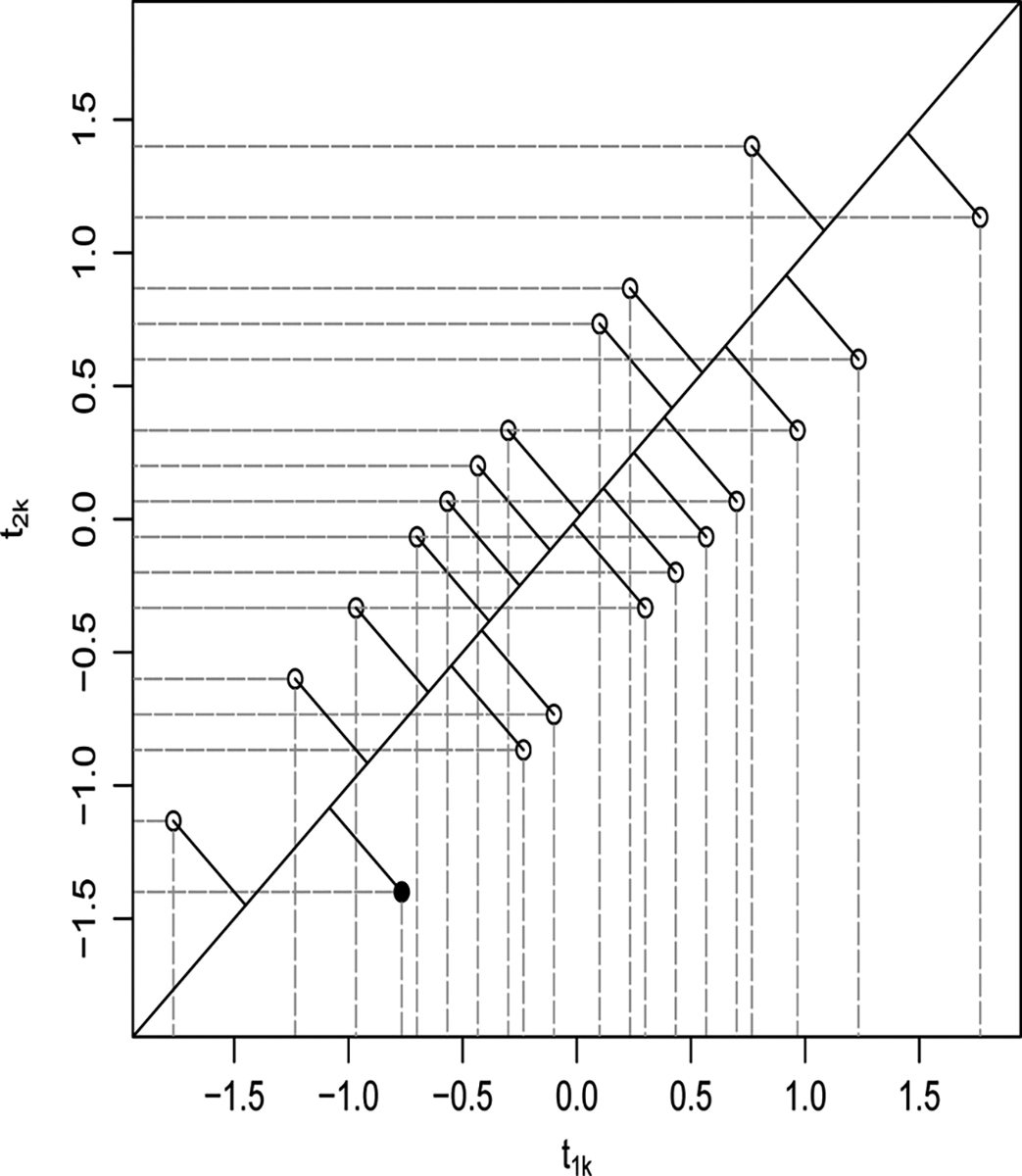
Geometric representation of permutation tests for the data of section 3.1, where everyone provides one measurement except the last person in group 0 who gives 2. Each (x, y) dot corresponds to the pair of test statistics for one of the 20 possible permutations. The x-value (y-value) is based on the first (second) measurement from this last person, the permutation distribution is the horizontal (vertical) projection, and the one-sided p value is 4/20 (1/20). Exhaustive WCR permutation is equivalent to projecting the pair of test statistics onto the 45-degree line. Here, the WCR permutation one-sided p value is 2/20.

Under the null hypothesis that all permutations of Z are equally likely, all two-dimensional points in Fig. 1 are equally likely. We can thus define a rejection region by some shape in two-dimensional space other than the vertical or horizontal lines. A natural test is to take the average of the two test statistics. This test is proportional to the projection of each point onto the 45° line as shown in Fig. 1. The p values are determined by the number of projected support points that are more extreme than the projected test statistic. We see that the lower p value based on this maneuver is p_ℓ = 2/20.

With standard permutation tests, inference is unaffected by any monotone transformation of the test statistic. However, with WCR permutation, this is not the case. Suppose that instead of using the usual test statistic, say t, we used log(t). With WCR permutation OP we would average either t or log(t) and the p values could differ. To ensure that inference is unaffected by monotone transformations of the test statistic one can use ranks. Specifically, let R_jk be the rank of t_jk among t_j1, . . . , t_jb. For each resample we replace the t_jks with these associated ranks. A “rank” WCR permutation p value rank is the the percentile of ${\overline{R}}_{\cdot 0}$ with respect to the empirical distribution of ${\overline{R}}_{\cdot 1},\cdots ,{\overline{R}}_{\cdot b}$.

WCR permutation cannot be applied to permutation tests where the permutation set π₁, . . . , π_b depends on j_j. If this happens then we cannot line up the columns of the matrix of Table 2 correctly. For example, in Fisher’s exact test, we condition on the marginal totals, and if these change with different resamples we cannot apply the procedure. Another example where the permutation set can depend on π is when Z changes within a cluster. An example is a crossover study with Z = (0, 1) or (1, 0) denoting the treatment assignment sequence over the two periods for each person (cluster). Here, one might have an WC resample where only Zs = 0 are selected and a test statistic could not even be calculated.

Since WCRP is a permutation test, it is formally testing the strong null hypothesis that z is a meaningless label. This strong null is a composite that the distribution of cluster sizes and the joint distribution of outcomes given a cluster size are both free of z. In symbols, we test

$$H_0:G(m\mid z)=G(m)\cap F_m\left(x_1,\dots ,x_m\mid z\right)=F_m\left(x_1,\dots ,x_m\right)\text{for}\text{all}m$$

where G( ) is the distribution function of the cluster sizes and F_m( ) is the joint distribution X₁, . . . , X_m. Note that this does allow for informative cluster sizes as F_m( ) can depend on m.

3.2. Example: Permutation t-Test

In some simple cases, we can calculate the final row of Table 2 directly. Consider the two-sample t-test setting where Z_i = 0(1) identifies the control (treatment) group, and person i gives clustered outcomes X_i1, . . . , X_im(i). One can show that exhaustive WCR permutation corresponds to taking the sample average for each person and using these averages in a permutation t-test. That is, the averaged test statistic is

$${\overline{t}}_{\cdot 0}=\frac{{\sum }_{i=1}^n{Z}_i{\overline{X}}_i}{{\sum }_{i=1}^n{Z}_i}-\frac{{\sum }_{i=1}^n\left(1-Z_i\right){\overline{X}}_i}{{\sum }_{i=1}^n\left(1-Z_i\right)}$$ (1)

where ${\overline{X}}_i$ is the within-cluster mean. The b support points of the permutation distribution are

$${\overline{t}}_{\cdot k}=\frac{{\sum }_{i=1}^n{Z}_i\left({\mathit{\pi }}_k\right){\overline{X}}_i}{{\sum }_{i=1}^n{Z}_i\left({\mathit{\pi }}_k\right)}-\frac{{\sum }_{i=1}^n\left\{1-Z_i\left({\mathit{\pi }}_k\right)\right\}{\overline{X}}_i}{{\sum }_{i=1}^n\left\{1-Z_i\left({\mathit{\pi }}_k\right)\right\}}$$

for k = 1, . . . , b, where Z_i(π_k) is the ith element of Z(π_k). Note that this does allow for informative cluster sizes as F_m( ) can depend on m.

3.3. Example: Linear Permutation Tests

Suppose the test statistic for WC resample j can be written as

$$t\{X(\mathit{j}),\mathit{Z}\}=\sum _{i=1}^n{Z}_i{w}_{\mathit{X}}\left\{X_i(\mathit{j})\right\}$$

where w_X( ) is a function that may depend on the entire vector X and possibly other covariates, but cannot depend on Z_i. Then for permutation k we can write

$$\begin{gathered} {\overline{t}}_{\cdot k}=\sum _{i=1}^n{Z}_i\left({\mathit{\pi }}_k\right)\frac{1}{m}\sum _{j=1}^m{w}_X\left\{X_i\left({\mathit{j}}_j\right)\right\} \\ =\sum _{i=1}^n{Z}_i\left({\mathit{\pi }}_k\right)\frac{1}{{\prod }_{\ell =1}^n{m}_{\ell }}\sum _{{\ell }_1=1}^{m_1}\cdots \sum _{{\ell }_n=1}^{m_n}{w}_X\left(X_{i{\ell }_i}\right) \\ =\sum _{i=1}^n{Z}_i\left({\mathit{\pi }}_k\right)\frac{{\prod }_{h\ne i}{m}_h}{{\prod }_{\ell =1}^n{m}_{\ell }}\sum _{{\ell }_i=1}^{m_i}{w}_X\left(X_{i{\ell }_i}\right) \\ =\sum _{i=1}^n{Z}_i\left({\mathit{\pi }}_k\right)\frac{1}{m_i}\sum _{\ell =1}^{m_i}{w}_X\left(X_{i\ell }\right)=\sum _{i=1}^n{Z}_i\left({\mathit{\pi }}_k\right){\overline{w}}_i \end{gathered}$$

This form covers many tests. The permutation t-test has ${\overline{w}}_i={\overline{X}}_i$. An analysis of covariance (ANCOVA) permutation test statistic can be fashioned based on the model

$$X_{ij}={\beta }_0+{\beta }_1{W}_i+\mathrm{\Delta }{Z}_i+{ϵ}_{ij}$$

where ϵ_ij are mean 0 random variables free of Z_i. We then obtain

$${\overline{w}}_i=\frac{\left({\overline{X}}_i-\overline{X}\right)-\left(\overline{W}-W_i\right){\widehat{\beta }}_1(\overline{X})}{n}$$

where ${\widehat{\beta }}_1(\overline{X})$ is the slope of the regression of ${\overline{X}}_i$ on W_i and $\overline{X}={\sum }_i{\overline{X}}_i/n$. The Wilcoxon rank sum test has ${\overline{w}}_i={\overline{R}}_i(\mathit{X})=m^{-1}{\sum }_{i=1}^{m}R\left\{X_i\left({\mathit{j}}_j\right)\right\}$, where R{X_i(j_i)} is the rank of X_i(j_j) among X₁(j_j), . . . , X_n(j_j). Additionally, the distribution permutation tests of Fay and Shih (1998) have ${\overline{w}}_i=n^{-1}{\sum }_{h=1}^n\varphi ({\widehat{F}}_i,{\widehat{F}}_h)$, where ϕ( ) is some function and ${\widehat{F}}_i$ is the empirical distribution function for the responses $X_{i1},\dots ,X_{i{m}_i}$ of cluster i.

4. MONTE CARLO WCR PERMUTATION

4.1. Basic Setup

In many settings, b and m will be too large for exhaustive WCR permutation to be feasible and we must approximate the exact p value by Monte Carlo methods. In this section we discuss how to choose the number of randomly selected Monte Carlo resamples and permutations so that the resultant p value is close to the exhaustive WCR permutation p value.

Let $y_k=I\left({\overline{t}}_{\cdot k}-{\overline{t}}_{\cdot 0}\ge 0\right)$, where k = 1, . . . , b, so that $\overline{y}=p_u$ is the exhaustive WCRP upper p value. To approximate the permutation distribution, we randomly draw a large number, say B, of permutations. Denote the associated indicator functions by $y_K=I\left({\overline{t}}_{\cdot K}-{\overline{t}}_{\cdot 0}\ge 0\right)$, where upper case K = 1, . . . , B are the indices of a random (with replacement) sample of the integers 1, . . . , b. Note that these y₁, . . . , y_B terms are iid Bernoullis with probability p_u. By the Central Limit Theorem (CLT) we know that

$$\frac{1}{B}\sum _{K=1}^B{y}_K\approx N\left(p_u,\frac{p_u\left(1-p_u\right)}{B}\right)$$

One could choose B to achieve any desired level of accuracy.

If m = m₁ × · · · × m_n was small, we could calculate ${\overline{t}}_{\cdot K}$ exactly. If m is large, we will need to estimate ${\overline{t}}_{\cdot K}$. Since we only care if ${\overline{t}}_{\cdot K}\ge {\overline{t}}_{\cdot 0}$, the precision of our estimate of ${\overline{t}}_{\cdot K}$ should depend on how far it is from ${\overline{t}}_{\cdot 0}$. Thus we will allow M_K, the number of randomly selected WC resamples for permutation П_K to vary with K. Let J_J be the Jth Monte Carlo draw from the full set of possible resamples, j₁, . . . , j_m. Also let П_K be the Kth Monte Carlo draw from the full set of possible permutations, π₁, . . . , π_b . We write the test statistic associated with the Jth resample and Kth permutation as T_JK = T{X(J_J), Z(M_K)}. We use upper case T, J, J, П, K to emphasize that they are random variables and not fixed constants as for the exhaustive case. For the Kth selected permutation, we estimate y_K by first drawing M_K WC resamples for this permutation, say, ${\mathit{J}}_{K1},\dots ,{\mathit{J}}_{K{M}_K}$. We then form ${\overline{T}}_{\cdot K}=M_K^{-1}{\sum }_{J=1}^{M_K}T\left\{\mathit{X}\left({\mathit{J}}_{KJ}\right),\mathit{Z}\left({\mathbf{\Pi }}_K\right)\right\}$, and also estimate ${\overline{t}}_{\cdot 0}$ for these same resamples, ${\overline{T}}_{.0}=M_K^{-1}{\sum }_{J=1}^{M_K}T\left\{\mathit{X}\left({\mathit{J}}_{KJ}\right),\mathit{Z}\left({\mathit{\pi }}_0\right)\right\}$. We then form $Y_K=I\left({\overline{T}}_{\cdot K}-{\overline{T}}_{.0}\ge 0\right)$. Note that for each support point we reestimate ${\overline{t}}_{\cdot 0}$. If we used a common estimate for all resamples, then Y₁, . . . , Y_B would not be independent. Although inefficient, using a different ${\overline{T}}_{.0}$ for each response ensures that the Y₁, . . . , Y_B are independent and thus allows easy approximation of $\mathrm{var}(\overline{Y})$.

We define the (upper) Monte Carlo WCRP permutation p value as ${\widehat{p}}_u=B^{-1}{\sum }_{K=1}^B{Y}_K$. In practice, we will often use the asymptotically (on B) equivalent form ${\tilde{p}}_u=\left(1+\sum Y_K\right)/(B+1)$ because it bounds the p value away from zero and ensures proper size (Fay and Follmann, 2002). We want to select each M_K so that each Y_K has a high probability of equaling y_K.

Note that for a fixed K we can think of ${\overline{T}}_{.K}$ as a sample mean based on M_K random draws from the column of Table 2 where π = П_K. That is, from the discrete distribution with support points t_1K, . . . , t_mK. This also applies to ${\overline{T}}_{.0}$. Without loss of generality, let П_K = π_k. By the CLT, as M_K → ∞, ${\overline{T}}_{.K}-{\overline{T}}_{\cdot 0}$ is approximately normal with mean ${\overline{t}}_{\cdot k}-{\overline{t}}_{\cdot 0}$ and variance ${\sigma }_{k0}^2/M_K$, where ${\sigma }_{k0}^2={\sum }_{j=1}^m{\left\{t_{jk}-t_{j0}-\left({\overline{t}}_{\cdot k}-{\overline{t}}_{\cdot 0}\right)\right\}}^2/m$.

For each K we only need to know if ${\overline{t}}_{\cdot K}-{\overline{t}}_{\cdot 0}$ is positive or negative. To achieve this with high probability, we propose the 6-tens algorithm, an ad hoc procedure that chooses M_K so that

$$\left|Z_K\right|\equiv \left|\frac{{\overline{T}}_{\cdot K}-{\overline{T}}_{\cdot 0}}{\sqrt{{\widehat{\sigma }}_{K0}^2/M_K}}\right|$$

is large, and thus the sign of ${\overline{T}}_{\cdot K}-{\overline{T}}_{\cdot 0}$ equals that of ${\overline{t}}_{\cdot K}-{\overline{t}}_{\cdot 0}$ with high probability.

4.2. 6-Tens Algorithm

1. Set M_K = 10 for K = 1, . . . , B. For each of the B selected permutations П₁, . . . , П_B, randomly draw 10 resamples, say J_K1, . . . , J_K10, and calculate

   $$D_{K\ell }=T\left\{\mathit{X}\left({\mathit{J}}_{K\ell }\right),\mathit{Z}\left({\mathbf{\Pi }}_K\right)\right\}-T\left\{\mathbf{X}\left({\mathit{J}}_{K\ell }\right),\mathit{Z}\left({\mathbf{\Pi }}_0\right)\right\}$$

   for ℓ = 1, . . . , 10. Calculate the mean and sample variance of the Ds, say ${\overline{D}}_K$ and $S_{K0}^2$, and form

   $$Z_K=\frac{{\overline{D}}_K}{\sqrt{S_{K0}^2/10}}$$

   Let ${𝒦}_6$ be the set of Ks for which |Z_K| < 6.
2. For each $K\in {𝒦}_6$ set M_K = M_K × 10, randomly generate M_K differences D_Kℓ, and form

   $$Z_K=\frac{{\overline{D}}_K}{\sqrt{S_{K0}^2/M_K}}$$

   Again let ${𝒦}_6$ be the set of Ks for which |Z_K| < 6.

3. Repeat step 2 until either ${𝒦}_6$ is empty, or M_K > M_max, some prespecified maximum value.

4. Let Y_K = I(Z_K > 0), where Z_K is the final value from step 3, and estimate the p value as ${\tilde{p}}_u={(B+1)}^{-1}(1+{\sum }_{K=1}^B{Y}_K)$.

One can show that the expected Monte Carlo p value does not equal the exact p value or $E[\overline{Y}]\ne \overline{y}$, so bias can be a problem in principle. With the 6-tens algorithm we try to essentially eliminate bias by making each Y_K a very good estimate of y_K. In the Appendix the bias of $\overline{Y}$ is explored in more detail, along with a more formal justification of the 6-tens algorithm.

4.3. Evaluation of the 6-Tens Algorithm

To empirically evaluate the 6-tens algorithm, we conducted a simple simulation. We assumed that the true support points ${\overline{t}}_{\cdot k}$ followed a normal(0,τ²) distribution and that the variance of $T_{jk}\mid {\overline{t}}_{\cdot k}$ was σ². We fixed ${\overline{t}}_{\cdot 0}>0$ so the WCRP upper p value was $\mathrm{\Phi }\left(-{\overline{t}}_0/\tau \right)$. We pretended that σ² was known and did not estimate it. We randomly selected B = 1000 permutations (true support points) and calculated $\overline{y}$, the “true” p value for that choice of permutations/support points. Note that $\overline{y}\approx \mathrm{\Phi }\left(-{\overline{t}}_0/\tau \right)$. This approximation becomes exact as B → ∞. We fixed this set of support points/permutations and then repeated the 6-tens algorithm 10,000 times. For each of these 10,000 repeats, we calculated $\overline{Y}$ and $\widehat{\mathrm{var}}[\overline{Y}]$. The objective was to see whether the 6-tens algorithm worked well in terms of bias, mean squared error (MSE), and accuracy of the variance approximation (10), for a specific set of permutations.

Table 3 shows an unsurprising decrease in bias as max M_K increases. Importantly, the average estimated variance appears quite close to the actual sample variance, suggesting the approximation of (10) will be useful in setting sample size. While the scenarios here are limited, a maximum of 10, 000 seems to be a reasonable choice for the 6-tens algorithm.

Table 3.

Simulated performance of the 6-tens algorithm

σ	${\overline{t}}_{\cdot 0}$	max(MK)	$\overline{y}$	%|ZK|s < 6	bias	MSE	$\overline{\widehat{\mathrm{var}}[\overline{Y}]}$	$S^2(\overline{Y})$
1	1	100	.144	.415	4.2 × 10−3	3.5 × 10−5	1.9 × 10−5	1.8 × 10−5
1	1	10000	.161	.040	−5.0 × 10−5	1.9 × 10−6	1.7 × 10−6	1.6 × 10−6
1	1	1000000	.156	.003	−2.6 × 10−5	2.6 × 10−8	6.2 × 10−8	2.5 × 10−8
1	2	100	.020	.133	2.5 × 10−3	1.1 × 10−5	4.6 × 10−6	4.8 × 10−6
1	2	10000	.019	.006	6.6 × 10−4	9.3 × 10−7	4.0 × 10−7	4.9 × 10−7
1	2	1000000	.017	.000	0	0	2.6 × 10−14	0
.1	1	100	.174	.040	−1.5 × 10−3	3.4 × 10−6	1.5 × 10−6	1.2 × 10−6
.1	1	10000	.175	.004	−1.7 × 10−6	9.3 × 10−9	5.2 × 10−8	9.3 × 10−9
.1	1	1000000	.158	.0	0	0	4.7 × 10−15	0
.1	2	100	.022	.009	−1.9 × 10−4	3.8 × 10−7	3.7 × 10−7	3.4 × 10−7
.1	2	10000	.023	0	0	0	1.1 × 10−15	1.2 × 10−35
.1	2	1000000	.020	0	0	0	1.8 × 10−15	0

Note. Each line represents a summary of 10,000 estimates ($\overline{y}$) of a single WCR permutation p value $\overline{y}$ based on a specific set of 1000 permutations (support points). Bias is the average of the 10,000 differences $\overline{Y}-\overline{y}$. MSE is the average of the 10,000 squared differences ${(\overline{Y}-\overline{y})}^2$.$S^2(\overline{Y})$ is the sample variance of the $\overline{Y}\text{s}$.

5. A MORE GENERAL FORM OF THE TEST

Although we have spoken only about conditional permutation tests, we can generalize to other tests that are permutation-like. In this section, Z denotes a random vector from a distribution f_Z(z) where z is a realization of this variable. First we write the permutation tests in a form that will be easily generalized. Let $\overline{t}(\mathit{z})=m^{-1}{\sum }_{j=1}^{m}t\left\{\mathit{X}\left({\mathit{j}}_j\right),\mathit{z}\right\}$, so that ${\overline{t}}_{\cdot k}=\overline{t}\left\{\mathit{z}\left({\mathit{\pi }}_k\right)\right\}$. Then we generalize the lower WCRP p value by writing it as

$$E_{\mathit{Z}}\left[I\left\{\overline{t}(\mathit{Z})\le \overline{t}\left(z_0\right)\right\}\right]$$ (2)

where E_Z represents expectation over the n-dimensional random vector Z, and z₀ is the observed value of z. In the usual setting, the distribution of Z has b equally likely support points, and f_Z is the permutation distribution on Z, such that

$$f_{\mathit{Z}}(\mathit{z})=\{\begin{array}{ll}\frac{1}{b}\hfill & \text{if}\mathit{z}={\mathit{z}}_0\left({\mathit{\pi }}_k\right)\text{for}k=1,\dots ,b\hfill \\ 0\hfill & \text{otherwise}\hfill \end{array}$$

In that case we condition on the observed value Z = z₀ and consider permutations of that observed value. We can generalize to unconditional tests by allowing the null hypothesis distribution of Z to not be conditional on z₀. For example, one could let f_Z be an n-dimensional continuous distribution with an infinite number of support points. In section 7.3 we give an example where z₀ is an n-dimensional zero vector, and f_Z is continuous with

$$f_{\mathit{Z}}(\mathit{Z})=\{\begin{array}{ll}\frac{1}{2\pi n}\hfill & \text{if}{Z}_i\in [0,2\pi ]\text{for}\text{all}i\in \{1,\dots ,n\}\hfill \\ 0\hfill & \text{otherwise}\hfill \end{array}$$

where π ≈ 3.14 . . . is the irrational number, not a permutation. The lower p value is still represented by Eq. (2).

6. SIMULATION

To evaluate the performance of different tests for clustered data, we conducted a small simulation for the two-sample setting. We generated data under a normal mixture model: X_ij = μZ_i + b_i + ϵ_ij, where i = 1, . . . , 2n indexes clusters, j = 1, . . . , m_i indexes observations within clusters, Z_i = 0, 1 is the treatment group indicator for cluster i, m_Z the cluster sizes for group Z = 0, 1, and there are n clusters per group. We generated $b_i~N\left(0,{\sigma }_b^2\right)$ and ${ϵ}_{ij}~N\left(0,{\sigma }_e^2\right)$ with all b’s and ϵ’s independent. We considered 36 different situations as follows:

• $\left({\sigma }_b^2,{\sigma }_e^2\right)$ = (0, 1), (1, 1), and (1, 0). These correspond to within-cluster correlations of 0, 0.5, and 1.

• μ = 0 or a where a was chosen to so that EOP had approximately 80% power.

• Three types of cluster sizes were considered: rectangular: m_i = 5, triangular: m_i = i, and informative: m_i = 1 × I(b_i ≤ 0) + 10 × I(b_i > 0)

• Number of clusters per group = 5 or 15.

We evaluated three tests, single WCR permutation (SWCRP), exhaustive WCR permutation (EWCRP), and the Wilcoxon rank sum test of Datta and Satten (2005) (DS). For SWCRP the test statistic is the difference means of the first observation in each cluster;

$$T_0^S=\frac{{\sum }_{i=1}^{2n}{Z}_i{X}_{i1}}{{\sum }_{i=1}^{2n}{Z}_i}-\frac{{\sum }_{i=1}^{2n}\left(1-Z_i\right)X_{i1}}{{\sum }_{i=1}^{2n}\left(1-Z_i\right)}$$

while for EWCRP the test statistic is the difference in cluster means,

$$T_0^E=\frac{{\sum }_{i=1}^{2n}{Z}_i{\overline{X}}_i}{{\sum }_{i=1}^{2n}{Z}_i}-\frac{{\sum }_{i=1}^{2n}\left(1-Z_i\right){\overline{X}}_i}{{\sum }_{i=1}^{2n}\left(1-Z_i\right)}$$

The test of Datta and Satten is a WCR version of the Wilcoxon test and is based on

$$W_J^{*}=\frac{1}{M}\sum _{i=1}^n{Z}_i\mathrm{Rank}\left(X_{iJ(i)}\right)$$

the sum of the ranks for a randomly selected WCR, J. The test is based on forming $E\left[W_J^{*}\right]$, where the expectation is over J, and then standardizing $E\left[W_{\mathit{J}}^{*}\right]$ and comparing the standardized test statistic to an asymptotically valid standard normal null distribution.

For all permutation-based test statistics, we simulated the permutation distribution by scrambling the Z_is 299 times and rejected the one-sided null at α = .05 if the simulated p value $\{1+{\sum }_{p=1}^{299}I\left(T_p\ge T_0\right)\}/300$ was smaller than .05, where T_p is the pth permuted test statistic. Note that $T_0^E$ exhausts all within-cluster resamples, but uses Monte Carlo approximation for the permutation distribution.

From Table 4, we see that both EWCRP and SWCRP always control the type I error rate, as they must. For Datta and Satten, there is some minor inflation for n = 15 and more substantial inflation with n = 5. This is entirely expected as Datta and Satten’s null distribution is based on an asymptotic argument. Thus, as always, if control of the type I error rate is a major concern, exact methods such as EWCRP have appeal. For n = 15, the power of Datta and Satten’s test is quite similar to EWCRP under rectangular and triangular data structure for the m_is. Under an informative cluster size, EWCRP is more powerful for ρ = .5 and 1. For n = 5, the EWCRP has similar or somewhat less power than Datta and Satten for the rectangular and triangular data structures—presumably a consequence of the coarseness of the permutation distribution for small n, and the modest type I error rate inflation of Datta and Satten. For the informative cluster size setting, the EWCRP has better power for ρ = .5 and 1.

Table 4.

Proportion of rejections for different tests of equality of two distributions

mis	μ	ρ	SWCRP	EWCRP	DS	n/2
Rectangular	0	0	0.0510	0.0505	0.0538	15
Rectangular	0	.5	0.0504	0.0495	0.0529	15
Rectangular	0	1	0.0519	0.0519	0.0545	15
Rectangular	a	0	0.3080	0.8180	0.8164	15
Rectangular	a	.5	0.5466	0.7341	0.7451	15
Rectangular	a	1	0.7299	0.7299	0.7260	15
Triangular	0	0	0.0504	0.0508	0.0540	15
Triangular	0	.5	0.0498	0.0503	0.0532	15
Triangular	0	1	0.0505	0.0505	0.0526	15
Triangular	a	0	0.3045	0.7874	0.7719	15
Triangular	a	.5	0.5456	0.7278	0.7338	15
Triangular	a	1	0.7272	0.7272	0.7165	15
Informative	0	0	0.0503	0.0503	0.0539	15
Informative	0	.5	0.0501	0.0504	0.0375	15
Informative	0	1	0.0499	0.0499	0.0180	15
Informative	a	0	0.5819	0.8061	0.7924	15
Informative	a	.5	0.6471	0.7438	0.6858	15
Informative	a	1	0.7307	0.7307	0.5751	15
Rectangular	0	0	0.0472	0.0487	0.0615	5
Rectangular	0	.5	0.0486	0.0478	0.0621	5
Rectangular	0	1	0.0478	0.0478	0.0471	5
Rectangular	a	0	0.2736	0.7547	0.7943	5
Rectangular	a	.5	0.6651	0.6651	0.6512	5
Rectangular	a	1	0.4932	0.6723	0.7313	5
Triangular	0	0	0.2744	0.4847	0.5148	5
Triangular	0	.5	0.4900	0.6008	0.6474	5
Triangular	0	1	0.6667	0.6667	0.6797	5
Triangular	a	0	0.0468	0.0463	0.0624	5
Triangular	a	.5	0.0487	0.0465	0.0607	5
Triangular	a	1	0.0480	0.0480	0.0558	5
Informative	0	0	0.0484	0.0483	0.0653	5
Informative	0	.5	0.0471	0.0481	0.0436	5
Informative	0	1	0.0484	0.0484	0.0187	5
Informative	a	0	0.5223	0.7567	0.7518	5
Informative	a	.5	0.5838	0.6813	0.6572	5
Informative	a	1	0.6653	0.6653	0.5437	5

Note. Within clusters, data are multivariate normal with correlation ρ. The mean cluster difference between groups is μ and varies for different scenarios. Cluster sizes and tests are described in the text.

7. EXAMPLES

7.1. Viral Blips and HIV Infection

The introduction of highly active antiretroviral therapy (HAART) has had a profound impact on the treatment of patients with HIV. Potent combinations of drugs can often render the load of virus (VL) circulating in the blood below the limit of detection of common assays, currently 50 copies/ml. However, even during periods of sustained viral suppression, sometimes “blips” occur—occasions when the amount of virus is above the limit of detection. The meaning of such blips is controversial and under investigation (Di Mascio et al., 2004). Part of their investigation focused on whether the occurrence of blips was associated with a change in the number of CD4 cells, cells of the adaptive immune system that both fight and are infected by HIV.

One approach to this problem would be to build a fairly complicated model for the repeated CD4 and VL data. If such a model could be correctly specified it could then be used to draw conclusions about various hypotheses, including the effect of blips on CD4 and CD8 cells. A different approach is to test specific hypotheses using simple statistics that are easily described and understood by a medical audience.

If the increase in virions during a blip impairs the recovery of CD4 cells, the relative change in CD4 counts on two successive visits starting with a nonblip and ending with a blip, say, R₀₁ = (CD4_i − CD4_i−1)/CD4_i−1, should tend to be lower than the analogous relative change ending in a nonblip, say, R₀₀. If each patient provided a single pair R₀₁, R₀₀, then one could form D = R₀₁ − R₀₀. The associated D₁, . . . , D_n could be the data for a paired difference t-test. However, patients generally have sustained periods of viral suppression and thus many R₀₀s and several R₀₁s. In our dataset there are 44 patients with acute HIV infection with both 00 and 01 couples. The total number of couples was 1094 and the mean (SD) number of couples per person was 24.5 (9.9). The mean (SD) number of 01 couples was 2.5 (1.9).

Here exhaustive WCR permutation corresponds to taking the sample average for each patient and using these averages in a permutation test. Thus we form $D={\overline{R}}_{01}-{\overline{R}}_{00}$ for each patient and then take the average of these average differences to form our test statistic:

$${\overline{t}}_{\cdot k}=\sum _{i=1}^n\frac{Z_i\left({\mathit{\pi }}_k\right)D_i}{n}$$

where Z_i = ±1 and Z(π₁), . . . , Z(π_b) enumerates the b = 2ⁿ possible signs of an n-vector. There were 44 patients who had both 00 and 01 couples during acute infection. The exact upper p value here is .1793, and took about 30 s to calculate on a desktop computer.

A random effects model could also be fit to these data, where

$$R_{ij}=b_i+\mathrm{\Delta }{Z}_{ij}+{\mathit{ϵ}}_{ij}$$

where b_i, ϵ_ij are independent normals with mean zero and variances τ² and σ², respectively, R_ij is the relative change in CD4 count for patient i for the jth couple, and Z_ij is the indicator for whether this couple started with a blip in viremia. This approach makes parametric assumptions and the p value for testing Δ = 0 is .14.

7.2. Heart Function in HIV-Infected Children

A retrospective study of 133 HIV-infected children was conducted at the National Institutes of Health to assess the contributions of progressive HIV disease (as measured by CD4 counts and percentages), vertical transmission, and azidothymidine (AZT) on cardiac function (Domanski et al., 1995). Cardiac function was measured by the fractional shortening of the left ventricle, which is essentially the fractional decrease in volume during a heartbeat, and larger values are desirable. Table 5 provides some descriptive statistics for the variables of interest, including averages of all the measurements and averages of each patient’s values.

Table 5.

Descriptive statistics for the study of factors on the fractional shortening of the left ventricle in children with AIDS (Domanski et al., 1995)

Variable	Σmi = 486 measurements			Mean of n cluster averages
	Mean	Minimum	Maximum
Fractional shortening	0.34	0.05	0.59	0.34
CD4 cells	455.6	0	3421	544.8
Percent CD4 cells	16.1	0	63	18.1
I (AZT)	0.53	0	1	0.53
I (vertical)	0.51	0	1	0.60
Age	7.2	.33	17.11	6.4

Of primary interest was the effect of the covariates on fractional shortening:

$$E\left[{\text{FS}}_{ij}\right]={\beta }_0+{\text{age}}_{ij}{\beta }_1+{\text{CD}}_{ij}{\beta }_2+\%{\text{CD}}_{ij}{\beta }_3+I{(\text{AZT})}_{ij}{\beta }_4+I{(\text{vertical})}_i\mathrm{\Delta }$$ (3)

where i = 1, . . . , n = 133 and j = 1, . . . , m_i. Thus i, j is the jth visit of the ith patient and age_ij, CD4_ij are the age and CD4 count, % CD4_ij is the percentage of CD4 cells among the white blood cells, I(AZT)_ij is 1 if on AZT, and I(vertical)_i is 1 if infected by the mother.

For regression, there are different approaches to permutation analysis (see Edgington, 1995; Kennedy and Cade, 1996; Manly, 1997). We use “permutation under the reduced model” (Freedman and Lane, 1983) as recommended by Anderson and Legendre (1999) to evaluate the effect of I(vertical). Permutation methods can be more powerful than the normal t-test approach if the errors are non-normal (Anderson and Legendre, 1999). Using an obvious notation, we write the regression model of Eq. (3), for a single resample J of n independent data points as

$$X_{J(i)}={\mathit{W}}_{J(i)}^{\prime }\mathit{\beta }+Z_{J(i)}\mathrm{\Delta }+{\mathit{ϵ}}_{J(i)}$$ (4)

for i = 1, . . . , n, where Z is I(vertical), and ϵ_J(i) is an error term. As a test statistic, we use the usual t-statistic for testing Δ = 0 based on least-squares regression of X on W, Z:

$$T\left\{\mathit{X}(\mathit{J}),\mathit{Z}\left({\mathbf{\Pi }}_0\right)\right\}=\frac{\widehat{\mathrm{\Delta }}\left(\mathit{J},{\mathbf{\Pi }}_0\right)}{\sqrt{\widehat{\mathrm{var}}\{\widehat{\mathrm{\Delta }}\left(\mathit{J},{\mathbf{\Pi }}_0\right)\}}}$$ (5)

To obtain a permutation distribution for this test, we randomly select a permutation П and perform an initial regression without Z:

$$X_{J(i)}={\mathit{W}}_{J(i)}^{\prime }{\mathit{\beta }}^r+{\mathit{ϵ}}_{J(i)}^r$$ (6)

The permuted residuals, ${\widehat{\mathit{ϵ}}}_{J(\mathrm{\Pi }(i))}^r$ are added to the predicted Xs from this regression to form X*

$$X_{J(i)}^{*}={\mathit{W}}_{J(i)}^{\prime }{\widehat{\mathit{\beta }}}^r+{\widehat{\mathit{ϵ}}}_{J(\mathrm{\Pi }(i))}^r$$ (7)

where П(i) is the ith element of the permutation vector П. Then the newly created X* is regressed on the original W, Z:

$$X_{J(i)}^{*}={\mathit{W}}_{J(i)}^{\prime }\mathit{\beta }+Z_{J(i)}\mathrm{\Delta }+{ϵ}_{J(i)}$$ (8)

and based on this regression, the usual t-statistic for testing Δ = 0 is formed: T{X(J), Z(П)} from Eq. (5). For Monte Carlo WCR with the 6-tens algorithm, the preceding steps (6), (7), and (8) are repeated M_K times for both П_K and П₀. One can show that the T{X(J), Z(П₀)} as defined in Eq. (5) based on Eq. (4) also obtains from the procedure defined by Eqs. (6), (7), and (8) with П = П₀.

Using the preceding methods we tested the relationship between fractional shortening and vertical transmission while controlling for the effects of the four confounders. We used the 6-tens algorithms with B = 1999 and M_Max = 10⁵ and obtained a lower p value of p = .4745 with standard error of 0.011, where 99.8% of the variance estimate is due to the second term of (10):$\overline{Y}(1-\overline{Y})/B$. This calculation took approximately 13 h on a PC.

One can also analyze these data using GEE (Liang and Zeger, 1986). We postulate a working independence correlation matrix and calculate a Wald statistic for Δ of −.32, which corresponds to a p value of .37. This method uses an asymptotic null distribution in contrast to WCRP, which can be liberal if the number of clusters is small or the covariates are not balanced (Fay and Graubard, 2001).

7.3. Correlated Angular Measurements

Follmann and Proschan (1999) discuss the problem of testing uniformity with correlated angular data. Of interest was whether times of seizures have a circadian pattern, or whether they are uniformly distributed on the 24-hour clock. Data from 12 patients were provided; one patient had one seizure, while another had 36 with a cluster of seizures a little before midnight.

Follmann and Proschan (1999) introduced a definition of uniformity called rotation invariance and provided several tests for rotation invariance that explicitly allowed for arbitrary clustering/correlation of angles within a cluster. Developing new methodology can be time-consuming, and it is also nice to have simple tools to attack complicated problems. The basic data here is the long vector

$$\mathit{X}=\left(X_{11},\dots ,X_{1m_1},X_{21},\dots ,X_{2m_2},\dots ,X_{n1},\dots ,X_{n{m}_n}\right),$$

where X_ij is the jth seizure time on the 24-hour clock (in radians) for individual i. A seizure at 6:00 a.m. = 0 radians and a seizure at noon = 3π/2 radians.

A standard test of uniformity for angular data is the Rayleigh test. For a single “resample” J, the Rayleigh test statistic is

$$T\{\mathit{X}(\mathit{J})\}={\left[\frac{\sum \cos \left\{X_i(\mathit{J})\right\}}{n}\right]}^2+{\left[\frac{\sum \sin \left\{X_i(\mathit{J})\right\}}{n}\right]}^2$$

If T{X(J)} is close to 0, the angles are scattered, while if T{X(J)} is close to 1, the angles have a definite preferred direction. Mardia (1972) provides the exact null distribution of R and argues that for large n, 2nT{X(J)}² is approximately chi-square with 2 degrees of freedom. Though unnecessary here since the null distribution is known (Mardia, 1972), one could simulate the null distribution of T{X(J)} by forming

$$T\{\mathit{X}(\mathit{J}),\mathit{Z}\}={\left[\frac{\sum \cos \left\{X_i(\mathit{J})+Z_i\right\}}{n}\right]}^2+{\left[\frac{\sum \sin \left\{X_i(\mathit{J})+Z_i\right\}}{n}\right]}^2$$

where Z = (Z₁, . . . , Z_n), and the Z_i are independent and uniform (0, 2π). One would generate many such Zs and the associated Ts would comprise a simulated null reference distribution.

We apply the idea of Monte Carlo WCR permutation using the general setup described in Section 5. We randomly generate B n-vectors, Z₁, . . . , Z_B, where Z_K = (Z_K1, . . . , Z_Kn) and each Z_Ki is uniform (0, 2π). For each Z_K, we form

$$D_{K\ell }=\sum _{J=1}^{M_K}T\left\{\mathit{X}\left({\mathit{J}}_J\right),{\mathit{Z}}_K\right\}-T\left\{\mathit{X}\left({\mathit{J}}_J\right),\mathbf{0}\right\}$$

We applied the 6-tens algorithm with B = 1999 and M_Max = 10⁵ and obtained an upper p value of 1528/2000. The estimate of the standard deviation, from Eq. (10), of that p value is .011, with 98.7% of the variance estimate due to the second term of Eq. (10):$\overline{Y}(1-\overline{Y})/B$. This calculation took approximately 10 h on a personal computer (PC). The tests of Follmann and Proschan for the null hypothesis of rotation invariance all provide p values greater than .40.

8. SUMMARY

This paper has introduced a general method for obtaining exact permutation results in the presence of arbitrary within cluster correlation by using within cluster resampling. A fixed set of permutations is selected, and then for each cluster a single outcome is randomly selected and a test statistic calculated for each permutation. The procedure of drawing a single outcome from each cluster is repeated many times, and the test statistics for each specific permutation are averaged over all WC resamples. These averaged test statistics are used as the null reference distribution for the averaged test statistic. In practice, Monte Carlo methods to approximate the permutation distribution may be required. An algorithm is proposed where computational effort is focused to determine whether the support points of the null distribution fall to the left or right of the test statistic, thus ensuring an accurate approximate p value. Different examples are used to illustrate the broad application of WCR permutation. WCR permutation is a handy and simple way to apply permutation methods when within-cluster correlation is a nuisance.

APPENDIX: BIAS OF $\overline{\mathit{Y}}$

It is instructive to explore how bias becomes a substantial problem if one uses a small number of Monte Carlo resamples. This analysis also demonstrates how the easy approach of doing single resamples and averaging the p values over many resamples is generally conservative.

For this section, suppose that M_K = M for all K, and define $p(B,M)=\overline{Y}$ as the p value based on B random permutations and M random resamples. For a fixed dataset, p(B, M) is still a random variable dependent on the specific resamples and permutations that were selected. Since E[p(B, M)] is free of B, we use $E\{p(\infty ,M)\}=E(\overline{Y})$ to denote the expected Monte Carlo WCR p value based on M resamples. To see the problem for small samples, consider again the made-up data of section 3.1. Suppose that we set M = 1 but enumerate the 20 permutations. Thus the p value is either 1/20 or 4/20 and both occur with equal probability. Formally we can write

$$E[p(\infty ,1)]=\frac{1}{20}Pr\left(\mathit{J}={\mathit{j}}_1\right)+\frac{4}{20}Pr\left(\mathit{J}={\mathit{j}}_2\right)=5/40$$

which is larger than p(∞, ∞) = 2/20. If we set M = 2, then E[p(∞, 2)] = 9/80, which is still larger than p(∞, ∞). One can show that E[p(∞, M)] is not monotone for this small dataset, and one can produce datasets where $E[p(\infty ,M)]\le p(\infty ,\infty )=\overline{y}$. Thus, the bias can go in either direction.

To get a handle on the form of the bias in large samples, we worked out some asymptotics for the two-group test statistic of Eq. (1). By the CLT, ${\overline{T}}_{\cdot K}\approx N\left({\overline{t}}_{\cdot K},{\sigma }_K^2/M\right)$ where ${\sigma }_K^2={\sum }_{j=1}^m{\left(t_{jK}-{\overline{t}}_{\cdot K}\right)}^2/m$. As n → ∞ the distribution of ${\overline{t}}_{\cdot K}$, based on the difference in means statistic, approaches that of a normal distribution with mean 0 and some variance, say τ², by the permutational CLT (Sen, 1985). One can also show that ${\sigma }_K^2={\sigma }^2$ for the difference in means statistic. Thus, if we knew ${\overline{t}}_{\cdot 0}$ we would have the following approximation for the expected p value based on M WC resamples:

$$E\{p(\infty ,M)\}=E\left\{I\left({\overline{T}}_{\cdot K}-{\overline{t}}_{.0}\right)\right\}\approx 1-\mathrm{\Phi }\left(\frac{{\overline{t}}_{\cdot 0}}{\sqrt{{\tau }^2+{\sigma }^2/M}}\right)$$ (9)

where the second expectation is over K, the random permutation index.

With Eq. (9), we see that the approximate asymptotic bias decreases with M and increases with σ²/τ². To graphically appreciate this point, consider Fig. 2, which is a plot of the exhaustive and Monte Carlo WCR p values for a large dataset assuming normality of the ${\overline{t}}_{\cdot K}\text{s}$, normality of ${\overline{T}}_{\cdot K}\mid {\overline{t}}_{\cdot K}$ and knowledge of ${\overline{t}}_{\cdot 0}$. The area to the right of ${\overline{t}}_{\cdot 0}$ based on the ${\overline{T}}_{\cdot K}\text{s}$ is approximately E{p(∞, M)}, and this is larger than the area to the right of ${\overline{t}}_{\cdot 0}$ based on the ${\overline{t}}_{\cdot K}\text{s}$, which is p(∞, ∞). Thus, the average of single WC resample p values should be larger than the exhaustive WCR p value.

Figure 2.

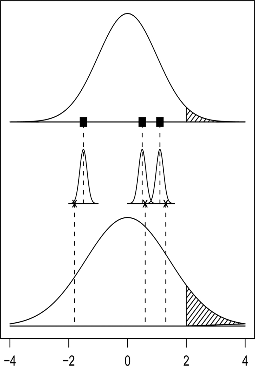
Illustration of the sources of variability in the averaged permutation distribution for the difference in means statistic. The top panel shows the approximate Gaussian (0, τ²) distribution of the ${\overline{t}}_k\text{s}$, i.e., exhaustive WCR permutation distribution. Conditional on ${\overline{t}}_k$, ${\overline{T}}_{\cdot k}$ has an approximate Gaussian $\left({\overline{t}}_k,{\sigma }^2/M\right)$ distribution. Thus unconditionally, the Monte Carlo WCR permutation distribution (bottom panel) is more spread out than the exhaustive permutation distribution. The shaded area of the bottom panel is larger than for the top panel, illustrating that the Monte Carlo p value is likely to be larger than the exhaustive p value.

APPENDIX: JUSTIFICATION OF THE 6-TEN’S ALGORITHM

Note that for the fixed permutations П₁, . . . , П_B, we have Y_K as independent Bernoullis with

$$P\left(Y_K=1\right)=P\left(\frac{{\overline{T}}_{\cdot K}-{\overline{T}}_{\cdot 0}}{\sqrt{{\sigma }_{K0}^2/M_K}}>0\right)\approx \mathrm{\Phi }\left(\frac{{\overline{t}}_{\cdot K}-{\overline{t}}_{\cdot 0}}{\sqrt{{\sigma }_{K0}^2/M_K}}\right)\approx \mathrm{\Phi }\left(Z_K\right)$$

In the preceding, the first approximation is by the CLT and the second one is because we replace the parameters ${\overline{t}}_{\cdot K}$, ${\overline{t}}_{\cdot 0}$, and ${\sigma }_{K0}^2$ with estimates. This approximation works because for each K (except those with ${\overline{t}}_{\cdot K}={\overline{t}}_{\cdot 0}$), |Z_K| → ∞ as M_K → ∞. We thus can approximate the variance of ${\tilde{p}}_u$ for this set of permutations:

$$\widehat{\mathrm{var}}\left(\overline{Y}\mid {\mathbf{\Pi }}_1,\dots ,{\mathbf{\Pi }}_B\right)=\sum _{K=1}^B\frac{\mathrm{\Phi }\left(Z_K\right)\left\{1-\mathrm{\Phi }\left(Z_K\right)\right\}}{B^2}$$

The overall variance estimate for our p value $\overline{Y}$ is

$$\begin{gathered} \mathrm{var}(\overline{Y})=E\left\{\mathrm{var}\left(\overline{Y}\mid {\mathbf{\Pi }}_1,\dots ,{\mathbf{\Pi }}_B\right)\right\}+\mathrm{var}\left\{E\left(\overline{Y}\mid {\mathbf{\Pi }}_1,\dots ,{\mathbf{\Pi }}_B\right)\right\} \\ \approx E\left[\sum _{K=1}^B\frac{\mathrm{\Phi }\left(Z_K\right)\left\{1-\mathrm{\Phi }\left(Z_K\right)\right\}}{B^2}\right]+\mathrm{var}\left(\frac{1}{B}\sum _{K=1}^B{y}_K\right) \\ \approx \sum _{K=1}^B\frac{\mathrm{\Phi }\left(Z_K\right)\left\{1-\mathrm{\Phi }\left(Z_K\right)\right\}}{B^2}+\frac{\overline{Y}(1-\overline{Y})}{B} \end{gathered}$$ (10)

The second line approximation is because we approximate P(Y_K = 1) by Ф(Z_K). The third line approximation is because we replace the expectation of a random variable with a realization of that random variable and we use $\overline{Y}$ to estimate the exhaustive WCR p value $\overline{y}$. Note that with the 6-tens algorithm, most |Z_K|s are large so $\overline{Y}(1-\overline{Y})/B$ is the dominant term of Eq. (10).

REFERENCES

- Anderson M, Legendre P (1999). An empirical comparison of permutation methods for tests of partial regression coefficients in a linear model. Journal of Statistical Computation and Simulation 62:271–303. [Google Scholar]
- Braun T, Feng Z (2001). Optimal permutation tests for the analysis of group randomized trials. Journal of the American Statistical Association 96:1424–1432. [Google Scholar]
- Cai J, Shen Y (2000). Permutation tests for comparing marginal survival functions with clustered failure time data. Statistics in Medicine 19:2963–2973. [DOI] [PubMed] [Google Scholar]
- Datta S, Satten G (2005). Rank tests for clustered data. Journal of the American Statistical Association 100:908–915. [Google Scholar]
- Datta S, Satten G (2008). A signed-rank test for for clustered data. Biometrics Association 64:501–507. [DOI] [PubMed] [Google Scholar]
- Di Mascio M, Markowitz M, Louie M, Hurley A, Hogan C, Simon V, Follmann D, Ho DD, Perelson AS (2004). Dynamics of intermittent viremia during highly active antiretroviral therapy in patients who initiate therapy during chronic versus acute and early human immunodeficiency virus type 1 infection. Journal of Virology 78(19):10566–10573. [DOI] [PMC free article] [PubMed] [Google Scholar]
- Domanski M, Sloas M, Follmann DA, Scallise PP, Tucker EE, Egan D, Pizzo P (1995). Effect of zidovudine and didanosine treatment on cardiac function in human immunodeficiency virus infected children. Journal of Pediatrics 127:137–146. [DOI] [PubMed] [Google Scholar]
- Edgington ES (1995). Randomization Test. 3rd ed. New York: Marcel Dekker. [Google Scholar]
- Fay MP, Follmann D (2002). Designing Monte Carlo implementations of permutation or bootstrap hypothesis tests. American Statistician 56:63–70. [Google Scholar]
- Fay MP, Graubard BI (2001). Small-sample adjustments for Wald-type tests using sandwich estimators. Biometrics 57(4):1198–1206. [DOI] [PubMed] [Google Scholar]
- Fay MP, Shih JH (1998). Permutation tests using estimated distribution functions. Journal of the American Statistical Association 93:387–396. [Google Scholar]
- Follmann DA, Proschan MA, Leifer E (2003). Multiple outputation: Inference for complex multivariate data by averaging analyses from univariate data. Biometrics 59:420–429. [DOI] [PubMed] [Google Scholar]
- Follmann DA, Proschan MA (1999). A simple permutation-type method for testing circular uniformity with correlated angular measurements. Biometrics 55:782–791. [DOI] [PubMed] [Google Scholar]
- Freedman D, Lane D (1983). A nonstochastic interpretation of reported significance levels. Journal of Business and Economic Statistics 1:292–298. [Google Scholar]
- Gail M, Mark S, Carroll R, Green S, Pee D (1996). On design considerations and randomization-based inference for community intervention trials. Statistics in Medicine 15:1069–1092. [DOI] [PubMed] [Google Scholar]
- Hoffman EB, Sen PK, Weinberg C (2001). Within-cluster resampling. Biometrika 88:1121–1134. [Google Scholar]
- Kennedy PE, Cade BS (1996). Randomization tests for multiple regression. Communications in Statistics: Simulation and Computation 25:923–936. [Google Scholar]
- Liang K-Y, Zeger S (1986). Longitudinal analysis using generalized linear models. Biometrika 73:13–22. [Google Scholar]
- Manly BFJ (1997). Randomization and Monte Carlo Methods in Biology. London: Chapman and Hall. [Google Scholar]
- Mardia KV (1972). Statistics of Directional Data. New York: Academic Press. [Google Scholar]
- Rosner B, Glynn R, Lee M-L (2003). Incorporation of clustering effects for the Wilcoxon Rank Sum Test: A large-sample approach. Biometrics 59:1089–1098. [DOI] [PubMed] [Google Scholar]
- Sen PK (1985). Permutational central limit theorem. In: Kotz Balakrishnan, Read Vidakovic, Johnson, eds. Encyclopedia of Statistical Sciences. 2nd ed. pp. 6069–6073. [Google Scholar]
- Williamson J, Datta S, Satten G (2003). Marginal analyses of clustered data when cluster size is informative. Biometrics 59:36–42. [DOI] [PubMed] [Google Scholar]