Sports analytics in the NFL: classifying the winner of the superbowl

Abstract

Sport teams’ managers, coaches and players are always looking for new ways to win and stay competitive. The sports analytics field can help teams in gaining a competitive advantage by analyzing historical data and formulating strategies and making data driven decisions regarding game plans, play selection and player recruitment. This work focuses on the application of sports analytics in the National Football League. We compare the classification performance of several methods (C4.5, Neural Network and Random Forest) in classifying the winner of the Superbowl using data collected during the regular season. We split the data into a training set and test set and use the synthetic minority oversampling technique to address the data imbalance issue in the training set. The classification performance is compared on the test set using several measures. According to the findings, the Random Forest classifier had the highest recall, AUC, accuracy and specificity as the oversampling percentage was increased. Our results can be used to develop a decision support tool to assist team managers and coaches in developing strategies that would increase the team’s chances of winning.

Introduction

The ultimate objective of any sport’s team owner, manager, coach or player is to win. Team owners, managers and coaches are always looking for new ways to win and stay competitive (Bunker & Thabtah, 2019; Baker & Kwartler, 2015). One potential area that might provide a team with a competitive advantage is sports analytics. According to Alamar (2013), sports analytics is the “management of structured historical data, the application of predictive analytic models that utilize that data, and the use of information systems to inform decision makers and enable them to help their organizations in gaining a competitive advantage on the field of play.” Sports analytics can help teams in staying competitive by analyzing historical data and identifying the significant factors associated with winning and therefore in formulating strategies that maximize the team’s chances of winning. Sports analytics can also help team management and coaches in making better and data driven decisions regarding game plans, play selection and player recruitment (Bunker & Thabtah, 2019; Baker & Kwartler, 2015).

With the vast amount of statistics collected in sports as well as the accessibility of publicly available data, interest in sports analytics has been steadily increasing (Baker & Kwartler, 2015). Since the application of analytics in Major League Baseball (MLB) (i.e. Sabermetrics), sports analytics has been applied and implemented in several sport organizations including the English Premier League (EPL), the National Basketball Association (NBA) and the National Football League (NFL) (Baker & Kwartler, 2015).

Although there is numerous research in the sports analytics field, many of the existing literature suffer from low accuracy (Haghighat et al., 2013; Bunker & Thabtah, 2019). Therefore, there is a need for more accurate models (Haghighat et al., 2013; Bunker & Thabtah, 2019). Moreover, even though Artificial Neural Networks (ANNs) are the most commonly used machine learning algorithm in sports analytics, they do not consistently perform better than other techniques (Bunker & Susnjak, 2022). In fact, decision tree algorithms are the second most commonly used technique, but they are more appealing than ANNs because they do not generate black-box models which makes them more likely to be implemented (Bunker & Susnjak, 2022). In addition, according to Delen et al. (2012), classification and regression tree (CART) models are preferred over other machine learning techniques because they are easier to understand and can be easily integrated into a decision support system. Furthermore, the highest prediction accuracy in American Football was achieved using CART (Bunker & Susnjak, 2022).

This work compares the classification performance of C4.5, ANNs, and Random Forest (RF) in classifying the winner of championship game of the NFL (i.e. Superbowl) using data collected during the regular season. Since there is only one Superbowl winner each season, it is difficult to train classification algorithms to correctly identify the Superbowl winner when most of the data consists of teams that did not win the Superbowl. Therefore, we apply the synthetic minority oversampling technique (SMOTE) to account for the data imbalance. The classification performance is compared using recall, area under the receiver operating characteristic (AUC) curve, accuracy and specificity.

This work makes several contributions. First, we account for the data imbalance issue. Second, we compare the classification performance of several methods using several measures on the test set. Third, our findings can be used to develop a decision support tool that aid team managers and coaches in developing game plans, in making play selections and in drafting new players.

The article is organized as follows. In Sect. 2, a literature review of some of the studies on sports analytics and imbalanced data is given. The utilized approaches, methods and measures are described in Sects. 3 and 4, respectively. Section 5 provides details of the experimental design and Sect. 6 presents the results. A discussion of the empirical results, practical implications and conclusions are given in Sects. 7 and 8, respectively.

Literature review

Sports analytics has been applied in different sports including baseball, basketball, football and soccer. Cao (2012) compared logistic regression, ANNs, Support Vector Machine (SVM) and Naïve Bayes in predicting game outcomes in the National Basketball Association (NBA) using data from 2005 to 2009 seasons as a training set and the 2010 season as a test set. According the author, logistic regression had the highest accuracy of 70%. Delen et al. (2012) analyzed college football games over eight seasons. They compared the predictive performance of ANNs, CART and SVM using sensitivity, specificity and accuracy in classifying the winner of a bowl game. Using ten-fold cross validation, CART had the highest values across all three measures. Howington & Moates (2017) used a linear model to analyze data from the 2010 college football season to estimate ratings of team strengths and magnitude of home field advantage. The authors also modified the model to estimate the magnitude of bye week advantage under different scenarios all of which showed that the bye week advantage is a myth. Mamode Khan et al. (2017) used a bivariate integer-valued first-order autoregressive model to analyze first half and second half number of football goals. The model was assessed using data between 2010 and 2016 on the Arsenal Football Club in England. Carpita et al. (2019) used data over seven seasons from 10 European soccer leagues to compare the predictive performance of binomial logistic regression with Random Forest, Neural Network, k-NN and Naïve Bayes in estimating the win probability of the home team. The use of role-based indicators improved the performance of all methods considered with binomial logistic regression showing a 10% increase in prediction accuracy. Rudrapal et al. (2020) proposed a deep Neural Network to predict the result of a soccer game. The data was split into a training and a test set and 40 features (team-related, player-related, and head-to-head game related) were used. The proposed approach had a higher accuracy than SVM, naïve Bayes and Random Forest.

Sports analytics in the NFL

In the NFL, the sports analytics literature covers different topics ranging from predicting the winning team and the next play selection to ranking teams and analyzing player performance. One of the first studies that used ANNs to predict game results in the NFL is by Purucker (1996). Using data from the first eight weeks of the 1994 season, Purucker found that teams were victorious when they outperformed their opponents in yards gained, rushing yards gained, turnover margin and time of possession. The author compared several types of Neural Networks and found back propagation Neural Network to be the most accurate. Kahn (2003) analyzed the first 13 weeks of the 2003 NFL season using Neural Networks. Using total yardage differential, time of possession differential and turnover differential, the authors predicted game results for weeks 14 and 15 of the 2003 season using either season average or a three-week average. According to their findings, using the season average achieved a higher accuracy than using a three-week average. Lock & Nettleton (2014) used Random Forest to predict the win probability before any play of an NFL game. The authors showed that their estimated win probabilities are close to the actual win probabilities and provide an accurate predication of game outcomes especially in the later stages of a game. Baker & McHale (2013) used a point process model to predict the exact end-of-game scores in the NFL. Using data over eight NFL seasons, the authors showed that their model is marginally outperformed by the betting market when predicting game results but is as good as the market when forecasting exact scores. Quenzel & Shea (2016) analyzed tied NFL games at half time between 1994 and 2012 to predict the eventual winner. Using logit and linear probability analyses, the authors found that only point spread at the end of the first half to be a statistically significant predictor of the eventual winner. Moreover, according to the authors more time of possession and more running plays during the first half do not matter. Furthermore, the team that receives possession at the start of the second half is not more likely to win. Xia et al. (2018) proposed a baseline and a weighted network-driven algorithm for predicting game outcomes in the NFL. The baseline algorithm achieved a 60% prediction accuracy while the weighted algorithm achieved a 70% prediction accuracy. The proposed method was also used to develop a power ranking of teams in the league.

While some of the sports analytics literature in the NFL focused on predicting the winning team, other studies focused on predicting play calls and on predicting player’s performance. Baker & Kwartler (2015) used logistic regression to classify upcoming play type by analyzing data from the Cleveland Browns vs. Pittsburgh Steelers games over 13 seasons. According to the authors, logistic regression classified correctly 66.4% and 66.9% of Cleveland’s offensive and Pittsburgh’s offensive play selection, respectively. Burke (2019) considered passing options available to the quarterback. Using player tracking data, the author utilized Neural Networks to predict the receiver of the pass. Joash Fernandes et al. (2020) used data from several NFL seasons to predict play type using different machine learning models. A Neural Network model achieved the highest prediction accuracy of 75.3%. The authors also identified a simple decision tree model that captured 86% of the prediction accuracy of the Neural Network model. Otting (2020) used hidden Markov models to predict NFL play calls and achieved a 71.5% prediction accuracy for the 2018 season. Reyers & Swartz (2022) analyzed quarterback performance using player tracking data which considers the speed and location of all players on the field. The authors used machine learning to estimate the probability of success of different passing and running options available to the quarterback and the expected points gained from these options.

Based on the literature review above, it is important to use “differentials” in order to account for both the offensive and defensive performance of each team. Furthermore, using season average seems to provide better accuracy. Moreover, given the varying performance of methods considered in the literature, the classification performance of several methods should be compared.

Imbalanced data

At the end of each season only one team wins the biggest prize (league championship, the world series or the Superbowl). As a result, it becomes very challenging to identify the eventual winner early on during the season due to the imbalanced nature of the data. Data mining techniques can be used to identify the eventual winner. Using approaches to reduce the data imbalance, should help these algorithms further in correctly identifying the winner.

There are two main approaches for handling imbalanced data. The first approach involves balancing the data using resampling techniques such as over-sampling the minority group or under-sampling the majority group. The second approach involves setting a penalty if a member of the minority group is misclassified as being from the majority group. The data imbalance issue has been addressed in several fields and proved to be successful in significantly improving the classifier’s performance. Zhou et al. (2013) compared the effect of different sampling methods on the classification performance of several bankruptcy prediction models. The authors found that synthetic minority oversampling techniques (SMOTE) is better when there are few instances of bankrupt firms in the data. Menardi & Torelli (2014) developed a technique called random over sampling examples (ROSE) for handling imbalanced binary data. ROSE generates new artificial examples using a smoothed bootstrap approach. The bootstrap approach reduces the effects of imbalanced class distribution by helping the model estimation and assessment phases. The proposed technique also helps in reducing the risk of model overfitting and was shown to perform extremely well using real and simulated data. Roumani et al. (2018) compared SMOTE, random under-sampling and misclassification cost ratio for classifying patients who are more likely to be readmitted to the intensive care unit (ICU). The authors found that SMOTE was the best approach for handling the imbalanced data.

Although the NFL is the largest sports league in terms of revenue, it lags other professional sports in terms of analytics (Reyers & Swartz, 2022). Our work attempts to address this gap in the literature by using several data mining techniques to classify the winner of the Superbowl while accounting for the data imbalance issue.

Approaches and methods

Synthetic minority oversampling technique (SMOTE)

After splitting the data into a training set and a test set, we used the synthetic minority oversampling technique (SMOTE) to address the data imbalance issue in the training set which should improve the classifier’s performance. SMOTE increases the minority group instances by creating artificial data based on similarities between existing minority group instances (Chawla et al., 2002; He et al., 2009). Let $S$ be a training set with $m$ examples and let subset $S_{\mathit{min}}$ be a set of minority classes in $S$ and $x_i$ be an element in $S_{\mathit{min}}$. For each x_i $\in$ $S_{\mathit{min}}$, the $K$-nearest neighbors are defined as the $K$ elements in $S_{\mathit{min}}$ with the smallest Euclidian distance between itself and the element under consideration. A new data point is created by selecting a random $K$-nearest neighbor and multiplying a random number between 0 and 1 with the feature vector difference. Then, the vector is added to $x_i$ (He et al., 2009).

Methods

As indicated earlier, ANNs are the most commonly used machine learning algorithms in sports analytics but they do not consistently perform better than other algorithms. Moreover, decision tree algorithms are more appealing because they are simpler and easier to implement. Furthermore, using other machine learning algorithms is among the top recommendations for future research in the sports analytics field (Bunker & Susnjak, 2022). Therefore, we decided to compare the classification performance of C4.5, ANNs and RF.

C4.5

The C4.5 algorithm is a decision tree type classifier where a class is represented by a leaf node and a test is represented by a decision node. The classification of a new sample starts at the root of the tree until a leaf node is reached (Kantardzic, 2011). Decision tree type classifiers have several advantages including ease of interpretation and the ability to be graphically represented (Gepp et al., 2010). The steps of the C4.5 algorithm are as follows: First, calculate the initial entropy for the sample distribution:

$$I\left(T\right)=-\sum _{i=1}^k{P}_i{\text{log}}_2\left(P_i\right)$$

where $P_i$ is the probability distribution for a specific category and T is the training sample. Second, calculate entropy as follows: $I\left(A,,,T\right)={\sum }_i^m\frac{\left|T_i\right|}{\left|T\right|}I\left(T_i\right)$ where A is a selected attribute. Third, calculate the information gain for A: $G\left(A,,,T\right)=I\left(T\right)-I(A,T)$. Fourth, calculate the split information and information gain ratio for attribute A:

$Split\left(A,,,T\right)=-{\sum }_i^m\frac{\left|T\right|}{\left|T_i\right|}{\text{log}}_2\frac{\left|T\right|}{\left|T_i\right|}$, $G_R\left(A,,,T\right)=\frac{G(A,T)}{Split(A,T)}$, respectively.

Lastly, select the node with the maximum information ratio as a root node. Steps 2 through 4 are repeated for every level until the attribute of every leaf node belongs to the same category (Wang et al., 2019).

Artificial neural networks (ANNs)

ANNs are nonlinear models designed to resemble biological neural systems. They consist of interconnected processing units called neurons. A neuron receives input from other neurons which yields an output. The signals received by a neuron are modulated by weights, which ANNs adjust through training, and this allows ANNs to learn the underlying relations from a set of examples (Pujol & Pinto, 2011). There are different types of Neural Networks. The most common type consists of three layers: an input layer, an output layer and a hidden layer. In a feedforward Neural Network, signals can only move from input to output nodes while in a feedback network signals can travel in both directions (Nayak and Ting, 2001).

Let $X=\left(x_0,,,x_1,,,\cdots ,,,x_n\right)$ be an input layer with $n$ neurons, and let $f$ be a rectifier activation function $f\left(x\right)=\text{max}\left(0,,,x\right)$ In order to obtain the network output, the output of each unit should be computed in each layer. For a set of hidden layers $(h_1,h_2,\cdots ,h_N)$, the output of the first hidden layer is $h_i^j=f\left({\sum }_{k=1}^{n_{i-1}},w_{k,j}^0,x_k\right)$ $j=1,\cdots ,n_i$. The neurons’ outputs in the hidden layers are computed as follows: $h_i^j=f\left({\sum }_{k=1}^{n_{i-1}},w_{k,j}^{i-1},h_{i-1}^k\right)$ where $w_{k,j}^N$ is the weight between the neuron $k$ in the hidden layer $i$ and the neuron $j$ in the hidden layer $i+1$, $n_i$ is the number of the neurons in the $i^{\mathit{th}}$ hidden layer. The output of the $i^{\mathit{th}}$ layer can be formulated as follows: $h_i=\left(h_i^1,,,h_i^2,,,\cdots ,,,h_i^{n_i}\right)$ and the network output is computed as follows:

$$y_i=f\left(\sum _{k=1}^{n_N},w_{k,j}^N,h_N^k\right)$$

$$Y=\left(y_1,,,\cdots ,,,y_j,,,\cdots ,,,y_{N+1}\right)=F\left(W,,,X\right)$$

where is the weight between the neuron in the nth hidden layer and the neuron in the output layer, $n_N$ is the number of neurons in the Nth hidden layer, is the vector of output layer, is the transfer function and is the matrix of weights (Ramchoun et al., 2016).

In recent years, significant progress in research on ANNs has been achieved including the field of deep learning. Deep learning models use multiple layers which makes it possible to represent more complex features and build prediction and classification models using millions of features (Wu et al., 2018).

Random forest (RF)

RF is an ensemble method that constructs several decision trees to classify a new instance using a majority vote. Random Forest classifiers have several advantages including their applicability to both classification and regression and the ability to handle categorical and imbalanced data.

Given a binary response variable Y, an input random vector X and a data set ${\mathcal{D}}_n$, a classifier $m_n$ is a Borel measurable function of $X$ and ${\mathcal{D}}_n$ that estimates $Y$ from $X$ and ${\mathcal{D}}_n$ (Biau and Scornet, 2016). Using a majority vote among the classification trees, the random forest classifier is obtained (Biau and Scornet, 2016),

$$m_{M,n}\left(x;{\mathrm{\Theta }}_1,\dots ,{\mathrm{\Theta }}_M,{\text{D}}_n\right)=\left\{\begin{array}{cc}1\hfill & if\frac{1}{M}\sum _{j=1}^M{m}_n\left(x;{\mathrm{\Theta }}_j,{\text{D}}_n\right)>\frac{1}{2}\\ 0\hfill & otherwise\end{array}\right)$$

Given region $A$ represent a leaf, a randomized tree classifier takes the following form

$$m_n\left(x;{\mathrm{\Theta }}_j,{\text{D}}_n\right)=\left\{\begin{array}{cc}1\hfill & if\sum _{i\in {\text{D}}_n^{\ast }\left(\mathrm{\Theta }\right)}{1}_{X_i\in A,Y_i=1}>\sum _{i\in {\text{D}}_n^{\ast }\left(\mathrm{\Theta }\right)}{1}_{X_i\in A,Y_i=0,}X\in A\\ 0\hfill & otherwise\end{array}\right)$$

where $D_n^{\ast }\left(\mathrm{\Theta }\right)$ contains the data points selected in the resampling step (Biau and Scornet, 2016). That is, in each leaf, a majority vote is taken over all ($X_i$, $Y_i$) for which $X_i$ is in the same region and ties are broken in favor of class 0 (Biau and Scornet, 2016).

Performance measures

The classification performance of the classifiers on the test set was compared using the following measures: recall, AUC, accuracy and specificity. Recall, also known as sensitivity, is the proportion of actual positives that are correctly classified. AUC measures the ability of a classifier to differentiate between the majority and minority groups. Accuracy is the proportion of actual positives and actual negatives that are correctly classified while specificity is the proportion of actual negatives that are correctly classified. Recall, accuracy and specificity are calculated as follows:

$$Recall=\frac{Numberoftruepositives}{Numberoftruepositivesandfalsenegatives}$$

$$Accuracy=\frac{Numberoftruepositivesandtruenegatives}{Numberoftruepositives,falsepositives,truenegativesandfalsenegatives}$$

$$Specificity=\frac{Numberoftruenegatives}{Numberoftruenegativesandfalsepositives}$$

Application

The minority group (positives) consists of teams that won the Superbowl while the majority group (negatives) consists of teams that did not win the Superbowl. We split the data into a training set representing the 2002 through 2015 seasons (78%) and a test set representing the 2016 through 2019 seasons (22%). It is reasonable to assume that past seasons can be used as a training set for future seasons as teams’ strategies for winning games is not likely to change drastically over time (Kahn, 2003). This is also due to the fact that NFL teams are fairly consistent over the long run which makes long term data more effective in predicting future outcomes (Kahn, 2003). Next, we applied SMOTE using different oversampling percentages (500%, 1200% and 1800%) to the training set to address the data imbalance issue. Once the training set was oversampled, we applied several data mining techniques (C4.5, ANN and RF). The classification performance of the three classifiers was compared on the test set.

Data

The data was collected from NFL.com. The dataset consists of 576 observations representing season-level data of 32 teams over 18 seasons (2002 through 2019). The 2020 season was not included due to the disruptions caused by Covid-19. During each season, every team played 16 regular season games and season-level data was collected for each team. With only one team winning the Superbowl each season, 18 out of 576 (3.125%) won the Superbowl. The data includes season-level information about each team in terms of defensive, offensive and special team performances (i.e. total yards, total penalties, total pass completions, etc.). Table 1 shows a summary of the data.

Table 1.

Data summary

N	576
Teams	32
Seasons (2002–2019)	18
Games/season	16
Superbowl winners	18 (3.125%)

The outcome variable is a binary variable indicating whether a team won the Superbowl or not. Because football is a team sport, differentials (i.e. offense vs. defense) of each team’s performance over the entire season were used to account for both the offensive and defensive performances. Table 2 lists all the team performance measures considered.

Table 2.

Team season-level performance measures

Variable	Description
X1	Total passing & rushing yards differential
X2	Total penalty yards differential
X3	Number of fumbles differential
X4	Percent of completed passes differential
X5	Number of intercepts thrown differential
X6	Number of sacks differential
X7	Percent first downs by passing differential
X8	Percent first downs by rushing differential
X9	Average rushing yards per attempt differential
X10	Total receptions differential
X11	Average receiving yards per attempt differential
X12	Percent third downs made differential
X13	Percent fourth downs made differential
X14	Percent fumbles lost differential
X15	Average kick yards differential
X16	Percent touchbacks differential
X17	Kick return yards differential
X18	Percent field goals made differential
X19	Average punt yards differential
X20	Percent extra point made differential
X21	Average punt return yards differential

SMOTE

For SMOTE, we used five nearest neighbors and considered the following oversampling percentages for comparison purposes: 500%, 1200%, 1800%. As the oversampling percentage is increased, we would expect recall and AUC to increase while accuracy and specificity to decrease. This is due to the expected increase in the number of true positives and false positives and the expected decrease in the number of true negatives and false negatives as a result of oversampling the minority group. The DMwR package in R was used to perform SMOTE (Torgo, 2010).

C4.5

The C4.5 models were built using the RWeka library in the CARET package in R (Kuhn, 2008). Two hyperparameters were tuned: confidence factor (0.1–0.5) and minimum number of instances per leaf (1–10). Using AUC as a criterion to select the best model, the optimal values for the two parameters were (0.2, 1), (0.25, 1), (0.25, 2) and (0.25, 2) for the original (no oversampling), 500% SMOTE, 1200% and 1800% SMOTE models, respectively.

ANN

The AutoML function in H₂O package in R was used to tune the hyperparameters and train and test the Neural Network models (LeDell and Poirier, 2020). The AutoML function automates the hyperparameter tuning and provides the “best” model once the stopping criteria is met. For this study, the AutoML function was run for 1 h for each model and the “best” model was selected according to the highest AUC value. The stochastic gradient descent algorithm with backpropagation was used for all Neural Network models. All models were three-layer feedforward networks with 500 epochs and used rectifier with dropout activation function. For the original data (no oversampling), the hidden layer had 20 neuros while for the oversampled data (500%, 1200% and 1800%), the hidden layer had 50 neurons.

RF

The Random Forest models were built using the randomForest library in the CARET package in R (Kuhn, 2008). We only considered tuning one parameter which is the number of variables randomly sampled as candidates at each split. We tested a range of values between 1 and 15. The optimal value was determined according to AUC. The optimal values for the parameter were 4, 5, 6 and 6 for the original, 500% SMOTE, 1200% and 1800% SMOTE models, respectively.

Results

Tables 3, 4 and 5 show the summary of the classification performance of each classifier as the oversampling percentage was increased. The classification performance with no oversampling is also shown for reference. It is interesting to note that all three classifiers had a recall of 0% and a specificity of 99% or 100% when applied to the original test set. This is intuitive due to the highly imbalanced nature of the data which makes it much easier for the algorithm to classify instances from the majority group.

Table 3.

C4.5’s classification performance as oversampling percentage is increased

Oversampling percent (%)	C4.5
	Recall (%)	AUC (%)	Accuracy (%)	Specificity (%)
0	0	52	98	100
500	40	75	91	94
1200	53	84	86	89
1800	78	91	82	82

Table 4.

Neural Network’s classification performance as oversampling percentage is increased

Oversampling percent (%)	Neural network
	Recall (%)	AUC (%)	Accuracy (%)	Specificity (%)
0	0	69	97	99
500	38	71	84	87
1200	51	81	79	80
1800	76	84	77	78

Table 5.

Random Forest’s classification performance as oversampling percentage is increased

Oversampling percent (%)	Random forest
	Recall (%)	AUC (%)	Accuracy (%)	Specificity (%)
0	0	74	96	99
500	42	81	91	92
1200	56	88	87	90
1800	79	93	84	88

For each classifier, we plotted the classification performance on the test set as the oversampling percentage was increased. For C4.5, as the oversampling percentage increased, recall and AUC increased while accuracy and specificity decreased (Fig. 1). The increase in recall and AUC and the decrease in accuracy and specificity were expected as the increase in oversampling percent of the minority group is helping the classifier in correctly identifying the minority group (i.e. increase the number of true positives) at the expense of the majority group (i.e. decrease in the number of true negatives).

Fig. 1.

Recall, AUC, Accuracy and Specificity of C4.5 as oversampling percent is increased

For ANN, as the oversampling percentage increased, we saw similar results to C4.5 where recall and AUC increased while accuracy and specificity decreased (Fig. 2).

Fig. 2.

Recall, AUC, Accuracy and Specificity of Neural Network as oversampling percent is increased

For RF, similar results to C4.5 and ANN were observed as the oversampling percentage increased (Fig. 3).

Fig. 3.

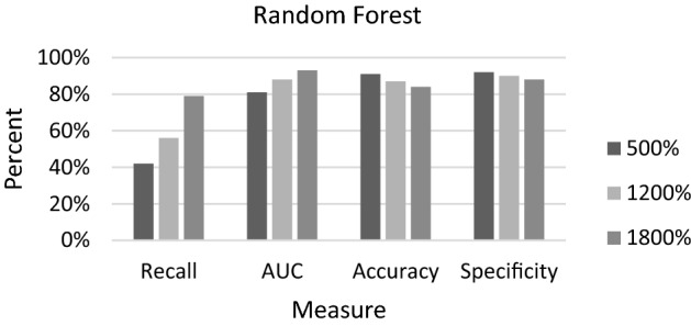
Recall, AUC, Accuracy and Specificity of Random Forest as oversampling percent is increased

In addition, for each measure we compared the classification performance of the three methods as the oversampling percentage was increased. As the oversampling percentage was increased, all classifiers showed an increase in recall with RF having the highest recall at 1800% SMOTE (79%), followed by C4.5 (78%) and ANN (76%) (Fig. 4). When the training set was not oversampled, all three classifiers had a 0% recall on the test set.

Fig. 4.

Recall of C4.5, Neural Network and Random Forest as oversampling percent is increased

For the AUC, at 1800% SMOTE, RF had the highest value (93%) followed by C4.5 (91%) and ANN (84%). When the training set was not oversampled, C4.5, Neural Network and Random Forest had AUC values of 52%, 69% and 74%, respectively (Fig. 5).

Fig. 5.

AUC of C4.5, Neural Network and Random Forest as oversampling percent is increased

Looking at the accuracy plot (Fig. 6), we can see that Random Forest had the highest value (84%) at 1800% SMOTE followed by C4.5 (82%) and Neural Network (77%). When the training set was not oversampled, the accuracy of C4.5, ANN and RF were 98%, 97% and 96%, respectively. This is due to the highly imbalanced nature of the original data which makes it much easier for the classifier to correctly identify the majority group.

Fig. 6.

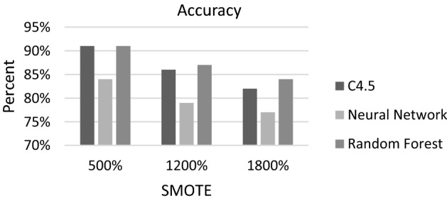
Accuracy of C4.5, Neural Network and Random Forest as oversampling percent is increased

Using specificity, we observed similar results to accuracy where the specificity of all three classifiers decreased as the oversampling percentage was increased (Fig. 7). Also, at 1800% SMOTE, Random Forest had the highest specificity (88%) followed by C4.5 (82%) and Neural Network (78%). When the minority group was not oversampled, each of the classifiers had a specificity of 99% or 100% due to the highly imbalanced nature of the data where 96.87% of instances are from the majority group.

Fig. 7.

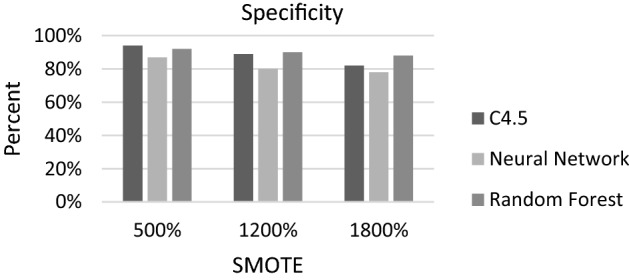
Specificity of C4.5, Neural Network and Random Forest as oversampling percent is increased

Figures 8, 9 and 10 show the ROC plot across the three classifiers for each oversampling percentage separately. Across all oversampling percentages, Random Forest has the highest AUC followed by C4.5 and Neural Network.

Fig. 8.

ROC of C4.5, Neural Network and Random Forest at 500% SMOTE

Fig. 9.

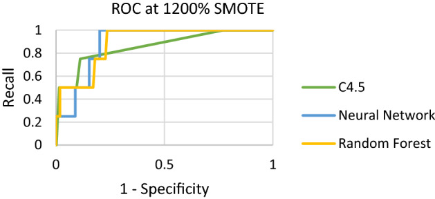
ROC of C4.5, Neural Network and Random Forest at 1200% SMOTE

Fig. 10.

ROC of C4.5, Neural Network and Random Forest at 500% SMOTE

Discussion

Overall, Random Forest was the best classifier as it had the highest recall, AUC, accuracy, and specificity at SMOTE of 1800%. While Neural Network is the most commonly used classifier in the sports analytics literature, our results show that it is not the best classifier. In fact, both C4.5 and Random Forest had a better performance than the Neural Network classifier across all measures. Given the simplicity and ease of interpretation of C4.5 and Random Forest, this increases the applicability of our findings. Our work also shows the importance of accounting for the data imbalance issue. After oversampling was applied, the classification performance of all classifiers significantly improved in identifying the minority group. Moreover, our work shows the ability to use publicly available data collected during the regular season to classify the winner of the Superbowl.

Our results can be used to develop a decision support tool to help team managers and coaches in developing strategies that can increase the team’s chances of winning by making data driven decisions regarding game plans, play selection and player recruitment. Furthermore, our approach, of accounting for the data imbalance issue using SMOTE before applying the classification algorithms, is generalizable so it can be used in other sports and non-sport fields.

Conclusions and future work

Although there is numerous research in the sports analytics field, they suffer from low accuracy. Moreover, although the NFL is the largest sports league in terms of revenue, it lags other professional sports in terms of analytics. According to the existing literature in sports analytics, more accurate models are needed and one of the recommendations for future research in the field is to utilize other data mining techniques. This works attempts to answers these calls and address some of the gaps in the existing literature by comparing the classification performance of C4.5, ANN and RF in classifying the winner of the Superbowl using data collected during the regular season. The data was split into a training set and a test set. SMOTE was used to oversample the minority group of the training set before C4.5, ANN and RF were applied. The classification performance of the three classifiers was compared on the test set using recall, AUC, accuracy and specificity. Overall, Random Forest had the best performance followed by C4.5 and Neural Network.

This study has several limitations. We only considered SMOTE for addressing the data imbalance issue so future studies should consider other approaches. We also compared only three classifiers, so we recommend future studies to consider more classifiers. We used data collected during the regular season to classify the winner of the Superbowl without considering playoffs games. A lot can happen between the end of the season and the final whistle of the Superbowl, such as injuries, so future research should try to consider these issues when attempting to predict the Superbowl winner. Our results are based on data from 18 seasons, so we recommend future studies to consider data from more seasons. We did not consider player level data which are important indicators and measures of team performances. Moreover, every season new players are drafted and players are traded so considering player level data would allow us to account for these season to season variations.

Nevertheless, our work has several significant implications. We highlight the imbalance issue of sports data consisting mainly of losing teams and we show the importance of considering methods for addressing this issue. Our results confirm results obtained by Bunker and Susjnak (2022) who showed that ANNs do not always perform the best even though they are the most popular technique. In our work, we show how C4.5 and Random Forest outperform ANNs which indicates the importance of using several classification techniques rather than relying on one popular technique.

Appendix

References

- Alamar B. Sports analytics. Columbia University Press; 2013. [Google Scholar]
- Baker RD, McHale IG. Forecasting exact scores in National Football League games. International Journal of Forecasting. 2013;29(1):122–130. doi: 10.1016/j.ijforecast.2012.07.002. [DOI] [Google Scholar]
- Baker RE, Kwartler T. Sport analytics: Using open source logistic regression software to classify upcoming play type in the NFL. Journal of Applied Sport Management. 2015;7(2):43–58. [Google Scholar]
- Biau G, Scornet E. A random forest guided tour. Test. 2016;25(2):197–227. doi: 10.1007/s11749-016-0481-7. [DOI] [Google Scholar]
- Bunker R, Susnjak T. The application of machine learning techniques for predicting match results in team sport: A review. Journal of Artificial Intelligence Research. 2022;73:1285–1322. doi: 10.1613/jair.1.13509. [DOI] [Google Scholar]
- Bunker RP, Thabtah F. A machine learning framework for sport result prediction. Applied Computing and Informatics. 2019;15(1):27–33. doi: 10.1016/j.aci.2017.09.005. [DOI] [Google Scholar]
- Burke, B. (2019). DeepQB: deep learning with player tracking to quantify quarterback decision- making & performance. In Proceedings of the 2019 MIT Sloan Sports Analytics Conference
- Cao, C. (2012). Sports data mining technology used in basketball outcome prediction. Masters Dissertation. Technological University Dublin.
- Carpita M, Ciavolino E, Pasca P. Exploring and modelling team performances of the Kaggle European Soccer database. Statistical Modelling. 2019;19(1):74–101. doi: 10.1177/1471082X18810971. [DOI] [Google Scholar]
- Chawla NV, Bowyer KW, Hall LO, Kegelmeyer WP. SMOTE: Synthetic minority over-sampling technique. Journal of Artificial Intelligence Research. 2002;16:321–357. doi: 10.1613/jair.953. [DOI] [Google Scholar]
- Delen D, Cogdell D, Kasap N. A comparative analysis of data mining methods in predicting NCAA bowl outcomes. International Journal of Forecasting. 2012;28(2):543–552. doi: 10.1016/j.ijforecast.2011.05.002. [DOI] [Google Scholar]
- Gepp A, Kumar K, Bhattacharya S. Business failure prediction using decision trees. Journal of Forecasting. 2010;29(6):536–555. doi: 10.1002/for.1153. [DOI] [Google Scholar]
- Haghighat M, Rastegari H, Nourafza N, Branch N, Esfahan I. A review of data mining techniques for result prediction in sports. Advances in Computer Science: An International Journal. 2013;2(5):7–12. [Google Scholar]
- He H, Garcia EA. Learning from imbalanced data. Knowledge and Data Engineering IEEE Transactions on. 2009;21(9):1263–1284. doi: 10.1109/TKDE.2008.239. [DOI] [Google Scholar]
- Howington EB, Moates KN. Is there a bye week advantage in college football? Electronic Journal of Applied Statistical Analysis. 2017;10(3):735–744. [Google Scholar]
- Joash Fernandes C, Yakubov R, Li Y, Prasad AK, Chan TC. Predicting plays in the National Football League. Journal of Sports Analytics. 2020;6(1):35–43. doi: 10.3233/JSA-190348. [DOI] [Google Scholar]
- Kahn J. Neural network prediction of NFL football games. World Wide Web electronic publication. 2003;9:15. [Google Scholar]
- Kantardzic M. Data mining: Concepts, models, methods, and algorithms. Wiley; 2011. [Google Scholar]
- Kuhn M. Building predictive models in R using the caret package. Journal of Statistical Software. 2008;28:1–26. doi: 10.18637/jss.v028.i05. [DOI] [Google Scholar]
- LeDell, E., & Poirier, S. (2020, July). H2o automl: Scalable automatic machine learning. In Proceedings of the AutoML Workshop at ICML (Vol. 2020).
- Lock D, Nettleton D. Using random forests to estimate win probability before each play of an NFL game. Journal of Quantitative Analysis in Sports. 2014;10(2):197–205. doi: 10.1515/jqas-2013-0100. [DOI] [Google Scholar]
- Mamode Khan N, Sunecher Y, Jowaheer V. Modelling football data using a GQL algorithm based on higher ordered covariances. Electronic Journal of Applied Statistical Analysis. 2017;10(3):654–665. [Google Scholar]
- Menardi G, Torelli N. Training and assessing classification rules with imbalanced data. Data Mining and Knowledge Discovery. 2014;28(1):92–122. doi: 10.1007/s10618-012-0295-5. [DOI] [Google Scholar]
- Nayak, R., Jain, L. C., & Ting, B. K. H. (2001). Artificial neural networks in biomedical engineering: A review. Computational Mechanics–New Frontiers for the New Millennium, 1, 887–892.
- Ötting, M. (2020). Predicting play calls in the National Football League using hidden Markov models. arXiv preprint arXiv:2003.10791.
- Pujol JCF, Pinto JMA. A neural network approach to fatigue life prediction. International Journal of Fatigue. 2011;33(3):313–322. doi: 10.1016/j.ijfatigue.2010.09.003. [DOI] [Google Scholar]
- Purucker MC. Neural network quarterbacking. Ieee Potentials. 1996;15(3):9–15. doi: 10.1109/45.535226. [DOI] [Google Scholar]
- Quenzel J, Shea P. Predicting the winner of tied national football league hames: Do the details matter? Journal of Sports Economics. 2016;17(7):661–671. doi: 10.1177/1527002514539688. [DOI] [Google Scholar]
- Ramchoun, H., Ghanou, Y., Ettaouil, M., & Janati Idrissi, M. A. (2016). Multilayer perceptron: Architecture optimization and training. International Journal of Interactive Multimedia and Artificial Intelligence, 4(1), 26–30
- Reyers, M., & Swartz, T. B. (2022). Quarterback evaluation in the national football league using tracking data. AStA Advances in Statistical Analysis, 106, 1–16.
- Roumani YF, Roumani Y, Nwankpa JK, Tanniru M. Classifying readmissions to a cardiac intensive care unit. Annals of Operations Research. 2018;263(1):429–451. doi: 10.1007/s10479-016-2350-x. [DOI] [Google Scholar]
- Rudrapal D, Boro S, Srivastava J, Singh S. Computational Intelligence in Data Mining. Singapore: Springer; 2020. A deep learning approach to predict football match result; pp. 93–99. [Google Scholar]
- Torgo L. Data Mining with R, learning with case studies. Chapman and Hall/CRC; 2010. [Google Scholar]
- Wang X, Zhou C, Xu X. Application of C4.5 decision tree for scholarship evaluations. Procedia Computer Science. 2019;151:179–184. doi: 10.1016/j.procs.2019.04.027. [DOI] [Google Scholar]
- Wu YC, Feng JW. Development and application of artificial neural network. Wireless Personal Communications. 2018;102(2):1645–1656. doi: 10.1007/s11277-017-5224-x. [DOI] [Google Scholar]
- Xia, V., Jain, K., Krishna, A., & Brinton, C. G. (2018). A network-driven methodology for sports ranking and prediction. In 2018 52nd Annual Conference on Information Sciences and Systems (CISS) (pp. 1–6). IEEE.
- Zhou L. Performance of corporate bankruptcy prediction models on imbalanced dataset: The effect of sampling methods. Knowledge-Based Systems. 2013;41:16–25. doi: 10.1016/j.knosys.2012.12.007. [DOI] [Google Scholar]