Estimating mixture effects and cumulative spatial risk over time simultaneously using a Bayesian index low‐rank kriging multiple membership model

Abstract

The exposome is an ideal in public health research that posits that individuals experience risk for adverse health outcomes from a wide variety of sources over their lifecourse. There have been increases in data collection in the various components of the exposome, but novel statistical methods are needed that capture multiple dimensions of risk at once. We introduce a Bayesian index low‐rank kriging (LRK) multiple membership model (MMM) to simultaneously estimate the health effects of one or more groups of exposures, the relative importance of exposure components, and cumulative spatial risk over time using residential histories. The model employs an MMM to consider all residential locations for subjects weighted by duration and LRK to increase computational efficiency. We demonstrate the performance of the Bayesian index LRK‐MMM through a simulation study, showing that the model accurately and consistently estimates the health effects of one or several group indices and has high power to identify a region of elevated spatial risk due to unmeasured environmental exposures. Finally, we apply our model to data from a multicenter case‐control study of non‐Hodgkin lymphoma (NHL), finding a significant positive association between one index of pesticides and risk for NHL in Iowa. Additionally, we find an area of significantly elevated spatial risk for NHL in Los Angeles. In conclusion, our Bayesian index LRK‐MMM represents a step forward toward bringing the ideals of the exposome into practice for environmental risk analyzes.

1. INTRODUCTION

An emerging perspective in public health research is that of the exposome, ¹ which is the idea that individuals are susceptible to risk for adverse health outcomes from a variety of sources over their lifecourse. Three broad domains of the exposome are internal factors, specific external factors, and general external factors. Internal factors operate uniquely on an individual. Specific external factors include occupational and environmental exposures and lifestyle choices. General external factors are the most socially constructed and include educational attainment and socio‐economic class. ² A more comprehensive assessment of exposures offers several advantages over single‐exposure analysis. For one, it estimates the effects of a broader set of exposures across domains and/or time, in contrast to estimating the effects of one exposure in isolation. This more accurately depicts the experience of individuals throughout their lifecourse. ³ Models of risk that are designed to address the exposome must handle multidimensional exposure data. Such multidimensional data have increased in availability, owing to factors such as the increased measurement of biomarkers ⁴ as well as chemical or socio‐demographic exposures. In turn, this has increased the need for the development of models that can more comprehensively assess risk.

Two general classes of modeling approaches that address separate components of risk are mixture analysis and spatial analysis. In mixture analysis, multidimensional exposures are measured and analyzed together. Generally, this approach defines and measures exposure to a mixture of variables of some type, evaluates the health effect of exposure to the mixture, and ideally identifies the most important variables among the mixture for association with the outcome. Such an approach is preferable to a single‐exposure analysis because it acknowledges that not one but many exposures act upon individuals concurrently and adjusts for this in the estimation of exposure effects. In mixture analysis, the mixture components are typically environmental chemicals, ⁵ , ⁶ , ⁷ , ⁸ , ⁹ owing to their ubiquity in consumer products ¹⁰ and presence as airborne pollutants or in agricultural pesticides, but they could also consist of socio‐demographic variables. ¹¹ , ¹² , ¹³ Owing to the similarities in structure of some chemicals, and the use of multiple chemicals in certain products, there may be high correlations between many chemicals in a mixture, and this lack of independence requires additional care in modeling. Several approaches have been developed to assess the effects of correlated exposures in a mixture analysis. Bayesian kernel machine regression models use a smooth kernel function for each exposure‐response relationship, and have been used, for example, to assess the effects of several prenatal metal concentrations on childhood cardio‐metabolic risk. ¹⁴ Additionally, quantile g‐computation utilizes theories from causal inference to provide estimates of exposure mixtures, by adopting standard assumptions of causal identification (including causal consistency, no interference, and absence of unmeasured confounding) in order to estimate effects that would be obtained in a hypothetical randomized trial in which the treatment consisted of modifying the quantiles of all exposures of interest. ¹⁵ However, the extent to which the assumptions of causal analysis are satisfied in observational studies is unclear. Finally, the Bayesian group index model estimates the health effects of multiple groups of exposures and the importance weights of each component of an index within a Bayesian modeling framework. ¹⁶ The model was developed to build upon weighted quantile sum (WQS) regression, which sought to identify “bad actor” chemicals among a mixture but was not designed to handle multiple groups of exposures with differing effects in magnitude and direction and had inherently lower power due to the data splitting required in the method's two‐step estimation. Notable advantages to this model include its ability to estimate the health effects for each exposure group, as well as the full posterior distributions of all quantities of interest via Bayesian inference.

Spatial risk analyzes acknowledge that all relevant exposures may not be explicitly measured, but risk may derive from unmeasured exposures associated with residing in an area. Spatial risk studies have attempted to reveal patterns associated with unmeasured exposures retroactively, using case‐control data to determine whether a region confers elevated risk of being a case upon study participants, after controlling for a set of participant covariates known or suspected to be associated with the outcome. ¹⁷ , ¹⁸ , ¹⁹ , ²⁰ , ²¹ One limitation of past spatial cluster studies is using only one residential location for subjects, typically at the time of diagnosis. Recent additions to the literature such as the convolution multiple membership model ²² and low‐rank kriging multiple membership model ²¹ have broadened the set of residential locations under study to include complete residential histories, allowing estimation of cumulative spatial risk over time. These models allow all of a subject's residences, aggregated to larger administrative units or using point locations, respectively, to factor in to the subject's spatial random effect term in the model, weighted by the proportion of time they lived at each residence. The latter model uses low‐rank kriging to decrease the computational burden of using many point locations by simplifying the representation of the spatial process into a lower dimension. ²³ , ²⁴ A cluster of persisting elevated spatial risk in some area detected by models that utilize residential histories could spur epidemiologic investigation into potential causes of the elevated risk and potentially drive subsequent remediation efforts to address it. Consideration of spatial risk that is cumulative provides a more accurate estimate of environmental risk accumulated over the life course. ²¹ , ²² Though collecting and utilizing complete residential histories requires more effort, the feasibility of doing so retroactively has increased as LexisNexis and other public record databases have reasonable accuracy in replicating residential histories collected during a study of a geographically diverse set of individuals in the United States. ²⁵ , ²⁶

While mixture analysis and spatial risk analysis each address an important component of the exposome, they have not yet been considered together in an integrated modeling approach. In this article, we propose integrating these classes of environmental risk assessment into a Bayesian index low‐rank kriging multiple membership model (Bayesian index LRK‐MMM) that allows for their simultaneous estimation in a case‐control study where multiple measured environmental exposures and residential histories are present. As the name suggests, the model combines a Bayesian index model for mixture analysis with an LRK‐MMM that estimates cumulative and inherently latent spatial risk using residential histories. This Bayesian model provides a computationally efficient approach to estimating the effects of one or more groups of measured exposures while estimating cumulative spatial risk over time in a study area and adjusting for potential confounding variables. To evaluate the proposed model, we perform an extensive simulation study to assess its ability to simultaneously estimate group index health effects and cumulative spatial risk effects accurately. We then apply the Bayesian index LRK‐MMM to the National Cancer Institute's Surveillance, epidemiology, and end results non‐Hodgkin lymphoma (NCI‐SEER NHL) case‐control study to assess the effects of several groups of chemical exposures and residential histories within four geographically‐diverse study centers in the United States.

2. METHODS

2.1. Model specification

Acknowledging that individuals are exposed to both measured and unmeasured environmental risks for disease over time, we sought to combine both components in a single low‐rank kriging multiple membership model (Bayesian index LRK‐MMM). In a case‐control setting, we model the probability of being a case using a Bernoulli distribution for any subject. Specifically, for the ith subject, their case membership is an unchanging binary variable that has the distribution $Y_i\sim \mathit{\text{Bernoulli}}\left(p_i\right)$, where the logit of the probability is given by

$$\mathit{log}\left(\frac{p_i}{1-p_i}\right)={\mathrm{\beta }}_0+{\sum }_{j=1}^C{\mathrm{\beta }}_j{\sum }_{k=1}^{C_j}{\mathrm{\omega }}_{\mathit{jk}}{q}_{\mathit{ijk}}+{\sum }_{b=1}^B{\mathrm{\theta }}_b{x}_{\mathit{ib}}+{\sum }_{j\in A_{(i)}}{w}_{\mathit{ij}}{\sum }_{m=1}^{n_K}{\mathrm{\psi }}_{m}C\left[\left|s_{\mathit{ij}}-k_m\right|/\mathrm{\rho }\right].$$

We begin by describing the chemical exposure and covariate components of the model. Here, ${\mathrm{\beta }}_0$ is an intercept term, and $\left[{\mathrm{\beta }}_1,\dots ,{\mathrm{\beta }}_C\right]$ are the set of regression coefficients (exposure‐related health effects) for the $C$ chemical indices in the model. For the jth chemical index, the importance weights are $\left[{\mathrm{\omega }}_{j1},\dots ,{\mathrm{\omega }}_{j{C}_j}\right]$, which are subject to the constraint ${\sum }_{k=1}^{C_j}{\mathrm{\omega }}_{\mathit{jk}}=1$, and the chemicals in the index are scored into quantiles (eg, quartiles 0, 1, 2, 3) in order to reduce collinearity between chemicals in the index and accommodate different scales for the chemicals. ²⁷ , ²⁸ Therefore, the quantity $q_{\mathit{ijk}}$ denotes the kth chemical in the jth chemical index for the ith subject. The term ${\sum }_{b=1}^B{\mathrm{\theta }}_B{x}_{\mathit{ib}}$ incorporates a set of covariates or control variables $\left[x_{i1},\dots ,x_{\mathit{iB}}\right]$ and their associated coefficients $\left[{\mathrm{\theta }}_1,\dots ,{\mathrm{\theta }}_B\right]$. For simplicity, we do not include covariates in the design of the simulation study, but they are included in the data application.

The spatial risk component of the model is designed to estimate the cumulative spatial risk incurred by participants with respect to risk of case membership over their residential histories. The set $\left\{{\mathrm{\kappa }}_1,\dots ,{\mathrm{\kappa }}_{n_K}\right\}$ gives the $n_K$ knot locations that represent the geographic distribution of case and control locations. The knot locations are chosen by some knot selection algorithm, which we discuss in detail below. The ith subject's set of residential histories is denoted by $A_{(i)}=\left[s_{i1},\dots ,s_{\mathit{iJ}}\right]$, and the proportion of time that this subject lived in those locations is $\left[w_{i1},\dots ,w_{\mathit{iJ}}\right],$ where ${\sum }_{j=1}^J{w}_{\mathit{ij}}=1$. Thus, the weight $w_{\mathit{ij}}$ represents the proportion of time that the ith individual lived in the jth residential location and indicates the proportion of the time of cumulative spatial risk this individual derived from this location. The set of spatially‐structured random effects is $\left[{\mathrm{\psi }}_1,\dots ,{\mathrm{\psi }}_{n_K}\right],$ where each element of $\mathrm{\psi }$ is evaluated at one of the knot locations chosen by the knot selection algorithm. The function $C[·]$ is a Matern covariance function that simplifies to $C[t]=(1+\left|t\right|)e^{-\left|t\right|}$ when fixing parameters of the Matern family of $m$ and $\mathrm{\nu }$ to $1$ and $\frac{3}{2}$, respectively. We choose to use the Matern family of covariance functions here due to its popularity in geostatistical models in the literature, ²⁹ , ³⁰ as well as its smoothness and flexibility.

2.2. Knot selection

Reducing the dimensionality of the spatial risk component of the Bayesian index LRK‐MMM requires the evaluation of spatial random effects at the knot locations, which are chosen by some knot selection algorithm. One method to simplify a spatial process through using knots is known as low‐rank kriging (LRK). Previously, LRK models have commonly used the space‐filling algorithm to choose knot locations. This algorithm seeks to minimize a geometric space‐filling function of distances between points taken over the area of interest. ³¹ , ³² , ³³ , ³⁴ , ³⁵ However, when analyzing data from a case‐control setting, more recent research has demonstrated that other knot selection algorithms allow models a greater spatial sensitivity and power to identify regions of elevated spatial risk for disease. ³⁶ One such algorithm is the heuristic of Teitz and Bart, ³⁷ which addresses the location‐allocation problem in operations research, where the objective function to be minimized is the total distance between a set of clients and the facility locations that serve them. This algorithm has been described previously ²¹ and has demonstrated improvements in spatial power and sensitivity to identify regions of elevated risk for disease for case‐control studies. ²¹ , ³⁸ In all models fit for this article, we chose knot locations using the Teitz and Bart heuristic, considering the case residential locations to constitute the set of clients and knot locations to constitute the facilities.

2.3. Simulation study design

2.3.1. Data‐generating process

We designed a simulation study to cover a variety of plausible scenarios where risk derives from both exposure to a mixture of chemicals at one time (eg, measured inside the home after study enrollment) and a spatial process that represents unmeasured exposures over a long duration of time. We simulated 20‐year residential histories over a study region, and activated a circular zone of elevated spatial risk for disease of radius 50 km in the study region for the first 5 years of the study period, that is, ending 15 years before study enrollment. Simulated participants living in the zone of elevated risk when it was active experienced a one‐time increase of 1.5 on the log‐odds scale in risk for disease relative to those who did not live in the zone when it was active.

In separate classes of simulation scenarios, we added a measurable chemical risk consisting of one or three groups of chemicals. In a given class, we simulated concentrations for 27 chemicals in an index from two different correlation structures: a first‐order autoregressive correlation matrix, and the correlation matrix between chemicals measured in the NCI‐SEER NHL study (described in further detail below). The number of chemicals for which we simulated concentrations is based on the number of chemicals measured in the NCI‐SEER NHL study, which were measured at one time inside the homes of study participants. Numbering the chemicals from $1$ to $27$, then, the correlation between the ith and jth chemicals in the autoregressive structure was $r^{\left|i-j\right|}$. In separate scenarios, we used values of $0.75$ and $0.50$ for $r$ to explore the effect of differing levels of autoregressive correlation between chemicals on model performance. The empirical correlation matrix, derived from the chemicals measured in the NCI‐SEER study, contained some missing data, which generally occurred when the concentration of a chemical fell below the detection limit of the instrument used to measure it. Assuming the chemical concentrations followed log‐normal distributions, missing values were imputed 10 times with a “fill‐in” approach to create a complete dataset, and we drew one of the imputed datasets at random. Details on the imputation of these chemicals can be found elsewhere. ³⁹ , ⁴⁰ , ⁴¹ Owing to some large correlations between pairs of these chemicals that could impact model stability, we also simulated chemical concentrations from a dampened correlation matrix defined as $C_1=0.65*\left(C_0-I\right)+I$, where $C_0$ is the observed original correlation matrix and $I$ is the identity matrix. We chose the dampening constant 0.65 to retain moderate correlation from the empirical matrix.

We then set the importance weights for chemicals in the indices. For the one‐index model, when the autoregressive correlation structure was used, the importance weights were $[\mathrm{0.40,0.25,0.15,0.10,0.10}]$ for the first five chemicals, and zero for the remaining 22 chemicals, and when the empirical correlation structure was used, the importance weights were $\pi =\left[\begin{array}{c}\mathrm{0.02,\; 0.003,\; 0.02,\; 0.03,\; 0.32,\; 0.002,\; 0.06,\; 0.004,\; 0.07,\; 0.003,\; 0.01,\; 0.002,\; 0.035,\; 0.07},\\ \mathrm{0.01,\; 0.003,\; 0.001,\; 0.03,\; 0.001,\; 0.08,\; 0.001,\; 0.003,\; 0.002,\; 0.005,\; 0.035,\; 0.01,\; 0.17}\end{array}\right]$, based on the estimated importance weights for the one‐chemical index in a previous analysis of chemical mixtures on NHL risk. ³⁹ For the three‐index model, the three indices had sizes $C_1=5,C_2=7,C_3=15$. When the autoregressive correlation structure was used, the importance weights were $w_1=[\mathrm{0.40,0.10,0.10,0.20,0.20}],w_2=[\mathrm{0.05,\; 0.10,\; 0.15,\; 0.40,\; 0.15,\; 0.10,\; 0.05}],w_3=[\mathrm{0.01,\; 0.02,\; 0.03,\; 0.04,\; 0.04,\; 0.04,\; 0.05,\; 0.05,\; 0.06,\; 0.07,\; 0.08,\; 0.09,\; 0.10,\; 0.14,\; 0.18}]$.

When the empirical correlation structure was used, the importance weights in the first index were ${\mathrm{\pi }}_{1k}={\mathrm{\pi }}_k/{\sum }_{k=1}^5{\mathrm{\pi }}_k$, the importance weights in the second index were ${\mathrm{\pi }}_{2k}={\mathrm{\pi }}_k/{\sum }_{k=6}^{12}{\mathrm{\pi }}_k$, and the importance weights in the third index were ${\mathrm{\pi }}_{3k}={\mathrm{\pi }}_k/{\sum }_{k=13}^{27}{\mathrm{\pi }}_k$.

Finally, we varied the health effects (regression coefficients) of the chemical indices in the following manner. For the one‐index model, we defined ${\mathrm{\beta }}_1=[\mathrm{2,1.25,0.5}]$ in separate scenarios. For the three‐index model, we used three sets of regression coefficients: $\mathrm{\beta }=[(1,-\mathrm{1.5,0}),(1,1,0),(\mathrm{2,0.5,0})]$ to explore the effects of varying magnitudes and directions of health effects on the model's performance.

2.3.2. Model fitting

We fitted a Bayesian index LRK‐MMM to every simulated dataset, using $n_K=60$ knots in all scenarios, which was adequate to cover the study region and minimize distance from cases to knot locations to a reasonable extent while considering computational costs. We fitted models in the Bayesian paradigm using Markov chain Monte Carlo (MCMC) methods. We complete the specification of the Bayesian index LRK‐MMM by specifying the prior distributions of parameters in the model. All regression parameters ${\mathrm{\beta }}_i$ received a vague Normal prior ${\mathrm{\beta }}_i\sim N\left(0,\mathrm{\tau }={10}^{-3}\right)$, where $\mathrm{\tau }$ denotes the precision, which is the reciprocal of the variance. The random effects $\mathrm{\psi }$ received a multivariate normal prior $\mathit{MVN}\left(0,{\mathrm{\tau }}_S{\mathrm{\Omega }}^{-1}\right)$, using precision matrix $\mathrm{\Omega }=\left[C\left[\left|k_a-k_b\right|/\mathrm{\rho }\right]\right],1\le a,b\le n_K$, with the same Matern covariance function $C[·]$ as above, and ${\mathrm{\tau }}_s=\frac{1}{{\mathrm{\sigma }}_S^2}$ where ${\mathrm{\sigma }}_s\sim \mathit{\text{Unif}}(0,10)$. The spatial correlation parameter $\mathrm{\rho }$ was assigned a vague $\mathit{\text{Uniform}}(0,30)$ prior. The chemical importance weights had a Dirichlet prior with parameters $\mathrm{\alpha }=\left[{\mathrm{\alpha }}_1,\dots ,{\mathrm{\alpha }}_{C_j}\right]$ in order that the chemical weights in a given chemical index were between $0$ and $1$ and ${\sum }_{j=1}^{C_j}{\mathrm{\omega }}_{\mathit{ij}}=1$. We did not consider adjustment covariates in the simulation study. We estimated models using just another Gibbs sampler (JAGS) ⁴² in the software R, version 3.6.1. ⁴³ In the MCMC simulations, each model used two chains that each burned in 50 000 iterations and sampled 30 000 additional observations from the posterior distribution. We checked for convergence of parameters in the model by the Gelman‐Rubin statistic, considering a parameter to have converged if its Gelman‐Rubin statistic was less than 1.1, ⁴⁴ using the coda R package. ⁴⁵ We used the posterior samples of $\mathrm{\psi }$ and the covariance function to predict the spatial odds ratio for disease on a fine grid covering the study region. In doing so, we generated a posterior distribution of spatial odds at each grid cell. Each grid cell approximately represented a 6 km² area in the study region. We concluded that a grid cell had significantly elevated or lowered spatial risk for disease using exceedance probabilities, ⁴⁶ which use the posterior distribution to estimate the frequency at which spatial odds at a grid cell depart from the null value of 1. Grid cells having exceedance probability greater than or equal to $0.95$ of being greater or lesser than 1 were considered to be of significantly elevated or lowered risk, respectively.

2.3.3. Model evaluation

We evaluated model performance with respect to both the chemical and spatial components. For the spatial risk component, we used the posterior distribution of spatial odds ratios at grid cells covering the study region. Defining the grid cells inside of the zone of elevated risk to constitute the set $S$, we defined the spatial sensitivity of the model for the dth dataset as $\mathit{se}{n}_d=\frac{1}{\left|S\right|}{\sum }_{s_i\in S}I\left(\widehat{q_{s_i}}>0.95\right)$, where $\widehat{q_{s_i}}$ is the estimate of the exceedance probability at grid cell $s_i$, and $I(·)$ represents an indicator function. We also calculated spatial specificity. Defining the grid cells outside the zone of elevated risk to constitute the set $\mathit{NS}$, we defined the spatial specificity of the model for the dth dataset as $\mathit{spe}{c}_d=\frac{1}{\left|\mathit{NS}\right|}{\sum }_{n{s}_i\in \mathit{NS}}\left(1-I\left(\widehat{q_{n{s}_i}}>0.95\right)\right)$. We averaged the spatial sensitivity and specificity over $D=50$ datasets. Finally, we calculated spatial power according to a sensitivity threshold of zero, considering the model to have identified the zone of elevated risk if it identified any grid cells in the zone as having elevated risk, and calculating the spatial power as $P=\frac{1}{D}{\sum }_{d=1}^{D}I\left(\mathit{se}{n}_d>0\right)$.

For the chemical risk component, we considered the model's accuracy in both estimating the health effects and identifying the important chemicals in the index. In a given simulation scenario, we calculated the mean estimated health effect as $\widehat{\mathrm{\beta }}=\frac{1}{D}{\sum }_{d=1}^D\widehat{{\mathrm{\beta }}_d}$ in order to compare to the true health effect $\mathrm{\beta }$, and we also calculated the coverage probability of the health effect as $\frac{1}{D}{\sum }_{d=1}^{D}I\left(\mathrm{\beta }\in \left(\widehat{{\mathrm{\beta }}_{d,0.025}},\widehat{{\mathrm{\beta }}_{d,0.975}}\right)\right)$, where $\widehat{{\mathrm{\beta }}_{d,q}}$ denotes the qth quantile of the posterior distribution for health effect $\mathrm{\beta }$ and dataset $d$. Finally, for the chemical importance weights, we defined importance as having a weight greater than the reciprocal of the number of chemicals in the index. We considered the model to have identified the kth chemical in the jth index as important if $\widehat{{\mathrm{\omega }}_{\mathit{jk}}}>\frac{1}{C_j}$, and as unimportant otherwise. For a given dataset, we calculated the chemical sensitivity as the proportion of truly important chemicals in an index that were identified as such, and the chemical specificity as the proportion of truly unimportant chemicals in the index that were identified as such. We also calculated mean square error (MSE) for chemicals in the jth group of the three‐group model as $\mathit{MS}{E}_j=\frac{1}{D}{\sum }_{d=1}^D\frac{1}{C_j}{\sum }_{j=1}^{C_j}{\left(\widehat{{\mathrm{\omega }}_{\mathit{jd}}}-{\mathrm{\omega }}_{\mathit{jd}}\right)}^2$.

2.4. Application to NCI‐SEER NHL study

We applied the Bayesian index‐LRK‐MMM to data from the National Cancer Institute (NCI) surveillance, epidemiology, and end results (SEER) NHL case‐control study to determine whether there existed significant associations between multiple chemical exposure indices and NHL, and if there existed significantly elevated regions of cumulative spatial risk for NHL. The NCI‐SEER NHL study is a multicenter and population‐based case control study of NHL in four varied areas of the United States (Wayne, Oakland, and Macomb Counties, comprising the Detroit metropolitan region; Los Angeles County; King and Snohomish Counties, comprising the Seattle metropolitan region; and the state of Iowa). The study population, which has been described in detail previously, ⁴⁷ , ⁴⁸ included 1321 cases of NHL that were diagnosed between July 1, 1998 and June 30, 2000, aged 20 to 74 years, and diagnosed at one of the above four SEER registries. Population‐based controls (1057) were selected among the residents of each SEER registry using random‐digit dialing for controls less than 65 years old and Medicare eligibility files for controls greater than or equal to 65 years. The controls were matched on frequency to the cases by age (within 5‐year groups), sex, race, and SEER registry. Controls reporting a history of either NHL or HIV were excluded from the study.

Study participants completed a lifetime residential history calendar, which asked participants to state the complete address of any home they lived in, beginning from birth and including temporary or vacation homes where they lived for a total of at least 2 years. Interviewers completed in‐person interviews with participants in which they reviewed the calendar with participants and attempted to resolve any discrepancies or missing data in the calendar. Residential addresses in the calendar were matched to databases of geographic addresses to obtain geographic coordinates. ⁴⁹ Interviewers took global positioning system (GPS) readings outside the home to obtain the coordinates for the current home.

We applied the Bayesian index LRK‐MMM to spatially model the probability that a study participant had NHL within each SEER study center area, treating NHL status as a binary response variable $Y$ taking values of $1$ and $0$ for cases and controls, respectively. We fitted models at each study center to allow for differences in chemical exposure profiles and strengths of association with NHL status in different regions of the country. We adjusted for age, gender (male vs. reference female), race (black or other vs. reference white), and level of education (college degree or high school degree vs. reference less than high school degree) in all models, as done in previous analyzes of the NCI‐SEER NHL study. ⁵ , ²⁰ , ⁴⁸

The NCI‐SEER Study measured chemical concentrations from samples of dust taken from vacuum cleaners of consenting participants. The details of this process have been described previously. ⁵ , ⁴⁰ We included four chemical indices in the Bayesian index LRK‐MMM: polychlorinated biphenyls (PCBs) (congeners 105, 138, 153, 170, 180); polycyclic aromatic hydrocarbons (PAHs) (Benz(a)anthracene, Benzo(a)pyrene, Benzo(b)fluoranthene, Benzo(k)fluoranthene, Chrysene, Dibenz(ah)anthracene, Indeno(1,2,3‐cd)pyrene); pesticides index I ($\mathrm{\alpha }$‐Chlordane, $\mathrm{\gamma }$‐Chlordane, Carbaryl, Dichlorodiphenyldichloroethylene (DDE), Dichlorodiphenyltrichloroethane (DDT), o‐phenylphenol, Pentachlorophenol, Propoxur); and pesticides index II (Chlorpyrifos, cis‐permethrin, trans‐permethrin, 2,4‐D, Diazinon, Dicamba, Methoxychlor). We chose this grouping of chemicals owing to its use in a previous chemical analysis of NHL risk based on univariate associations ⁵⁰ , ⁵¹ and scored chemical concentrations into quantiles ($q=0,1,2,3$) for each variable. To further assess the health effects of these chemical groups for NHL, we combined data from the four study centers into one model and omitted the spatial risk component for strictly a mixture analysis.

To address the spatial risk component of the model, we placed $n_k=60$ knots over the study region, choosing knot locations with the Teitz and Bart heuristic to minimize the objective function of total distance between case locations and the knots. This number of knots was sufficient to capture most of the population clustering across each study center, meaning that at least one knot was placed in any notably‐sized clustering of participants. Additionally, we conducted a sensitivity analysis by fitting models with an increasing series of knots (80, 100, and 130) to evaluate the effect of this choice on model performance in terms of deviance information criterion (DIC). ⁵² The results of this analysis, which we provide in the Appendix S1, indicate that 60 knots is a good choice when compared with the other numbers of knots because no other knot number leads to a better fitting model in all four study centers. We began with a random configuration of knot locations and iteratively changed the knot location set to other points on a fine grid covering the study region if doing so decreased the objective function. We stopped the algorithm when any possible improvement to the objective function was of less than three kilometers.

We specified the priors as in the simulation study, with two differences. First, we adjusted for several individual‐level covariates, assigning each a normal prior ${\mathrm{\theta }}_i\sim N\left(0,{\mathrm{\tau }}_i\right)$, where ${\mathrm{\tau }}_i=\frac{1}{{\mathrm{\sigma }}_i^2}$ and ${\mathrm{\sigma }}_i\sim \mathit{\text{Unif}}(0,10)$. Additionally, we allowed the precisions of each chemical group index to vary. Specifically, we assigned $B_i\sim \mathit{\text{Normal}}\left(0,{\mathrm{\tau }}_C\right)$ where ${\mathrm{\tau }}_c=\frac{1}{{\mathrm{\sigma }}_c^2}$ and ${\mathrm{\sigma }}_c\sim \mathit{\text{Unif}}(0,10)$. We fitted models in JAGS, using a burn‐in period of 80 000 iterations and retaining 50 000 for sampling from the joint posterior distribution. We performed inference on the chemical groups using their credible intervals, considering an association between chemical group and risk for NHL to be significantly positive (negative) if the 95% credible interval for the chemical index health effect fell above (below) zero. We assessed spatial risk over a 3 km‐by‐3 km grid over each study center, predicting the spatial risk at each grid cell using the posterior distribution of the spatial random effects evaluated at knot locations and the covariance function. We identified areas as being significantly elevated or lowered in risk as above, using a 90% exceedance probability threshold, which is a common threshold for these quantities in spatial epidemiology. ⁵³ In addition, we mapped the significance and spatial odds ratios for each grid cell for each study center in order to visually assess trends in spatial risk.

3. RESULTS

3.1. Simulation study

According to the coverage probabilities, the health effect $\mathrm{\beta }$ was captured in at least 90% of the simulated datasets for 10 of the 12 sub‐scenarios (Table 1). In the two sub‐scenarios having lower coverage probabilities, the magnitude of the health effect was large ($\mathrm{\beta }=2$), and the credible interval for the estimated coefficient fell above the true value. The health effect was estimated most accurately at the smallest magnitude of 0.5, with average estimated effects close to the true one, and larger effects were slightly over‐estimated with greater over‐estimation for larger magnitudes of the effects. For the autoregressive correlation structure, the health effects were estimated more accurately for the strong correlation set of scenarios ($\mathrm{r}=0.75$) than for the moderate correlation set of scenarios ($\mathrm{r}=0.50$), likely due to the fact that all of the important chemicals in the index were “proximate” and thus more likely to move strongly in one direction and provide a stronger signal. For the empirical correlation matrix, the health effect was estimated more accurately at high magnitudes for the un‐dampened matrix, and estimated more accurately at the lowest magnitude for the dampened correlation matrix, providing evidence that in the presence of smaller effect sizes, lower correlation between chemicals in the index allowed more precise estimation. At greater magnitudes, such de‐correlation was not as necessary for precise estimation. Figure 1 illustrates the true and estimated health effects across scenarios. The sensitivity and specificity of detecting the important chemicals in the index varied with respect to both the correlation structure and the magnitude of the health effect. For the autoregressive structure, the strongest correlations led to the greatest sensitivity and specificity, as high correlations between all important and proximate chemicals allowed them to move more in unison and be detected or not detected together. For the less structured empirical correlation matrix, dampening the magnitude of the correlation matrix led to improved sensitivity and specificity by separating the chemical signal from noise and allowing the detection of the important chemicals which often had low‐to‐moderate pairwise correlations. Table 2 displays the performance of the spatial risk component of the model. The mean spatial sensitivity ranged from 0.820 to 0.899 across all sub‐scenarios, indicating that the model often correctly identified a large proportion of the elevated risk area. The mean spatial specificity ranged from 0.809 to 0.951, indicating that the much of the study region that was not truly elevated in risk was correctly identified as having null spatial risk. The spatial power values of 1 in every sub‐scenario indicate that, in any simulated dataset for every sub‐scenario, the model correctly identified at least part of the zone of elevated risk.

TABLE 1.

Summary of chemical index estimates for model with one chemical group

			Chemicals in index		Overall mixture component
Correlation structure	Correlation strength	Beta for chemicals	Sensitivity	Specificity	Mean $\mathrm{\beta }$	Coverage
AR (1)	Strong	2	0.936	0.902	2.457	0.780
		1.25	0.904	0.756	1.346	0.920
		0.5	0.644	0.585	0.529	0.900
	Moderate	2	0.860	0.839	2.728	0.860
		1.25	0.716	0.720	1.375	0.960
		0.5	0.536	0.599	0.571	0.960
Like NHL data	Empirical	2	0.517	0.602	2.252	0.940
		1.25	0.473	0.568	1.415	0.960
		0.5	0.403	0.552	0.601	0.980
	0.65* Empirical	2	0.567	0.641	2.425	0.940
		1.25	0.520	0.593	1.499	0.940
		0.5	0.423	0.551	0.553	0.920

Note: 0.65* Empirical indicates the dampened correlation matrix.

FIGURE 1.

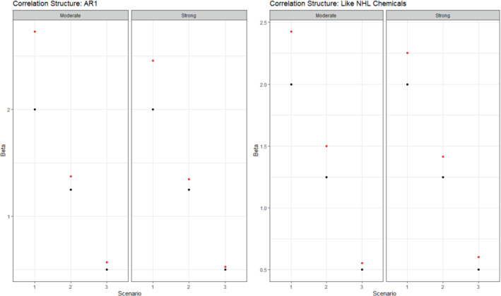
Summary of true (black) and estimated (red) betas for the one‐group model in the simulation study. Columns indicate different scenarios and exposure correlation strengths

TABLE 2.

Summary of spatial risk estimates for model with one chemical group

Correlation structure	Correlation strength	Beta for chemicals	Sensitivity	Specificity	Power
AR (1)	Strong	2	0.833	0.943	1.000
		1.25	0.830	0.916	1.000
		0.5	0.820	0.813	1.000
	Moderate	2	0.836	0.945	1.000
		1.25	0.860	0.913	1.000
		0.5	0.836	0.850	1.000
Like NHL data	Empirical	2	0.878	0.941	1.000
		1.25	0.899	0.889	1.000
		0.5	0.870	0.809	1.000
	0.65* Empirical	2	0.841	0.951	1.000
		1.25	0.869	0.925	1.000
		0.5	0.842	0.854	1.000

Note: Sensitivity and specificity for chemicals in one‐group index model. Threshold of importance is determined as $\frac{1}{J}$, where $J$ is the number of chemicals in the index.

Empirical indicates the dampened correlation matrix.

Extending the chemical risk component to comprise three indices, the model demonstrated an ability to estimate the effects of several mixtures that have true effects varying in magnitude and direction (Table 3). The estimated health effects are very close to the true ones for at least two of the three indices in all scenarios. Further, in contrast to Figure 1, which shows slight but frequent over‐estimation of the health effect in the one‐index model, Figure 2 illustrates no systematic bias of over‐ or under‐estimation of the health effects across scenarios. The coverage probabilities remain satisfactorily high, with 33 of 36 estimated coverage probabilities across health effects and scenarios equal to 0.92 or greater. Notably, the three‐index model remained able to accurately estimate health effects even in the presence of strong collinearity between chemicals in an index for the autoregressive $(\mathrm{r}=0.75)$ and empirical (undampened) correlation matrices. There is a slight increase in the MSEs of the estimated chemical weights for the autoregressive structure when decreasing the correlation between chemicals, which can be explained by a corresponding reduction in the chemical signal of proximate important chemicals in separate groups (Table 3). Using the empirical correlation matrix, dampening the correlation matrix is associated with a decrease in the MSEs of the estimated chemical weights. In general, the third health effect (having coefficient ${\mathrm{\beta }}_3=0$) had the smallest MSE for chemical weights, which is largely explained by many of the chemicals in this index having true importance weights that were small and similar to each other.

TABLE 3.

Summary of chemical index estimates for model with three chemical groups

			MSE for Chemical weights			Overall mixture component
Correlation structure	Correlation strength	${\mathrm{\beta }}_1,{\mathrm{\beta }}_2,{\mathrm{\beta }}_3$	Group 1	Group 2	Group 3	Mean ${\mathrm{\beta }}_1$	Cov.	Mean ${\mathrm{\beta }}_2$	Cov.	Mean ${\mathrm{\beta }}_3$	Cov.
AR (1)	Strong	1, −1.5, 0	0.0137	0.0099	0.0020	1.018	0.960	−1.680	0.980	−0.073	0.980
		1, 1, 0	0.0130	0.0117	0.0021	1.056	1.000	0.984	0.960	0.061	0.960
		2, 0.5, 0	0.0134	0.0128	0.0021	2.095	0.960	0.501	0.960	0.115	0.940
	Moderate	1, −1.5, 0	0.0134	0.0105	0.0025	1.059	0.960	−1.622	0.980	−0.081	0.960
		1, 1, 0	0.0150	0.0117	0.0023	0.891	0.940	1.050	0.960	−0.116	0.960
		2, 0.5, 0	0.0130	0.0134	0.0024	1.896	0.960	0.506	1.000	−0.142	0.960
Like NHL data	Empirical	1, −1.5, 0	0.0775	0.0331	0.0101	1.047	0.940	−1.664	0.900	0.090	0.980
		1, 1, 0	0.0755	0.0326	0.0099	1.032	0.960	0.999	0.840	0.026	0.980
		2, 0.5, 0	0.0312	0.0334	0.0103	2.166	0.920	0.453	0.920	−0.014	1.000
	0.65* Empirical	1, −1.5, 0	0.0596	0.0263	0.0102	1.081	0.960	−1.620	0.920	0.195	0.980
		1, 1, 0	0.0580	0.0288	0.0105	1.182	0.940	1.031	0.920	0.034	0.900
		2, 0.5, 0	0.0153	0.0331	0.0103	2.310	0.920	0.498	0.920	0.071	0.920

Note: Cov., coverage, the proportion of datasets with credible intervals containing true value of ${\mathrm{\beta }}_i,i=1,2,3;$ MSE, mean square error.

Empirical indicates the dampened correlation matrix.

FIGURE 2.

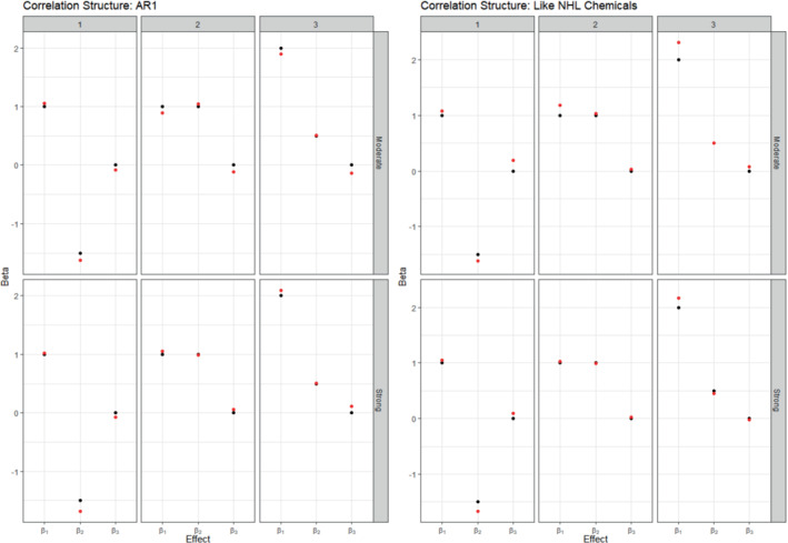
Summary of true (black) and average estimated (red) betas for the three‐group model in the simulation study. Columns indicate different scenarios and rows indicate different exposure correlation strengths

For the spatial risk component of the model, the mean spatial sensitivity ranged from 0.720 to 0.853 across scenarios, indicating that the model often correctly identified most of the zone of elevated risk (Table 4). The mean spatial specificity ranged from 0.871 to 0.978, meaning that the vast majority of the study region that was not truly elevated in risk was correctly categorized as having null risk. The spatial power values of at least 0.98 in every sub‐scenario indicate that, for all scenarios, the model only failed to detect the zone of elevated risk for at most one simulated dataset. In general, the spatial sensitivity values were slightly lower, and the spatial specificity values slightly higher, than their corresponding values in the one‐index model. This suggests that the three‐index model found fewer areas to have non‐null spatial risk, with more of the excess spatial variation in risk of being a case being attributed to the multiple chemical indices. The maintenance of near complete spatial power in this class of scenarios, however, demonstrates the Bayesian index LRK‐MMM's ability to consistently detect elevated spatial risk even in the presence of several other components in the model.

TABLE 4.

Summary of spatial risk estimates for model with three chemical groups

Correlation structure	Correlation strength	${\mathrm{\beta }}_1,{\mathrm{\beta }}_2,{\mathrm{\beta }}_3$	Sensitivity	Specificity	Power
AR (1)	Strong	1, −1.5, 0	0.843	0.871	1.000
		1, 1, 0	0.853	0.959	1.000
		2, 0.5, 0	0.813	0.972	1.000
	Moderate	1, −1.5, 0	0.809	0.877	1.000
		1, 1, 0	0.767	0.965	0.980
		2, 0.5, 0	0.720	0.978	0.980
Like NHL data	Empirical	1, −1.5, 0	0.798	0.962	0.980
		1, 1, 0	0.800	0.957	0.980
		2, 0.5, 0	0.737	0.963	0.980
	0.65* Empirical	1, −1.5, 0	0.815	0.948	1.000
		1, 1, 0	0.828	0.960	1.000
		2, 0.5, 0	0.776	0.972	1.000

Note: Sensitivity and specificity for chemicals in three‐group index model. Threshold of importance is determined as $\frac{1}{J_i},i=1,2,3$, where $J_i$ is the number of chemicals in the ith chemical index.

Empirical indicates the dampened correlation matrix.

3.2. Application to NCI‐SEER study

Assessing the effects of the chemical group indices in the NCI‐SEER NHL study at each study center, there was a significant and positive association between pesticides index I and risk of NHL in Iowa (odds ratio = 4.48, 95% CI [1.32, 17.22]), and a significant and inverse association between the second pesticides index and risk of NHL also in Iowa (odds ratio = 0.20, 95% CI (0.05, 0.53) (Table 5)). Looking at the magnitudes of the estimated health effects, patterns in the effects of exposure to the different chemicals begin to emerge. For example, both pesticides indices in Iowa have much greater odds ratio magnitudes than any other study center, suggesting the stronger association of pesticides with risk for NHL in Iowa. Additionally, Los Angeles has larger albeit insignificant coefficients for PCBs and PAHs, suggesting a larger association of these chemicals with risk in Los Angeles than in other study centers. In Detroit and Seattle, there was little evidence of an association with NHL for any of the analyzed chemical groups.

TABLE 5.

Summary of chemical group associations with risk of NHL by NHL‐SEER study center

	Study center specific odds ratios and 95% confidence intervals
Chemical group	Detroit	Iowa	Los Angeles	Seattle
PCBs	1.35 (0.40, 4.36)	1.04 (0.52, 2.10)	1.52 (0.71, 3.87)	1.23 (0.60, 2.81)
PAHs	0.65 (0.25, 1.430)	0.80 (0.40, 1.47)	1.78 (0.79, 4.40)	1.06 (0.59, 1.98)
Pesticides I	0.50 (0.10, 1.82)	4.48 (1.32, 17.22)*	0.84 (0.28, 2.32)	1.21 (0.49, 3.46)
Pesticides II	1.69 (0.58, 7.79)	c	0.46 (0.11, 1.46)	0.48 (0.13, 1.35)

Note: Quantities presented in table are posterior mean and posterior 95% credible interval for the odds ratio. Significant health effects, defined as those with credible interval excluding the null odds ratio value of one are displayed with an asterisk. All models adjusted for age, gender, race, and educational attainment.

Regarding estimation of the importance weights for the analyzed chemicals, in pesticide index I, propoxur is the most highly‐weighted chemical in Iowa (weight = 0.40), followed by gamma‐ and alpha‐chlordane (0.13 and 0.12) and DDE (0.12) (Table 6). Interestingly, propoxur is the most highly‐weighted chemical in this index in Los Angeles and Seattle as well, even though the chemical group does not have a significant association with NHL in these study centers. In the pesticide index II, 2,4‐D is the most highly‐weighted chemical in Iowa (0.69), where the index demonstrates a inverse and significant association with NHL. In the PCBs index, PCB 153 has a notably large weight in Los Angeles (0.34) and PCB 180 does in Seattle (0.28), even though the PCB index is not significant at these study centers. Finally, Benzo(k)fluoranthene and Benzo(b)fluoranthene have larger estimated weights (0.34 and 0.19, respectively) than the equal weight threshold for PAHs in Los Angeles, suggesting these chemicals' relatively high importance for an association with NHL risk at this study center. We emphasize that the estimated health effects for the PCBs and PAHs indices at these centers were not statistically significant, but we highlight these relatively large estimated weights for consideration in future studies on these and similar chemicals. In the combined center mixture analysis, we found that none of the indices had a significant association with risk for NHL (full results in supplementary Tables S1 and S2), but that PCB 180 (0.38) and 2,4‐D (0.26) retained high estimated weights in the PCBs and second pesticides indices, respectively. PCBs had the highest odds ratio estimate at 1.32.

TABLE 6.

Summary of estimated chemical importance weights by group and NHL‐SEER study center

	Study center
Chemical group	Detroit	Iowa	Los Angeles	Seattle
PCBs
PCB105	0.18	0.21	0.17	0.17
PCB138	0.17	0.20	0.18	0.19
PCB153	0.14	0.20	0.34	0.19
PCB170	0.24	0.19	0.16	0.17
PCB180	0.26	0.20	0.14	0.28
PAHs
Benz(a)anthracene	0.14	0.19	0.09	0.16
Benzo(a)pyrene	0.12	0.12	0.07	0.14
Benzo(b)fluoranthene	0.15	0.13	0.19	0.14
Benzo(k)fluoranthene	0.14	0.14	0.34	0.14
Chrysene	0.16	0.16	0.11	0.15
Dibenz(ah)anthracene	0.16	0.13	0.11	0.14
Indeno(1,2,3‐cd)pyrene	0.13	0.13	0.08	0.14
Pesticides I
Alpha‐chlordane	0.08	0.12	0.10	0.11
Gamma‐chlordane	0.13	0.13	0.10	0.11
Carbaryl	0.08	0.04	0.11	0.11
DDE	0.11	0.12	0.12	0.15
DDT	0.13	0.05	0.11	0.11
O‐phenylphenol	0.21	0.08	0.17	0.12
Pentachlorophenol	0.18	0.06	0.11	0.12
Propoxur	0.08	0.40	0.18	0.17
Pesticides II
Chlorpyrifos	0.13	0.04	0.16	0.13
Cis‐permethrin	0.17	0.03	0.07	0.07
Trans‐permethrin	0.15	0.04	0.08	0.07
2,4‐D	0.12	0.69	0.07	0.17
Diazinon	0.12	0.09	0.29	0.10
Dicamba	0.16	0.07	0.08	0.25
Methoxychlor	0.15	0.04	0.26	0.20

Note: The sum of weights for a given index in a given study center may not exactly be one in the table due to rounding.

The estimates of cumulative spatial risk over time show substantial variation within some of the study centers. In Los Angeles, spatial risk is highest west of the city center, with local odds ratios ranging from 1.5 to approximately 3.0 (Figure 3). Similar odds ratios are found southeast of this area near Inglewood. Additionally, there is a pocket of elevated odds ratios of 1.25 to 2.0 in the extreme southern part of the county, near Long Beach, and two other regions of elevated odds ratios east of the city center. In Detroit, there is a region of elevated odds ratios of approximately 1.3 to 1.6 on the border of Macomb and Wayne counties and adjacent to the Detroit River (Figure 4). Other elevated odds ratios in this study center include central and southeast Oakland County, similar to the previous analysis of spatial risk for NHL, ⁵⁴ and in an industrial area downriver from the city center of Detroit in eastern Wayne County. Notable spatial risk in Iowa includes slightly elevated odds ratios of approximately 1.1 to 1.3 near Cedar Rapids and in Blackhawk County and adjacent to the Mississippi River in Dubuque and Jackson counties (Figure 5). Finally, in Seattle, there is a small pocket of elevated odds ratios in the extreme northwest of King County, north of the city center (Figure 6).

FIGURE 3.

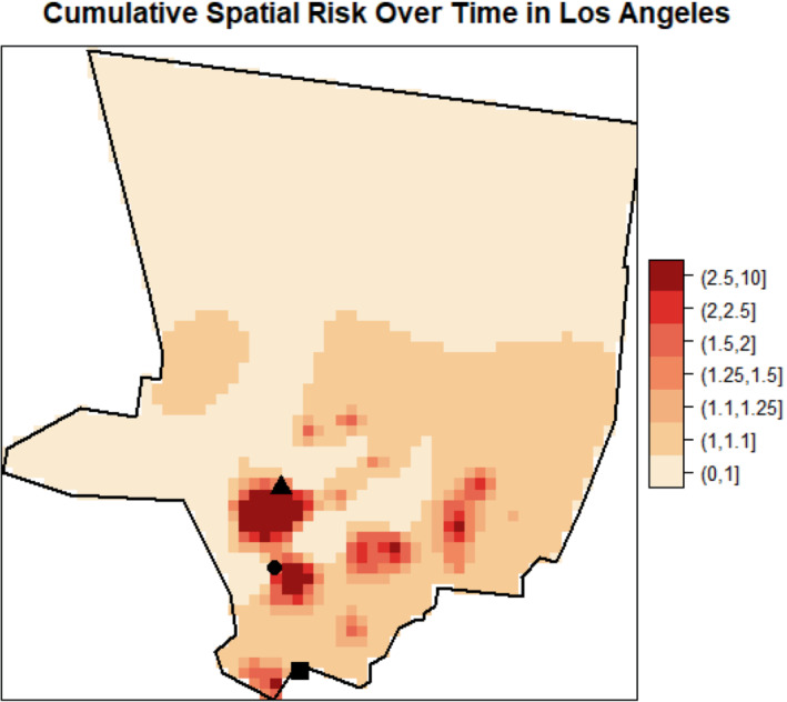
Estimated cumulative spatial odds ratios for non‐Hodgkin lymphoma in the Los Angeles study center. Hollywood (triangle), Inglewood (circle), and Long Beach (square) are marked on the map

FIGURE 4.

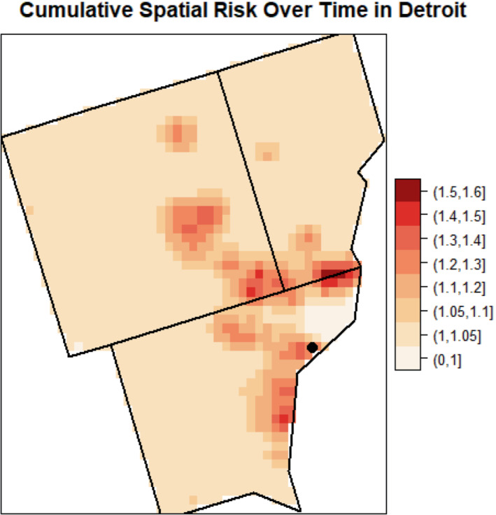
Estimated cumulative spatial odds ratios for non‐Hodgkin lymphoma in the Detroit study center. The Detroit city center (circle) is marked on the map

FIGURE 5.

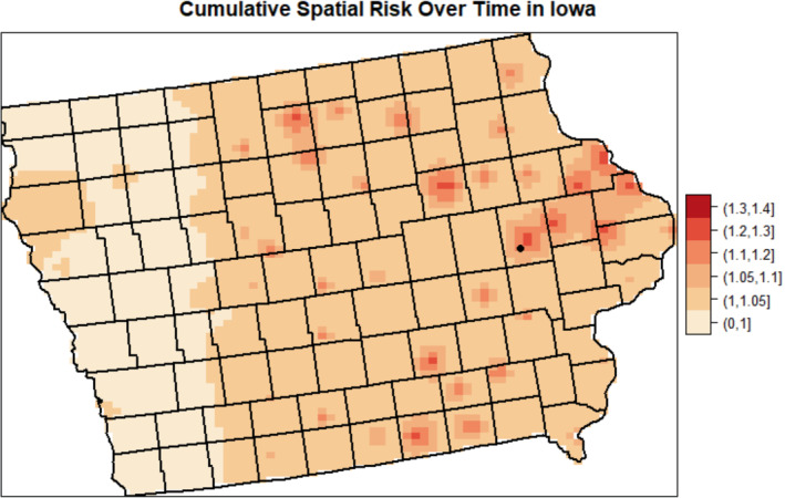
Estimated cumulative spatial odds ratios for non‐Hodgkin lymphoma in the Iowa study center. Cedar Rapids (circle) is marked on the map

FIGURE 6.

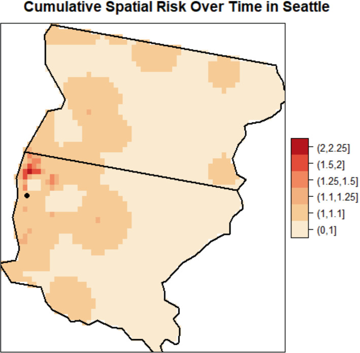
Estimated cumulative spatial odds ratios for non‐Hodgkin lymphoma in the Seattle study center. The Seattle city center is marked (circle) on the map

Regarding significance of the spatial risk estimates, the area of cumulative spatial risk in Los Angeles near West Hollywood and Beverly Hills is significantly elevated according to the exceedance probabilities (Figure 7). This area of significantly elevated risk is approximately 20 km². We calculated the number of case and control residential locations and the number of cases and controls in this area to help characterize the empirical risk over time. The empirical (observed) odds ratio was 4.15 based on case and control residential locations (54 and 13 locations, respectively), and 3.40 based on cases and controls (34 and 10 participants, respectively). There were no statistically significant areas of elevated risk in Detroit, Iowa, or Seattle.

FIGURE 7.

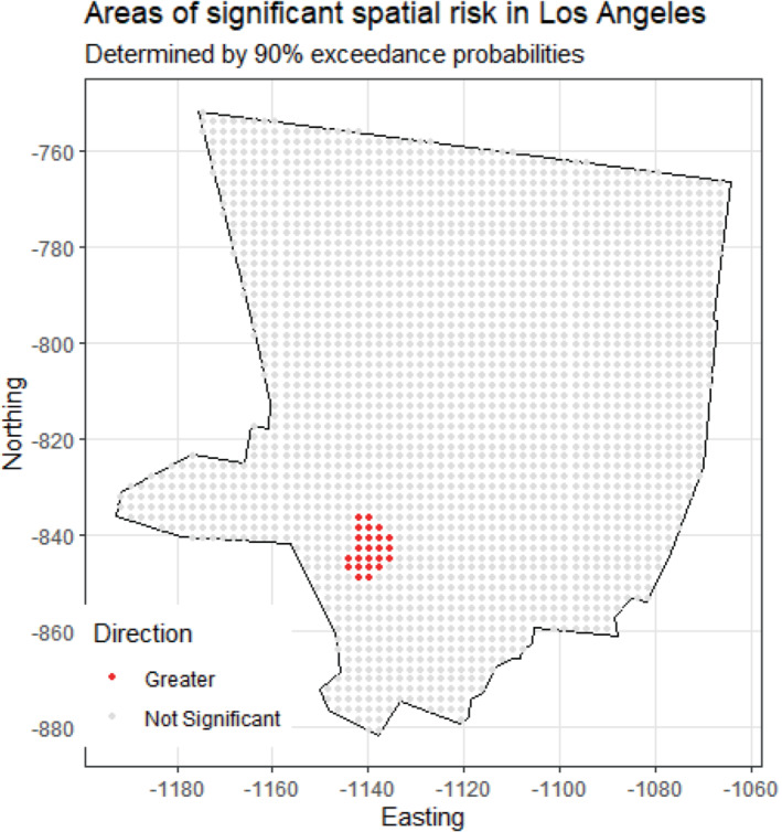
Areas of significantly elevated cumulative spatial risk for non‐Hodgkin lymphoma in the Los Angeles study center

4. DISCUSSION

In this article, we proposed the Bayesian index low‐rank kriging multiple membership model to simultaneously estimate the effects of groups of correlated exposures and estimate cumulative spatial risk over time within a study area. We designed the model for use in a case‐control study that measures many exposures and collects residential histories. We evaluated the performance of the model though a simulation study that included a wide variety of plausible scenarios that represent part of the environmental risk for an adverse health outcome. In particular, we varied the number of groups of exposures, the magnitude, and direction of health effects associated with each group index, and the correlation structure

and strength of components in a group index in a study region that contained a persistent zone of elevated spatial risk. In the simulation study, we found that the model was able to estimate the health effects of one or several groups of exposures precisely and with adequate coverage, demonstrated by averaging its performance over many simulated datasets. Particularly, the model was able to accurately estimate the health effects of a group index in the presence of high correlation among components of the index. Additionally, for almost every dataset in every scenario, the model correctly identified some portion of a zone of true elevated spatial risk.

We applied our model to the NCI‐SEER NHL study at four separate study centers across the United States: Detroit, Iowa, Los Angeles, and Seattle. We analyzed four groups of chemical exposures (PCBs, PAHs, and two groups of pesticides), used residential histories for study participants, and controlled for a set of demographic covariates in our models. In Iowa, we identified a significant and positive association between one index of pesticides and risk for NHL, where a one‐unit increase in the index corresponded to 1.5 times greater odds of NHL. The most important chemicals in this index were propoxur, gamma‐chlordane, and alpha‐chlordane, which collectively accounted for approximately two‐thirds of the total weight of the index. This finding supports that of a previous analysis of the NCI‐SEER NHL study, which used WQS regression to estimate the effect of one group of 27 chemical exposures for each NHL center. ⁵⁰ In that analysis, the index was positively and significantly associated with risk of NHL in Iowa. Additionally, propoxur had the highest weight in the index, and alpha‐chlordane and gamma‐chlordane were among the five most highly‐weighted chemicals. We also found a significant inverse association between another index of pesticides and risk for NHL in Iowa, where a one‐unit increase in the index corresponded to approximately five times smaller odds of NHL. In this index, the most highly weighted chemical was 2,4‐D. In the previous WQS analysis, the weight for 2,4‐D was less than 0.005, suggesting negligible contribution to the single index, which was positively associated with risk for NHL. ³⁹ Our model, with multiple group indices, each of which could vary in magnitude and direction with the outcome, allows for direct inference on the negative association between 2,4‐D and NHL in a group of negative‐association chemicals. This result is more informative than finding that 2,4‐D has effectively no weight in a positive‐association index for NHL. In the PCB index, congener 180 had the highest estimated weight at two centers (Detroit in Seattle). A previous logistic regression analysis of PCBs and other organochlorines measured in plasma found that PCB 180 had a significant association with NHL risk when comparing the highest versus lowest quartiles, as did other PCB congeners as well as furan congeners. ⁷ We note that PCBs are considered carcinogenic to humans (Group 1), and chlordane and 2,4‐D are considered possibly carcinogenic to humans (Group 2B) according to the most recent classifications from the International Agency for Research on Cancer working group. ⁵⁵

In Los Angeles, Detroit, and Seattle, we did not find any significant association between chemical indices and NHL. This finding provides more site‐specific conclusions regarding the chemical index‐NHL relationship than does a previous frequentist analysis of the NHL data that employed grouped WQS regression. ⁵¹ The previous analysis estimated overall mixture effects in one model and used the same data in the two steps of model fitting and validation to find significant positive associations between the PCB and pesticides index I and NHL and a significant negative association between the pesticides index II and NHL over the four combined study centers. ⁵¹ The significant findings from the previous study may have been from using a larger sample size in one model or possibly from overfitting due to not separating the data used for estimation and validation. In our analysis, we used only the data specific to a given study center in modeling mixture effects in that center due to the inclusion of the spatial risk component, which is site‐specific. Overall, our model allows more direct inference on the health effects of different chemical groups on NHL risk in different study centers by allowing group effects to vary in magnitude and direction in each center.

Regarding spatial risk over time, we identified a cluster of elevated spatial risk for NHL in Los Angeles, west of the city center. The cluster was approximately 20 km² and generally consisted of local spatial odds ratios of 2.5 for risk of NHL. A previous spatial analysis using generalized additive models (GAMs) and individual lag times prior to diagnosis and adjusted for a similar set of covariates (but not for 27 chemical exposures measured inside the home) found a similar cluster of elevated spatial risk for NHL in this region at a lag time of 20 years. ⁵⁴ Specifically, the GAM analysis fit models using residential locations at a set of individual lag times (at diagnosis, as well as 5, 10, 15, and 20 years before diagnosis), and the cluster in Los Angeles was only identified using residential locations 20 years before diagnosis. In our analysis, we used all of subjects' residential locations to estimate cumulative spatial risk in the study region, and by simultaneously estimating the health effects of groups of chemical exposures, and so in contrast to the GAM analysis, any resultant cluster of spatial risk from this model can be considered to exist above and beyond such chemical exposures. Overall, our model provides a more complete estimate of cumulative spatial risk through weighting study participants' residences by duration lived. The construction of our spatial risk component utilizes entire residential histories, not just locations at certain lag times, in order to use maximal information for estimation of unmeasured exposures for NHL risk.

Based on our findings, we believe that the Bayesian index LRK‐MMM can provide a powerful tool for researchers interested in a more comprehensive estimate of environmental risk. In reality, measured chemical mixtures and unmeasured environmental exposures over time act on individuals simultaneously, and our model is the first to estimate both components simultaneously in an integrated modeling framework. Additionally, situating the model in the Bayesian paradigm allows for utilization of the entire sample, incorporation of previous information through the prior distribution, and simultaneous estimation of the full posterior distribution of all parameters, which provides maximal information to perform inference on any parameter of interest. This represents an improvement upon traditional WQS approaches that require data splitting for the estimation and validation model steps. Another strength of the model we propose is its generality, because an analyst can adapt model components to their data. For example, while the outcome variable we used in our data application was case or control status, the outcome could be any type of variable, such as smoker/non‐smoker, received early screening test/did not screen, number of disease cases in a region, or more. Further, the group exposure indices need not be restricted to chemical groups, but could for example be socio‐economic indices, with the groups measured at different time points or different spatial scales. Finally, through low‐rank kriging, our model provides a computationally efficient means to estimate cumulative spatial risk using point locations for subjects.

While our model has several strengths, some limitations may motivate future research. First, while the Bayesian index LRK‐MMM is designed to estimate spatial risk that is cumulative, it does not identify the specific timing of historic elevated risk. For example, an analysis may seek to identify if a particular time period (eg, calendar year) had relatively more explanatory power in spatial risk than other years in residential histories, potentially due to some acute event. Second, while our data application controlled for a temporally‐fixed set of covariates and used measurements of chemical mixtures that were collected at one time point, it is possible that in other studies the covariates or chemical exposures could be time‐varying, which represents an opportunity to extend the model given the necessary time‐varying data components. Finally, we note that other methods beyond LRK exist that estimate spatial risk in a computationally efficient manner. For example, fixed rank kriging (FRK) enables efficient spatial prediction for very large datasets through the use of a flexible class of non‐stationary covariance functions that use a fixed number of basis functions. ⁵⁶

In conclusion, our Bayesian index LRK‐MMM is a novel way to estimate risk of two broad components of risk analysis, measured, and unmeasured environmental exposures. The method accommodates groups of measured exposures and residential histories for study participants and can be adapted to a wide range of outcome variables and exposures, making it a flexible and powerful choice for public health practitioners. Conclusions drawn from the model, such as health effects estimated for a group of exposures, important components within exposure groups, and areas of significantly elevated spatial risk, beget natural public health responses, such as remediation efforts among highly‐exposed individuals, programs to reduce future exposures to important and harmful exposures, and epidemiologic investigations focused on elucidating causes of persistent elevated spatial risk. For example, a reasonable next step given the findings of our analysis of the NHL data would be to investigate potential sources of the cluster of significantly elevated risk of NHL in Los Angeles. As such, the Bayesian index LRK‐MMM represents another step in implementing the ideal of the exposome into environmental risk analyzes.

FUNDING INFORMATION

Research reported in this publication was supported by the National Cancer Institute of the National Institutes of Health under Award Number U01CA259376. The content is solely the responsibility of the authors and does not necessarily represent the official views of the National Institutes of Health.

Supporting information

Appendix S1 Supporting Information

Boyle J, Ward MH, Cerhan JR, Rothman N, Wheeler DC. Estimating mixture effects and cumulative spatial risk over time simultaneously using a Bayesian index low‐rank kriging multiple membership model. Statistics in Medicine. 2022;41(29):5679‐5697. doi: 10.1002/sim.9587

DATA AVAILABILITY STATEMENT

The data that support the findings of this study are available on request from the author Dr. Nat Rothman. The data are not publicly available due to privacy or ethical restrictions.

REFERENCES

- 1. Wild CP. Complementing the genome with an “exposome”: the outstanding challenge of environmental exposure measurement in molecular epidemiology. Cancer Epidemiol Prev Biomarkers. 2005;14(8):1847‐1850. [DOI] [PubMed] [Google Scholar]
- 2. DeBord DG, Carreón T, Lentz TJ, Middendorf PJ, Hoover MD, Schulte PA. Use of the “exposome” in the practice of epidemiology: a primer on‐omic technologies. Am J Epidemiol. 2016;184(4):302‐314. [DOI] [PMC free article] [PubMed] [Google Scholar]
- 3. de Vuijst E, van Ham M, Kleinhans R. A life course approach to understanding neighbourhood effects. IZA Discussion Paper #10276; 2016.
- 4. Wild CP, Turner PC. The toxicology of aflatoxins as a basis for public health decisions. Mutagenesis. 2002;17(6):471‐481. [DOI] [PubMed] [Google Scholar]
- 5. Colt JS, Severson RK, Lubin J, et al. Organochlorines in carpet dust and non‐Hodgkin lymphoma. Epidemiology. 2005;16:516‐525. [DOI] [PubMed] [Google Scholar]
- 6. Brown LM, Blair A, Gibson R, et al. Pesticide exposures and other agricultural risk factors for leukemia among men in Iowa and Minnesota. Cancer Res. 1990;50(20):6585‐6591. [PubMed] [Google Scholar]
- 7. de Roos AJ, Hartge P, Lubin JH, et al. Persistent organochlorine chemicals in plasma and risk of non‐Hodgkin's lymphoma. Cancer Res. 2005;65(23):11214‐11226. [DOI] [PubMed] [Google Scholar]
- 8. Ward MH, Colt JS, Metayer C, et al. Residential exposure to polychlorinated biphenyls and organochlorine pesticides and risk of childhood leukemia. Environ Health Perspect. 2009;117(6):1007‐1013. [DOI] [PMC free article] [PubMed] [Google Scholar]
- 9. Purdue MP, Hoppin JA, Blair A, Dosemeci M, Alavanja MCR. Occupational exposure to organochlorine insecticides and cancer incidence in the agricultural health study. Int J Cancer. 2007;120(3):642‐649. [DOI] [PMC free article] [PubMed] [Google Scholar]
- 10. Reuben SH. Reducing Environmental Cancer Risk: What we Can Do Now. Darby: DIANE Publishing; 2010. [Google Scholar]
- 11. Li Z, Christensen GM, Lah JJ, et al. Neighborhood characteristics as confounders and effect modifiers for the association between air pollution exposure and subjective cognitive functioning. Environ Res. 2022;212:113221. [DOI] [PMC free article] [PubMed] [Google Scholar]
- 12. Wheeler DC, Boyle J, Barsell DJ, et al. Tobacco retail outlets, neighborhood deprivation and the risk of prenatal smoke exposure. Nicotine Tob Res. 2022. [DOI] [PMC free article] [PubMed] [Google Scholar]
- 13. Lian M, Madden PA, Lynskey MT, et al. Geographic variation in maternal smoking during pregnancy in the Missouri adolescent female twin study (MOAFTS). PLoS One. 2016;11(4):e0153930. doi: 10.1371/journal.pone.0153930 [DOI] [PMC free article] [PubMed] [Google Scholar]
- 14. Kim SS, Meeker JD, Keil AP, et al. Exposure to 17 trace metals in pregnancy and associations with urinary oxidative stress biomarkers. Environ Res. 2019;179:108854. [DOI] [PMC free article] [PubMed] [Google Scholar]
- 15. Keil AP, Buckley JP, O'Brien KM, Ferguson KK, Zhao S, White AJ. A quantile‐based g‐computation approach to addressing the effects of exposure mixtures. Environ Health Perspect. 2020;128(4):47004. [DOI] [PMC free article] [PubMed] [Google Scholar]
- 16. Wheeler DC, Rustom S, Carli M, Whitehead TP, Ward MH, Metayer C. Bayesian group index regression for modeling chemical mixtures and cancer risk. Int J Environ Res Public Health. 2021;18(7):3486. [DOI] [PMC free article] [PubMed] [Google Scholar]
- 17. Vieira V, Webster T, Weinberg J, Aschengrau A. Spatial analysis of bladder, kidney, and pancreatic cancer on upper Cape Cod: an application of generalized additive models to case‐control data. Environ Health. 2009;8(1):1‐13. [DOI] [PMC free article] [PubMed] [Google Scholar]
- 18. Vieira VM, Webster TF, Weinberg JM, Aschengrau A. Spatial‐temporal analysis of breast cancer in upper Cape Cod, Massachusetts. Int J Health Geogr. 2008;7(1):1‐12. [DOI] [PMC free article] [PubMed] [Google Scholar]
- 19. Jacquez GM, Kaufmann A, Meliker J, Goovaerts P, AvRuskin G, Nriagu J. Global, local and focused geographic clustering for case‐control data with residential histories. Environ Health. 2005;4(1):4. doi: 10.1186/1476-069X-4-4 [DOI] [PMC free article] [PubMed] [Google Scholar]
- 20. Wheeler DC, Waller LA, Cozen W, Ward MH. Spatial–temporal analysis of non‐Hodgkin lymphoma risk using multiple residential locations. Spat Spatiotemporal Epidemiol. 2012;3(2):163‐171. [DOI] [PMC free article] [PubMed] [Google Scholar]
- 21. Boyle J, Ward MH, Koutros S, et al. Estimating cumulative spatial risk over time with low‐rank kriging multiple membership models. Stat Med. 2022. [DOI] [PMC free article] [PubMed] [Google Scholar]
- 22. Petrof O, Neyens T, Nuyts V, Nackaerts K, Nemery B, Faes C. On the impact of residential history in the spatial analysis of diseases with a long latency period: a study of mesothelioma in Belgium. Stat Med. 2020;39(26):3840‐3866. [DOI] [PubMed] [Google Scholar]
- 23. Nychka DW, Bailey BA, Ellner SP, Haaland PD, O'Connell MA. FUNFITS data analysis and statistical tools for estimating functions; North Carolina State University; 1996.
- 24. Furrer R, Nychka D, Sain S, Nychka MD. Tools for spatial data; 2012.
- 25. Wheeler DC, Wang A. Assessment of residential history generation using a public‐record database. Int J Environ Res Public Health. 2015;12(9):11670‐11682. [DOI] [PMC free article] [PubMed] [Google Scholar]
- 26. Meliker JR, Slotnick MJ, AvRuskin GA, et al. Lifetime exposure to arsenic in drinking water and bladder cancer: a population‐based case‐control study in Michigan, USA. Cancer Causes Control. 2010;21(5):745‐757. [DOI] [PMC free article] [PubMed] [Google Scholar]
- 27. Christensen KLY, Carrico CK, Sanyal AJ, Gennings C. Multiple classes of environmental chemicals are associated with liver disease: NHANES 2003–2004. Int J Hyg Environ Health. 2013;216(6):703‐709. [DOI] [PMC free article] [PubMed] [Google Scholar]
- 28. Hargarten PM, Wheeler DC. Accounting for the uncertainty due to chemicals below the detection limit in mixture analysis. Environ Res. 2020;186:109466. [DOI] [PubMed] [Google Scholar]
- 29. Shaddick G, Zidek JV. A case study in preferential sampling: long term monitoring of air pollution in the UK. Spat Stat. 2014;9:51‐65. [Google Scholar]
- 30. Diggle PJ, Tawn JA, Moyeed RA. Model‐based geostatistics. J R Stat Soc Ser C Appl Stat. 1998;47(3):299‐350. [Google Scholar]
- 31. Johnson ME, Moore LM, Ylvisaker D. Minimax and maximin distance designs. J Stat Plan Inference. 1990;26(2):131‐148. [Google Scholar]
- 32. Wang H, Ranalli MG. Low‐rank smoothing splines on complicated domains. Biometrics. 2007;63(1):209‐217. [DOI] [PubMed] [Google Scholar]
- 33. Roy J, Stewart WF. Estimation of age‐specific incidence rates from cross‐sectional survey data. Stat Med. 2010;29(5):588‐596. [DOI] [PubMed] [Google Scholar]
- 34. Wheeler DC, Calder CA. Sociospatial epidemiology: residential history analysis. In: Andrew BL, Sudipto B, Robert PH, Maria DU, eds. Handbook of Spatial Epidemiology. Boca Raton: Chapman and Hall/CRC; 2016:627‐648. [Google Scholar]
- 35. Crainiceanu CM, Diggle PJ, Rowlingson B. Bivariate binomial spatial modeling of Loa loa prevalence in tropical Africa. J Am Stat Assoc. 2008;103(481):21‐37. [Google Scholar]
- 36. Boyle J, Wheeler DC. Knot selection for low‐rank kriging models of spatial risk in case‐control studies. Spat Spatiotemporal Epidemiol. 2022;41:100483. [DOI] [PMC free article] [PubMed] [Google Scholar]
- 37. Teitz MB, Bart P. Heuristic methods for estimating the generalized vertex median of a weighted graph. Oper Res. 1968;16(5):955‐961. [Google Scholar]
- 38. Owen SH, Daskin MS. Strategic facility location: a review. Eur J Oper Res. 1998;111(3):423‐447. [Google Scholar]
- 39. Czarnota J, Wheeler DC, Gennings C. Evaluating geographically weighted regression models for environmental chemical risk analysis. Cancer Inform. 2015;14:117‐127. [DOI] [PMC free article] [PubMed] [Google Scholar]
- 40. Colt JS, Lubin J, Camann D, et al. Comparison of pesticide levels in carpet dust and self‐reported pest treatment practices in four US sites. J Expo Sci Environ Epidemiol. 2004;14(1):74‐83. [DOI] [PubMed] [Google Scholar]
- 41. Lubin JH, Colt JS, Camann D, et al. Epidemiologic evaluation of measurement data in the presence of detection limits. Environ Health Perspect. 2004;112(17):1691‐1696. [DOI] [PMC free article] [PubMed] [Google Scholar]
- 42. Plummer M. JAGS: A program for analysis of Bayesian graphical models using Gibbs sampling. Proceedings of the 3rd International Workshop on Distributed Statistical Computing; 2003:1‐10.
- 43. R Core Team and Others . R: A language and environment for statistical computing; 2021.
- 44. Gelman A, Rubin DB. Inference from iterative simulation using multiple sequences. Stat Sci. 1992;7(4):457‐472. [Google Scholar]
- 45. Plummer M, Best N, Cowles K, Vines K. CODA: convergence diagnosis and output analysis for MCMC. R News. 2006;6(1):7‐11. https://www.r‐project.org/doc/Rnews/Rnews_2006‐1.pdf [Google Scholar]
- 46. Richardson S, Thomson A, Best N, Elliott P. Interpreting posterior relative risk estimates in disease‐mapping studies. Environ Health Perspect. 2004;112(9):1016‐1025. [DOI] [PMC free article] [PubMed] [Google Scholar]
- 47. Chatterjee N, Hartge P, Cerhan JR, et al. Risk of non‐Hodgkin's lymphoma and family history of lymphatic, hematologic, and other cancers. Cancer Epidemiol Prev Biomarkers. 2004;13(9):1415‐1421. [PubMed] [Google Scholar]
- 48. Morton LM, Wang SS, Cozen W, et al. Etiologic heterogeneity among non‐Hodgkin lymphoma subtypes. Blood. 2008;112(13):5150‐5160. [DOI] [PMC free article] [PubMed] [Google Scholar]
- 49. ESRI . ArcView 3.2.
- 50. Czarnota J, Gennings C, Colt JS, et al. Analysis of environmental chemical mixtures and non‐Hodgkin lymphoma risk in the NCI‐SEER NHL study. Environ Health Perspect. 2015;123(10):965‐970. [DOI] [PMC free article] [PubMed] [Google Scholar]
- 51. Wheeler D, Czarnota J. Modeling chemical mixture effects with grouped weighted quantile sum regression. ISEE Conference Abstracts; 2016.
- 52. Spiegelhalter DJ, Best NG, Carlin BP, van der Linde A. Bayesian measures of model complexity and fit. J R Stat Soc Series B Stat Methodol. 2002;64(4):583‐639. [Google Scholar]
- 53. Lawson AB, Banerjee S, Haining RP, Ugarte MD. Handbook of Spatial Epidemiology. Boca Raton: CRC press; 2016. [Google Scholar]
- 54. Wheeler DC, de Roos AJ, Cerhan JR, et al. Spatial‐temporal analysis of non‐Hodgkin lymphoma in the NCI‐SEER NHL case‐control study. Environ Health. 2011;10(1):1‐13. [DOI] [PMC free article] [PubMed] [Google Scholar]
- 55. IARC . Agents Classified by the IARC Monographs, Volumes 1–129. Lyon, France: International Agency for Research on Cancer. 2021. Accessed May 19, 2022. http://monographs.iarc.fr/ENG/Classification/index.php [Google Scholar]
- 56. Cressie N, Johannesson G. Fixed rank kriging for very large spatial data sets. J R Stat Soc Ser B. 2008;70(1):209‐226. [Google Scholar]
Associated Data
This section collects any data citations, data availability statements, or supplementary materials included in this article.
Supplementary Materials