High-quality PET image synthesis from ultra-low-dose PET/MRI using bi-task deep learning

Abstract

Background

Lowering the dose for positron emission tomography (PET) imaging reduces patients’ radiation burden but decreases the image quality by increasing noise and reducing imaging detail and quantifications. This paper introduces a method for acquiring high-quality PET images from an ultra-low-dose state to achieve both high-quality images and a low radiation burden.

Methods

We developed a two-task-based end-to-end generative adversarial network, named bi-c-GAN, that incorporated the advantages of PET and magnetic resonance imaging (MRI) modalities to synthesize high-quality PET images from an ultra-low-dose input. Moreover, a combined loss, including the mean absolute error, structural loss, and bias loss, was created to improve the trained model’s performance. Real integrated PET/MRI data from 67 patients’ axial heads (each with 161 slices) were used for training and validation purposes. Synthesized images were quantified by the peak signal-to-noise ratio (PSNR), normalized mean square error (NMSE), structural similarity (SSIM), and contrast noise ratio (CNR). The improvement ratios of these four selected quantitative metrics were used to compare the images produced by bi-c-GAN with other methods.

Results

In the four-fold cross-validation, the proposed bi-c-GAN outperformed the other three selected methods (U-net, c-GAN, and multiple input c-GAN). With the bi-c-GAN, in a 5% low-dose PET, the image quality was higher than that of the other three methods by at least 6.7% in the PSNR, 0.6% in the SSIM, 1.3% in the NMSE, and 8% in the CNR. In the hold-out validation, bi-c-GAN improved the image quality compared to U-net and c-GAN in both 2.5% and 10% low-dose PET. For example, the PSNR using bi-C-GAN was at least 4.46% in the 2.5% low-dose PET and at most 14.88% in the 10% low-dose PET. Visual examples also showed a higher quality of images generated from the proposed method, demonstrating the denoising and improving ability of bi-c-GAN.

Conclusions

By taking advantage of integrated PET/MR images and multitask deep learning (MDL), the proposed bi-c-GAN can efficiently improve the image quality of ultra-low-dose PET and reduce radiation exposure.

Introduction

The role positron emission tomography (PET) plays in modern clinical/preclinical medicine is extraordinary. Patients who undertake PET for treatment are injected with a large dose of radioactive tracer into tissues or organs before scanning. This process generates radiation exposure, which will inevitably be uncomfortable or harmful to patients, especially in patients who need multiple examinations or pediatric patients with a higher lifetime risk for developing cancer. Although lowering the dose of radioactive tracer can reduce radiation exposure, it also yields increased noise, artifacts, and a lack of imaging details (1). The contradiction between lowering radiation exposure and improving imaging quality has attracted much research interest in this area, including using more sophisticated facilities or advanced signal processing algorithms. Manufacturers have tried to improve the sensitivity of PET scanners by using higher-performance detectors that are straightforward but expensive (2). Moreover, once the scanners are established for a PET system, there is no room for data quality optimization (3). For a long time, algorithm-based techniques have focused on PET reconstruction from sinogram data (4-7) or traditional patch-based learning methods (8-10), which involve limitations such as high demand for data, high time consumption, or poor output quality (11-13). Deep learning algorithm methods, especially the encoder-decoder structure, with its powerful data-driven capabilities between image datasets, can develop an image transferring model with high fitness and efficiency (14-16). Recently developed integrated PET/magnetic resonance imaging (MRI) scanners enable the simultaneous acquisition of structural and functional information without extra radiation exposure, which gives more information and the potential for deep learning-based methods. Multitask deep learning (MDL) can improve generalizability by using the domain information contained in the training signals of related tasks as an inductive bias (17). Implementation of MDL has led to successes in fields from natural language processing to computer vision (18). To the best of our knowledge, MDL has not been used in a medical image synthesizing task such as high-quality PET synthesis. Given the above, this paper attempts an MDL-based method and treats MRI as a related source in helping to synthesize high-quality PET images from its ultra-low-dose modality.

Related works

Improving ultra-low-dose PET image quality by mapping these images to the ground truth, full-dose PET images is a pixel-level prediction task for which convolutional neural networks (CNNs) have been widely used (19). Earlier, Gong et al. (20) trained a deep CNN from low-dose PET images (20% of the full dose) to full-dose PET images using simulated data and fine-tuned it with real data. Later, Wang et al. (21) performed similar work by improving whole-body PET quality using a CNN with corresponding MR images. Previous works also showed the strength of CNN with a U-net structure in synthesizing high-quality PET images (22-24). There is a tendency for CNNs to produce blurry results (25), but generative adversarial networks (GANs) may solve this by using a structural loss (26). Given this, Wang et al. (27) trained a GAN to improve the quality of low-dose PET images (25% of the full dose). Later, Isola (28) showed that a conditional GAN (c-GAN) with a conditional input and a skip connection, if trained using a combination of L1 loss and structured loss, could achieve an advantage in image–image translation tasks, which was then adopted by Wang (29). A c-GAN structure requires a conditional input which was realized by treating low-dose PET as conditional inputs (30,31). Many others have also found the advantage of anatomical information in PET denoising. Cui (32) took advantage of patients’ prior MR/computed tomography (CT) images and treated them as conditional inputs for a U-net to restore low-dose PET images. Considering input MR can influence the results of output PET, Onishi et al. (33) only treated MR as a prior guide when using a deep decoder network to synthesize PET from random noise. However, low-dose PET was not treated as an input of the network until recently. Chen (23,34) used a simple U-net and treated both low-dose PET and multiple MRI as conditional inputs to improve the quality of low-dose PET images.

Unlike in our study, the deep learning methods above are based on single-task learning (STL). We used a two-task based MDL method called bi-task. In bi-task, MRI is treated as an additional task (18) rather than additional channels in one task (21,23,27,34). Therefore, the impact of MR as input can be avoided while at the same time maintaining its effect of guidance. An MDL works because the regularization induced by requiring an algorithm to perform well on a related task can be superior to ordinary regularization, which prevents overfitting by uniformly penalizing all complexity (35,36). A problem with MDL is negative transfer, which should be avoided because it leads to performance degradation (37). An instance when MDL may be particularly helpful is when the tasks are similar and are generally slightly under-sampled (17). For these two reasons, MDL fit our case well. First, the generation of high-quality PET images from MRI modalities or low-dose PET images has the same target. Second, the slices used to train the network are often limited because of the difficulty in obtaining real patient images in large numbers. Kuga’s (38) MDL structure used for multi-input, multi-target scene recognition is similar to our bi-task structure. One difference is that bi-task is multi-input single-target. Previous methods for multi-input single-target structures are building a multi-encoder and a single-decoder (39). A weakness of the multi-encoder single-decoder structure is that straightforward concatenation of extracted features from different encoders to one decoder often results in inaccurate estimation results (38). To avoid this weakness, we created two decoders by directing them to two targets (namely, the target for the first input and the target for the second input) to construct a multi-input multi-target structure.

Our contributions

This paper tries to improve the quality of ultra-low-dose PET axial head images by training a bi-task network with ultra-low-dose PET images (5% of the full dose) and integrating T1-weighted MRI images for the input and full-dose PET images as the ground truth labels. The strengths of conditional input, GAN, and skip connection were added to the bi-task. The combined structure was called bi-c-GAN. A combined loss, including Euclidean distance, structural loss, and bias loss, was developed and used in the training stage to fully extract information from three datasets (the full-dose PET image dataset, ultra-low-dose PET image dataset, and integrated MRI dataset). This paper’s main innovations and contributions are two-fold: (I) the bi-c-GAN network and its combined loss function were created, and the model was trained successfully using real patients’ data, which meant that the effect of each contributing part was analyzed specifically; (II) the general effect of the proposed bi-c-GAN in improving low-dose PET images’ quality was validated. Compared with U-net, c-GAN, and M-c-GAN (multiple conditional inputs of c-GAN treating MRI as an additional channel), the proposed bi-c-GAN achieved better performances in selected quantitative indexes. We present the following article in accordance with the MDAR reporting checklist (available at https://qims.amegroups.com/article/view/10.21037/qims-22-116/rc).

Methods

Bi-task structure

The basic bi-task structure was inspired by the work of Kuga et al. (38), with some changes made according to our application. The mechanism of this kind of MDL structure is as follows. An encoder is built for each input, and a shared latent representation layer follows each encoder. The latent representations are shared because the output from each latent representation acts as the input of each task’s decoder; in other words, each latent representation followed by their corresponding encoders will correspond to a task’s decoder. In the case of two-input/two-target, four encoder/decoder pairs are used for training. As shown in Figure 1, our case included two inputs, namely low-dose PET (x_LP) and T1-weighted MRI (x_T1), and two targets, namely high-quality synthesized PET images translating from low-dose PET images (y_LP) and high-quality synthesized PET images translating from T1-weighted MRI images (y_T1).

Figure 1.

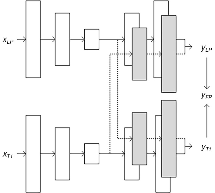
Illustration of a bi-task structure. The structure includes an input pair (x_LP,x_T1), an output pair (y_LP,y_T1), and four encoder-decoder pairs with each encoder’s output passed to both targets’ decoders. In this study, output pairs have the same value of y_FP.

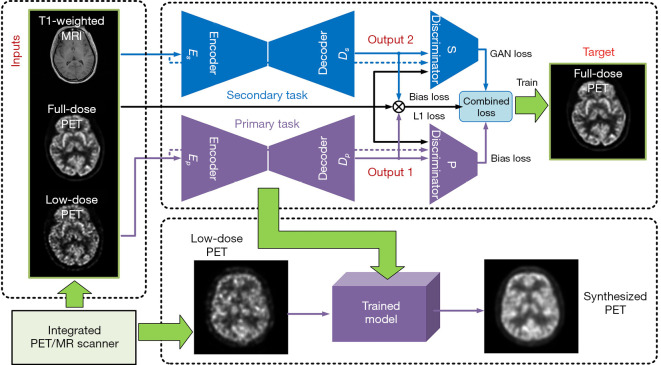
Given that the MRI is used to assist the PET-synthesizing process, we called the task conditioned on low-dose PET images the primary task and the task conditioned on the MRI image the secondary task. Both tasks worked in parallel and crossed each other. x_LP was the input of the primary task and x_T1 represented the input of the secondary task. Inputs x_LP and x_T1 were directly followed by their corresponding encoders E_p (·) and E_s (·). E_p (x_LP) and E_s (x_T1), which comprised the layer of shared latent representation, as the outputs of the two encoders. The representation layer was completely shared by all the decoders, which meant that the output of each encoder was fed into all the decoders (as shown in Figure 1, the dash line crossing each task); therefore, there were four encoder/decoder pairs given: an input pair (x_LP, x_T1) and a target pair (y_LP, y_T1). D (·) was the function of the decoder, and was the synthesized output of each decoder. Then, we obtained the following:

$$\{\begin{array}{c}{\widehat{y}}_{x_{LP}\to y_{LP}}=D_{x_{LP}\sim y_{LP}}\left[E_P\left(x_{LP}\right)\right]\\ {\widehat{y}}_{x_{LP}\to y_{T1}}=D_{x_{LP}\sim y_{T1}}\left[E_P\left(x_{LP}\right)\right]\\ {\widehat{y}}_{x_{T1}\to y_{LP}}=D_{x_{T1}\sim y_{LP}}\left[E_a\left(x_{T1}\right)\right]\\ {\widehat{y}}_{x_{T1}\to y_{T1}}=D_{x_{T1}\sim y_{T1}}\left[E_a\left(x_{T1}\right)\right]\end{array}$$ [1]

where ${\widehat{y}}_{x\to y}$ represents an encoder-decoder’s synthesized result from an input x to a target y and the corresponding decoder’s function is denoted by D_x~y. Specifically, both of the primary task and secondary task’s targets aimed to synthesize a high-quality PET image as similar as a full-dose PET image, denoted by y_FP as shown in Figure 1, as much as possible, which meant that the ${\widehat{y}}_{x\to y}$ of the above Eq. [1] yielded equal values when the corresponding decoders reached their final formation after a training process in Eq. [2]:

$$\{\begin{array}{c}\underset{D\to D_{best}}{\lim }\left({\widehat{y}}_{x_{LP}\to y_{LP}}\right)=\underset{D\to D_{best}}{\lim }\left({\widehat{y}}_{x_{T1}\to y_{LP}}\right)=y_{LP}\\ \underset{D\to D_{best}}{\lim }\left({\widehat{y}}_{x_{LP}\to y_{T1}}\right)=\underset{D\to D_{best}}{\lim }\left({\widehat{y}}_{x_{T1}\to y_{T1}}\right)=y_{T1}\\ y_{LP}=y_{T1}=y_{FP}\end{array}$$ [2]

Note that, with the same input and target, the training processes of Eq. [1]’s decoders $D_{x_{LP}\sim y_{LP}}$ and $D_{x_{LP}\sim y_{T1}}$ are very similar, as are $D_{x_{T1}\sim y_{LP}}$ and $D_{x_{T1}\sim y_{T1}}$. For simplicity, we only retained $D_{x_{LP}\sim y_{LP}}$ and $D_{x_{T1}\sim y_{T1}}$ in our final model.

After simplification, two encoder-decoder pairs remained in our network, of which E_p (x_LP) and belonged to the primary task, E_s (x_T1) and belonged to the secondary task, as E_p, D_p, E_s, and D_s, respectively (Figure 2). In Figure 2, two discriminators for each task were added to the bi-task structure, which was then called bi-c-GAN. The primary task had its discriminator and encoder’s inputs conditioned on the low-dose PET image; the decoder’s output aligned to the ground truth full-dose PET image. The secondary task had its discriminator and encoder’s inputs conditioned on the MRI image; the decoder’s output aligned to the same ground truth full-dose PET image from the primary task. The combined loss was made up of both tasks’ mean absolute error and structural losses, in which the secondary task’s losses acted as the bias loss. The combined loss was used as the objective function to train and optimize the entire model.

Figure 2.

Illustration of the bi-c-GAN structure and the procedure of producing synthesized PET images. The main structure of bi-c-GAN and the training process are presented in the upper dotted block. The left dotted block shows the training pairs, which act as the inputs of the right network. The lower dotted block represents validating and testing stage in which the trained model is based on primary task’s generator. When testing by delivering the lose-dose PET images to the trained model, it will come out as synthesized PET images. c-GAN, conditional-generative adversarial network; PET, positron emission tomography; MRI, magnetic resonance imaging.

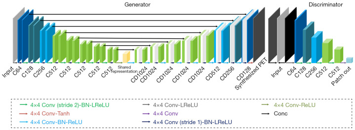
The generator and discriminator used in Figure 2 are shown in detail in Figure 3. They are composed of several basic blocks comprising convolutions (4×4 filters), batch normalization, dropout, and activation (rectified linear unit) layers. There are eight of the above basic blocks in the structures of the encoders and decoders, as shown in Figure 3. In the encoder part, we achieved down-sampling using strided convolution operations with a stride of 2. Because of skip connection, the last layer of each block in the encoder layers was concatenated with those in the decoder layers. In the output layer, the tanh activation function was used. The discriminator was mainly a 70×70 patch GAN in which five of the above basic blocks were included (26).

Figure 3.

Details of the model’s generator and discriminator. The different colored arrows in the lower block represent different kinds of computing methods as specified in the top, in which ‘Conv’ denotes the convolution operation, ‘BN’ denotes batch normalization, ‘ReLU’ denotes the rectified linear unit activation function, ‘LReLU’ denotes Leaky ReLU, and ‘Conc’ denotes the concatenation operation. Boxes represent tensors. Under each box, Ck denotes a convolution-like layer with k filters, and CDk denotes a convolution-like layer with a dropout rate of 50% with k filters.

Objective function

Given a batch of paired low-dose PET images and T1-weighted MRI images as inputs of our proposed model, we minimized the distance and the structural and bias losses between the synthesized image and the corresponding ground truth full-dose PET image. Here, we selected the L1 loss (l_L1) as the distance measure, as suggested by Isola et al. (28), and used GAN loss (l_GAN), which are patches out of the discriminator, as the structural loss. The bias loss (l_bias) came from the secondary task’s L1 and GAN losses. We defined the combined loss as the sum of the above losses. The gradients for the whole network were computed based on the combined loss by backpropagation. The combined loss was used for both tasks’ training processes.

Each discriminator provided structural loss for its corresponding task. A discriminator is an adversarial network that aims to distinguish the primary generator’s distribution from the labels. The primary generator’s output conditioned on an input x is denoted by G (x|θ_g), where G is the mapping from x to the synthesized output and θ_g is the parameter of G. The discriminator’s output conditioned on an input x and label y is denoted by D (x,y|θ_d), where D is the mapping and θ_d is the parameter of D. Combining G and D, a GAN is created by optimizing min_G max_D V (D,G), where V is the value function. The object of our GAN conditioned on x can be expressed as follows:

$${ℒ}_{cGAN}\left(G,D\right)={\mathbb{E}}_{x,y}\left[\log D\left(x,y\right)\right]+{\mathbb{E}}_x\left[\log \left(1-D\left(x,G\left(x\right)\right)\right)\right]$$ [3]

Both generators must fulfill the needs of approaching the ground truth by an L1 loss, in which that of the primary generator G_p is:

$${ℒ}_{L1}\left(G_p\right)={\mathbb{E}}_{x,y}\left[{\Vert y-G_p\left(x\right)\Vert }_1\right]$$ [4]

and that of the secondary generator G_s is:

$${ℒ}_{L1}\left(G_s\right)={\mathbb{E}}_{x,y}\left[{\Vert y-G_s\left(x\right)\Vert }_1\right]$$ [5]

The secondary task served as an inductive bias (17) that contributed all its losses as the bias loss; then, our final objective function was defined as follows:

$$\begin{array}{l}ℒ\left(G,cGAN\right)={\lambda }_p\left[{\lambda }_1{ℒ}_{L1}\left(G_p\right)+{\lambda }_2{ℒ}_{cGAN}\left(G_p,D_p\right)\right]\\ +{\lambda }_s\left[{\lambda }_3{ℒ}_{L1}\left(G_s\right)+{\lambda }_4{ℒ}_{cGAN}\left(G_s,D_s\right)\right]\end{array}$$ [6]

where λ₁ and λ₂ are weights of the primary network’s L1 loss and GAN loss, respectively; λ₃ and λ₄ are weights of the secondary network’s L1 loss and GAN loss, respectively; λ_p is the weight of the main loss; and λ_s is the weight of the bias loss.

Our study was conducted in accordance with the Declaration of Helsinki (as revised in 2013). Ethical approval (Sun Yat-sen University Cancer Center Guangzhou, China) was obtained, and the requirement for informed consent was waived for this retrospective analysis.

Experiment

Data acquisition and experiment settings

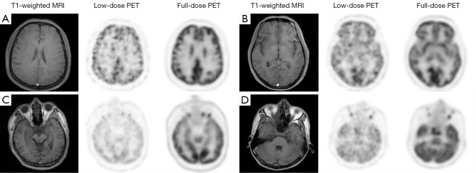
Real data from the axial head slices of 67 patients were used in our paper. Patients (both healthy and unhealthy cases) were between 22 and 73 years old (47±11 years old), of which 30% were female. The acquisition dates were from July 2020 to December 2020. The T1-weighted MRI and PET data were simultaneously acquired on an integrated 3.0T PET/MRI scanner (uPMR 790 PET/MR; United Imaging, Houston, TX, USA). Samples were acquired from patients 70.6±8.5 minutes after injection of 18F-fluorodeoxyglucose (FDG) (224.4±49.9 MBq), and FDG was administered intravenously after fasting for at least 6 h. All PET scans were reconstructed with the time-of-flight ordered-subset expectation maximization (OSEM) algorithm (20 subsets, 2 iterations, image matrix size of 192×192, voxel size of 3.125×3.125×2 mm³, and a 3 mm post-reconstruction image-space Gaussian filter). A full acquisition time of 10 minutes’ results was used for the ground truth full-dose PET image. Low-dose PET images were created by constructing the histogram of the emission data to 10%, 5%, and 2.5% (respectively, 60, 30, and 15 s) of the bed duration for all the bed positions in which 5% was used for training the network. Each patient’s data included 161 slices, which contained the main regions of the brain and some other regions of the head. Figure 4 shows four selected examples of the training pairs. These samples were selected from different axial slices of the patients. Slices A and B were from the upper regions of the head, and slices C and D were from the lower regions. The first two columns of each case, which were the T1-weighted MRI and low-dose PET images, were the input modalities of our proposed network, while the third column was the ground truth full-dose PET images.

Figure 4.

Training pair examples of four typical slices used in our experiment. Slices A and B are from the upper regions of the head, while C and D are from the lower regions. PET, positron emission tomography; MRI, magnetic resonance imaging.

The whole experiment was carried out in TensorFlow 2.2.0 (Google AI, Mountain View, CA, USA) on a computer equipped with an NVIDIA GeForce RTX 2080 Ti GPU. Specifically, we applied the Adam optimizer with fixed momentum parameters β₁=0.5 and β₂=0.999. A total of 100 epochs were used for training. The learning rate was set to 0.002, and the batch size was set to 16. The loss weight ratio between L1 and GAN (λ₁:λ₂ and λ₃:λ₄ in Eq. [6]) was 1:200, and the loss weight ratio for bias loss (λ_p:λ_α in Eq. [6]) was set from 0.1:1 to 10:1. During training, we set the low-dose PET as the primary task’s conditional input and T1-weighed MRI as the secondary task’s conditional input.

The main quantitative indexes we used to evaluate the denoising effect and image quality were peak signal-to-noise ratio (PSNR) and contrast noise ratio (CNR), and the indexes for similarity from synthesized PET images to full-dose PET were normalized mean square error (NMSE) and structural similarity (SSIM). Given an n×n noise-free monochrome image I and its noisy or synthesized image K, the PSNR was defined as:

$$PSNR=10{\log }_{10}\left(n^{2}MA{X}_I^2/{\displaystyle \sum _{i=0}^{n-1}{\displaystyle \sum _{j=0}^{n-1}{\left(I_{i,j}-K_{i,j}\right)}^2}}\right)$$ [7]

where MAX_I is the maximum pixel value of the image. Here, the pixels are represented using eight bits per sample, which is 255. I_i,j and K_i,j represent the pixel values in I and K.

The NMSE was defined as:

$$NMSE={\displaystyle \sum _{i=0}^{n-1}{\displaystyle \sum _{j=0}^{n-1}{\left(I_{i,j}-K_{i,j}\right)}^2}}/{\displaystyle \sum _{i=0}^{n-1}{\displaystyle \sum _{j=0}^{n-1}{I}_{i,j}^2}}$$ [8]

The SSIM index was defined as:

$$SSIM\left(I,K\right)=\left(2{\mu }_I{\mu }_K+c_1\right)\left(2{\sigma }_I{\sigma }_K+c_2\right)/\left[\left({\mu }_I^2+{\mu }_K^2+c_1\right)\left({\sigma }_I^2+{\sigma }_K^2+c_2\right)\right]$$ [9]

where µ_I and µ_K are the means of images I and K, σ_I and σ_K are the standard deviations of images I and K, c₁=(k₁L)², c₂=(k₂L)², and L is the dynamic range of the pixel values (here, 255); k₁=0.01 and k₂=0.03 by default.

The CNR was defined as:

$$CNR\left(I,K\right)=\left|m_i-m_k\right|/S{D}_{ref}$$ [10]

where m_i and m_k represent the mean intensity inside image I and K region of interest (ROI), respectively, and SD_ref was the pixel-level standard deviation inside the reference’s ROI. In this study, the ROI was extended to be the whole image.

The contribution of each made-up part of the bi-task was analyzed by conducting an ablation experiment. A comparative experiment with U-net, c-GAN, and M-c-GAN was carried out to study the advantage of the proposed method. The synthesized result with a higher PSNR and SSIM and lower NMSE and CNR values was treated as being higher quality. Visual examples and an error map were also used to present the quality of synthesized images.

Ablation experiment

This stage of the experiment focused on two main contributions of bi-task-based bi-c-GAN: the effects of training losses and the effects of conditional inputs. We discussed the effects of conditional input, and the effects of the primary task’s different conditional inputs were also considered. The quantitative metrics of the synthesized results from each involved experiment are shown in Table 1. The presented quantitative values in Table 1 were based on each experiment’s best result. The first column of Table 1 indicates the trained network’s structure in which U-net used a skip connection only, bi-U-net means a combination of bi-task and skip connection, c-GAN combines skip connection, and GAN, and bi-c-GAN is a combination of skip connection, GAN, and bi-task. Further, a multiple conditional input using MRI as an additional input for a conditional GAN (M-c-GAN) was also trained. As it presents, the bi-c-GAN structural with PET images as its primary task’s conditional input when training with the combined loss achieved the best quantitative values in three indexes and the second best in another.

Table 1. Details and quantitative metrics of networks involved in the ablation experiment.

Network structure	Conditional input	Loss function	PSNR (dB)	NMSE (%)	SSIM	CNR (%)
Low dose	–	–	18.50	1.80	0.862	26.1
U-net	PET	lL1	25.44	0.37	0.976	6.13
U-net	MRI	lL1	21.23	0.96	0.924	3.95
Bi-U-net	PET* & MRI	lL1+Lbias	25.86	0.33	0.976	6.68
c-GAN	PET	lL1+LGAN	29.94	0.15	0.990	0.61
M-c-GAN	PET & MRI	lL1+LGAN	30.03	0.13	0.991	2.99
Bi-c-GAN	PET* & MRI	lL1+Lbias+LGAN	32.07	0.08	0.994	0.67
Bi-c-GAN	PET & MRI*	lL1+Lbias+LGAN	25.74	0.34	0.976	0.8

The best results are marked in bold. *, treated as the primary task’s conditional input. c-GAN, conditional generative adversarial network; M-c-GAN, multiple c-GAN; Bi-c-GAN, bi-task c-GAN; PSNR, peak signal-to-noise ratio; PET, positron emission tomography; MRI, magnetic resonance imaging; NMSE, normalized square error of the mean; SSIM, structural similarity; CNR, contrast noise ratio.

The contribution of bias loss

As shown in Figure 5, PSNR was selected to illustrate the effects of different loss combinations along the training stage. When training with only L1 loss, overfitting occurred around epochs 20 to 40. When training combined only bias loss and L1 loss, the overfitting situation was slightly improved. When training combined only GAN loss and L1 loss, the overfitting situation was largely improved, but slow training speed and fluctuations were caused. When the bias loss, L1 loss, and GAN loss were combined, the PSNR was greatly improved, and the speed of training was also improved, but the effect of fluctuations was also inherent. Above all, the combination of the L1 loss, GAN loss, and bias loss achieved the highest PSNR values despite the uncertainty it could bring.

Figure 5.

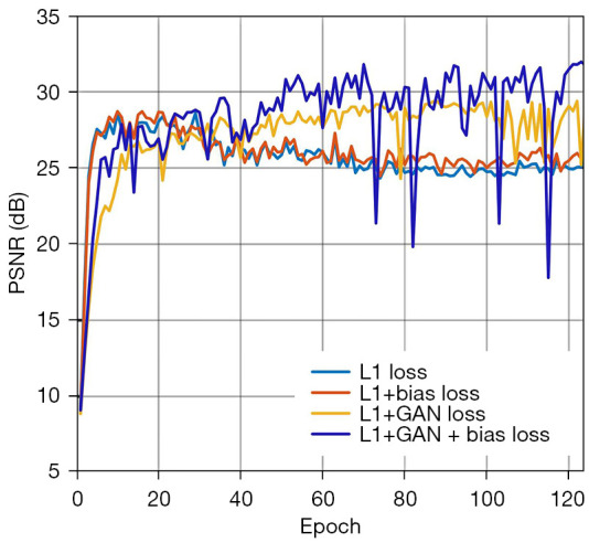
Comparison of the validation process using different loss functions, PSNR vs. training epoch. The larger the PSNR value, the better denoising effect one method can achieve. Proposed combined loss is “L1+GAN+bias loss”. PSNR, peak signal-to-noise ratio; GAN, generative adversarial network.

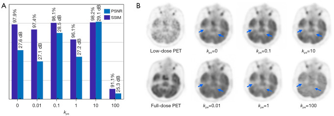
The selection of bias loss weight (λ_p:λ_s) values had a large effect on the trained model. Some values led to a better appearance, while others had no effect or even a negative effect. We focused on studying the effects of different bias loss weights on model bi-c-GAN’s test results. Letting k_ps=λ_p:λ_s, quantitative results and visual examples using different k_ps (0, 0.01, 0.1, 1, 10, and 100) can be seen in Figure 6A and 6B, in which k_ps acts as a baseline for comparisons. In Figure 6A, we found that when k_ps equals 0.1 and 10, the model achieved a better appearance with higher PSNR and SSIM values. Negative transfer occurred when k_ps was very large. As extreme examples, in Figure 6B, the synthesized result of k_ps =10 had more details and a higher black and white contrast, and the visual image of k_ps =100 was the lowest quality.

Figure 6.

The effects of different bias loss weights on synthesized results. (A) The quantitative comparisons of PSNR and SSIM when using different bias loss weighs (k_ps), the chosen kps values here are 0, 0.01, 0.1, 1, 10 and 100. (B) Visual examples of one slice’s synthesized results when using these different bias loss weighs. The first column contains input (5% low-dose PET image) and label (full-dose PET image), and other columns are synthesized images in which the first row appears better than the second row. In two regions of interest which are marked in blue arrows, bad results indicate a lack of details. PSNR, peak signal-to-noise ratio; SSIM, structural similarity; PET, positron emission tomography.

The contribution of conditional inputs

There were four kinds of conditional inputs when training: single-task-based model (like U-net and c-GAN) using low-dose PET modality as the conditional input, single-task-based model using MRI modality as the conditional input, a bi-task-based structure using low-dose PET modality as the primary task’s conditional input and MRI modality as the secondary task’s conditional input, and a bi-task-based structure using MRI modality as the primary task’s conditional input and low-dose PET modality as the secondary task’s conditional input. Using different modalities as conditional inputs when training affected the quality of results.

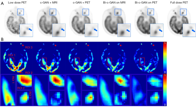
Figure 7 shows visual examples and error maps of one axial slice’s tested results using four selected models. These selected models represent the above-mentioned four kinds of conditional input in which c-GAN was used to represent a single task’s case. First, as shown in Figure 7A, in which both use the c-GAN based model, the one using the MRI modal as a conditional input generated fewer details than the one using PET as the conditional input, but neither generated more details than bi-c-GAN-based methods. Further, using MRI as c-GAN’s conditional input or the primary task’s conditional input of bi-c-GAN influenced the generated results. For example, in the ROI shown on the right downside of each image, there should be two sets of black areas, but MRI-based methods can only clearly generate one set of black areas with the incorrect size and position. A more overall view of the difference between the synthesized images and the ground truth can be shown in Figure 7B, the error maps, and three selected ROI. Again, using PET as conditional input of bi-c-GAN presented fewer differences from the original full-dose PET image than all others with no red area and more blue areas. From ROIs, we again found that methods with MRI as conditional inputs presented a distorted synthesis. Therefore, it was necessary to treat PET as the primary task’s conditional input when training the bi-c-GAN.

Figure 7.

The effects of different conditional inputs on synthesized results. (A) Visual examples and their ROIs of one axial slice’s generating results using different kinds of conditional inputs, the first image is 5% low dose PET image act as original state of PET here, the last image is full dose PET image act as ground truth here, other images here are synthesized results using different models, from left to right: c-GAN conditioned on MRI (c-GAN+MRI); c-GAN conditioned on PET (c-GAN+PET); bi-c-GAN with primary task conditioned on MRI (bi-c-GAN on MRI); bi-c-GAN with primary task conditioned on PET (bi-c-GAN on PET); a ROI is selected from the right upside of the image, which contains two sets of black matters. (B) Error maps of corresponding images in (A). The differences have been normalized to (0, 1), as depicted by the color bars in the right side of error map; blue means a small difference, and red means a large difference. ROI 1 is a large region in the middle of image which marked by red boxes; ROI 2 and 3 are small regions in images’ top and bottle which are marked by red arrows. PERT, positron emission tomography; ROI, region of interest; c-GAN, conditional-generative adversarial network; Bi-c-GAN, bi-task c-GAN; PET, positron emission tomography; MRI, magnetic resonance imaging.

Results

The statistical results from four-fold cross-validation using U-net, c-GAN, M-c-GAN, and the proposed bi-c-GAN are presented here. The PSNR, NMSE, SSIM, and CNR were used as quantitative matrixes to evaluate their effects on improving the quality of 5% low-dose PET images. Another hold-out validation was used to test the effects of the proposed method on other low-dose PETs of 2.5% and 10%. In the comparative results, the superiority of the proposed method over traditional methods was highlighted mainly in three aspects: it had better quantitative achievements, it was better in improving some specific slices, and it was more efficient in improving a wider range of other lose-dose PET of 2.5% and 10%.

Cross-validation

During four-fold cross-validation, 64 datasets were separated into four folds. For each time, three folds were treated as a training set and another one as a test set. The process was repeated four times to yield an overall statistical result. Figure 8 and Table 2 present the detailed comparing results from which we found that the proposed method achieved the best mean (± standard deviation) values and median (Q1/Q3) values in all selected quantitative metrics. The Wilcoxon signed-rank test was used to compare all image quality metrics (95% confidence interval). For example, PSNR was improved by bi-c-GAN from low-dose PET’s 17.36±2.85 dB to 27.2±2.12 dB significantly (P<0.001), compared with U-net 25.98±2.17 dB (P=0.101), c-GAN 26.19±2.41 dB (P=0.025) and M-c-GAN 26.21±2.42 dB (P=0.145). Considering each slice’s initial state is different, we proposed improvement ratios to make comparisons easy, namely, the improvement ratio of PSNR (PIR), NMSE (NIR), SSIM (SIR), and CNR (CIR). These ratios are defined in Eq. [11]:

Figure 8.

Bar plots of quality metrics’ mean and stand deviation values. Four selected evaluating indexes are PSNR, NMSE, SSIM, and CNR. The compared models are U-net, c-GAN, M-c-GAN, and the proposed bi-c-GAN. The 5% low dose PET is also used as a reference to compare in the beginning of each image. PSNR, peak signal-to-noise ratio; NMSE, normalized square error of the mean; SSIM, structural similarity; CNR, contrast noise ratio; PET, positron emission tomography; c-GAN, conditional generative adversarial network; M-c-GAN, multiple c-GAN; Bi-c-GAN, bi-task c-GAN.

Table 2. Comparison of image quality metrics for U-net, c-GAN, M-c-GAN, and the proposed method.

	U-net	c-GAN	M-c-GAN	Proposed
PSNR (dB)
Median (Q1/Q3)	26.4 (24.8/27.5)	26.5 (24.9/28.0)	26.6 (24.6/28.1)	27.5 (26.1/28.6)
PIR (mean ± SD)	11.51%±5.82%	11.69%±5.12%	11.65%±5.10%	13.17±5.84%
P value	0.101	0.025	0.145	<0.001
NMSE (%)
Median (Q1/Q3)	0.309 (0.242/0.445)	0.301 (0.209/0.443)	0.299 (0.210/0.463)	0.242 (0.186/0.340)
NIR (mean ± SD)	70.31%±91.26%	73.55%±86.84%	74.82%±76.02%	81.66%±46.35%
P value	<0.001	<0.001	<0.001	0.016
SSIM
Median (Q1/Q3)	0.981 (0.974/0.986)	0.981 (0.973/0.987)	0.982 (0.974/0.986)	0.985 (0.980/0.987)
SIR (mean ± SD)	26.05%±20.46%	26.02%±19.84%	26.02±19.81%	26.72%±20.69%
P value	<0.001	<0.001	<0.001	0.079
CNR (%)
Median (Q1/Q3)	5.69 (2.64/10.9)	5.79 (2.75/11.0)	6.15 (2.61/11.1)	3.88 (1.72/7.66)
CIR (mean ± SD)	71.76%±49.81%	72.41%±50.34%	72.62%±46.70%	80.60%±32.90%
P value	0.277	0.177	0.526	0.214

P value, Wilcoxon signed-rank test in which significance level was set to be 5% and proposed bi-c-GAN was compared with U-net, c-GAN, M-c-GAN and low-dose PET. Q1/Q3, 25% and 75% percentile values of quartile. PSNR, peak signal to noise ratio; NMSE, normalized mean square error; SSIM, structural similarity; CNR, contrast noise ratio; c-GAN, conditional generative adversarial network; M-c-GAN, multiple c-GAN; PIR, improvement ratio of PSNR; SIR, improvement ratio of SSIM.

$$r_i={\left(-1\right)}^{i-1}\frac{\left|M_i-L{P}_i\right|}{L{P}_i}\cdot 100\%$$ [11]

in which M represents model’s synthesized result, LP represents low-dose PET, i ranging from 1 to 4 is the index of four components in the metric set (1: PSNR, 2: NMSE, 3: SSIM, 4: CNR). By calculating the improvement ratio of each above, results were presented in Table 2, which shows that the average PIR of proposed bi-c-GAN was improved by 6.7–7.3% compared with the other three methods. NIR also improved by 1.3–1.8%, SIR improved by 0.6–0.7%, and CIR improved by 8–8.9%.

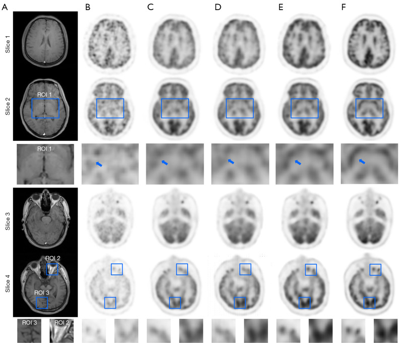
Figure 9 illustrates visual examples of different methods’ effects in four selected slices (selected from up to low regions of the head axial). Both U-net and c-GAN were used to compare the proposed bi-c-GAN. Blue squares indicate three ROIs, and the detail is at the bottom of each image. Visual examples showed that the bi-c-GAN-based model presented more detail than the other two methods, especially in three ROIs. For example, in ROI 2 of slice (4), the proposed bi-c-GAN model synthesized the clearest black matter sets and the compared methods showed a lack of details. Table 3 shows that PIR and SIR were selected to study the bi-c-GAN’s effect on four selected slices over U-net and c-GAN based on the cross-validation experiment; the overall improvement ratio of each was also presented to act as a reference. From Table 3, besides showing the advantage of the proposed bi-c-GAN, we also noticed that the effect of the proposed bi-c-GAN on the upper parts of the head (slice 1 plus slice 2) was more obvious than the effect on the lower parts of the head (slice 3 plus slice 4). The bi-c-GAN’s average PIR in the upper parts was 12.9–17.4% higher than that of U-net and c-GAN compared with its improvement in lower parts (9.2–16.1%). The bi-c-GAN’s average SIR also achieved an improvement of 1.1–1.9% in the upper parts over U-net and c-GAN compared with the lower parts’ improvement of 0.9–1.1%. All these indicated that bi-c-GAN’s effect on improving low-dose PET image quality was more obvious in the upper areas of the head.

Figure 9.

Visual examples of the synthesized PET images by using different methods. Column (A) is T1-weighted MRI; column (B) is 5% low-dose PET images; columns (C), (D) and (E) are synthesized results from U-net, c-GAN, and the proposed method; the last column (F) is the full-dose PET image. Slice 1 to slice 4 are four selected axial parts of the head as shown in Figure 4. Three ROI are also listed in the bottom of slice 2 and slice 4. In ROI 1, a blue arrow was also used to mark one set of black matter. ROI, region of interest; MRI, magnetic resonance imaging; PET, positron emission tomography.

Table 3. The statistical comparison of synthesized results from slices involved in Figure 9. PIR and SIR of U-net, c-GAN, and the proposed bi-c-GAN were presented. Overall achievements acted as references.

Models	Slice 1	Slice 2	Slice 3	Slice 4	Overall
U-net
PIR (%)	59.8±19.9	60.0±18.6	46.7±27.0	48.0±32.1	53.5±25.8
SIR (%)	29.8±19.6	25.8±20.2	21.3±17.7	27.4±23.0	26.1±20.5
c-GAN
PIR (%)	58.2 ±14.7	57.1±12.3	50.6±24.8	51.0±30.7	54.1±22.3
SIR (%)	29.5±18.7	25.3±19.2	21.7±17.2	27.7±22.7	26.0±19.9
Bi-c-GAN
PIR (%)	64.9±19.4	67.8±23.8*	53.5±25.7	57.3±30.0	60.8±25.7
SIR (%)	30.2±20.0*	26.5±21.2	21.9±17.6	28.3±22.8	26.7±20.7

Values are presented in the format of mean ± stand deviation. *, the highest improvement ratio. c-GAN, conditional generative adversarial network; Bi-c-GAN, bi-task c-GAN.

Hold-out validation result

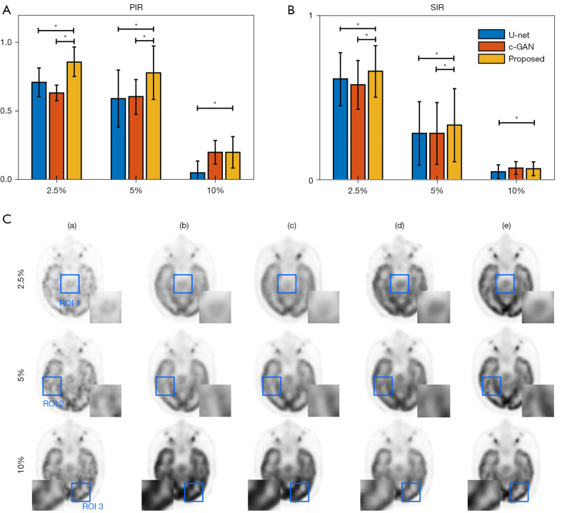
In the hold-out validation, all 64 datasets were used for training, and another 3 datasets were used for testing. During the hold-out validation, the wider effect of our proposed method compared to the other two methods was analyzed. The trained models (trained with 5% low-dose PET as conditional input of bi-c-GAN’s primary task) were tested not only in 5% low-dose PET images but also in 2.5% and 10% low-dose PET images. The statistical results of different methods’ PIR and SIR (mean and standard deviation) values and one slice’s visual examples are presented in Figure 10. The result showed that the bi-c-GAN-based model trained to improve 5% of low-dose PET images’ quality could maintain its advantage and achieved a stable performance in improving 2.5% and 10% of low-dose PET images. At the same time, the performances of other methods tended to vary. For example, Figure 10A shows that the bi-c-GAN presented good preferences for PIR, with an 85.78%±15.22% improvement in the 2.5% low-dose PET compared with U-net’s 81.32%±12.02% (P=0.027) and c-GAN’s 74.72%±6.73% (P=0.019). The bi-c-GAN showed an average improvement ratio of 4.46–6.60%, with a 69.89%±24.31% improvement in the 5% low-dose PET compared with U-net’s 59.22%±25.82% (P=0.003) and c-GAN’s 60.70%±16.70% (P=0.004), and an average improvement ratio of 9.19–10.67%. The bi-c-GAN also showed a 20.03%±11.43% improvement in 10% low-dose PET compared with U-net’s 5.15%±8.56% (P=0.031) and c-GAN’s 20.01%±8.59% (no significance) with an average improvement ratio of 0.01–14.88%. The advantage is also shown in Figure 10C; when compared with the proposed method (column d’s images), synthesized results and their corresponding selected ROIs of U-net (column b’s images) and c-GAN (column c’s images) presented a lack of details in improving 2.5% and 5% low-dose PET images or overfitting in improving 10% low-dose PET images.

Figure 10.

Hold-out validation’s statistical results and visual examples. (A) and (B) are statistical results (mean ± standard deviation) from comparisons using U-net, c-GAN, and the proposed method to improve different initial low-dose PET images of 2.5%, 5%, and 10%: (A) PIR; (B) SIR. The proposed method is compared with two other methods. * indicates a significant result (P<0.05). (C) A visual example is a visual example of different methods’ synthesized results using different levels’ low dose PET inputs: (a) low-dose PET inputs of 2.5%, 5% and 10%; (b) U-net; (c) c-GAN; (d) proposed method; (e) full-dose PET. Three regions of interests are marked by blue boxes. PIR, improvement ratio of peak signal-to-noise ratio; SIR, improvement ratio of structural similarity; PET, positron emission tomography; c-GAN, conditional generative adversarial network.

Discussion

In this paper, bi-task-based bi-c-GAN was trained successfully, demonstrating a high denoising and image quality improving ability. As explained in Methods section, bi-c-GAN is a novel end-to-end encoder-decoder network structure combining the strength of skip connection, conditional input, GAN, and bi-task structure; to make all parts cooperate well, a novel combined loss was used in the training stage. In the ablation experiment, we found that the combined loss contributed to bi-c-GAN’s training by alleviating overfitting and improving training speed though it also could bring instability. Moreover, if the wrong bias loss’s weight was chosen when training using combined loss, a negative transfer occurred. To avoid this, the bias loss’s weight should not be too large, resulting in negative transferring or too small, which will have little effect. Further, conditional input acted differently when contributing to the training result. Although using T1-weighed MRI can provide an inductive bias that benefits the training process, it is not useful when training using MRI as conditional input or as primary task’s conditional input directly because it tends to achieve comparatively lower PSNR and SSIM values, higher NMSE, and CNR values as shown in Table 1. It also has a poor image detail in visual examples, as shown in Figure 7. A potential explanation for this is that although T1-weighted MRI images provide extra information, it is still very different from PET images’ shape and pattern. These differences may remain in the synthesized PET images and then cause distortions in the synthesized PET images.

In the statistical analysis, a four-fold cross-validation was first carried out and tested in 5% low-dose PETs. The bi-c-GAN-based model outperformed U-net, c-GAN, and M-c-GAN-based models with significant results. In the evaluation shown in Figure 8 and Table 2, bi-c-GAN’s has a better denoising ability, which was concluded by higher PSNR values and lower CNR values. These values were more similar to full-dose PET, as indicated by a higher SSIM values and lower NMSE values. Visual examples also showed that bi-c-GAN had more detailed and less distorted results. Moreover, when improving upper slices of the head axial, bi-c-GAN showed more potential, with a higher improvement ratio than the compared methods. This indicates bi-c-GAN’s ability to improve the quality of PET images for these regions. In the hold-out validation, the proposed bi-c-GAN and two comparing models were tested on PET images of various low doses. The statistical results indicated that bi-c-GAN could extend its advantage and effect to improve the quality of 2.5% and 10% of low-dose PET images, demonstrating its more general effect. This can be very useful in a practical situation since a reduced dose will not be an exact amount.

Improving ultra-low-dose PET image quality with deep learning-based methods can be timesaving and financially affordable. Our proposed bi-c-GAN has narrowed the gap in realizing this potential. However, some limitations of bi-c-GAN still exist. First, the bi-task-based structure is very large, and training requires extra resources. Further, the performance of synthesized results is influenced by the combined loss’s weights. Finally, the efficiency of bi-c-GAN needs to be tested in other body parts or a whole-body.

Conclusions

This paper trialed a novel method called bi-c-GAN to improve the quality of ultra-low-dose PET images and reduce patients’ radiation exposure burden. The experimental results from 67 real patients demonstrated the advantage of the proposed method over compared methods in denoising effects, the similarity to full-dose PET, more detail and less distortion in synthesized images, and wider effects. Future work will focus on optimizing our structure and attempting to apply it in a whole-body scenario.

Supplementary

The article’s supplementary files as

Ethical Statement: The authors are accountable for all aspects of the work in ensuring that questions related to the accuracy or integrity of any part of the work are appropriately investigated and resolved. Our study was conducted in accordance with the Declaration of Helsinki (as revised in 2013). Ethical approval (Sun Yat-sen University Cancer Center Guangzhou, China) was obtained, and the informed consent requirement was waived for this retrospective analysis.

References

- 1.Catana C. The Dawn of a New Era in Low-Dose PET Imaging. Radiology 2019;290:657-8. 10.1148/radiol.2018182573 [DOI] [PubMed] [Google Scholar]
- 2.Cherry SR, Jones T, Karp JS, Qi J, Moses WW, Badawi RD. Total-Body PET: Maximizing Sensitivity to Create New Opportunities for Clinical Research and Patient Care. J Nucl Med 2018;59:3-12. 10.2967/jnumed.116.184028 [DOI] [PMC free article] [PubMed] [Google Scholar]
- 3.Karakatsanis NA, Fokou E, Tsoumpas C. Dosage optimization in positron emission tomography: state-of-the-art methods and future prospects. Am J Nucl Med Mol Imaging 2015;5:527-47. [PMC free article] [PubMed] [Google Scholar]
- 4.Hu Z, Xue H, Zhang Q, Gao J, Zhang N, Zou S, Teng Y, Liu X, Yang Y, Liang D, Zhu X, Zheng H. DPIR-Net: Direct PET image reconstruction based on the Wasserstein generative adversarial network. IEEE Trans Radiat Plasma Med Sci 2020;5:35-43. 10.1109/TRPMS.2020.2995717 [DOI] [Google Scholar]
- 5.Zeng T, Gao J, Gao D, Kuang Z, Sang Z, Wang X, Hu L, Chen Q, Chu X, Liang D, Liu X, Yang Y, Zheng H, Hu Z. A GPU-accelerated fully 3D OSEM image reconstruction for a high-resolution small animal PET scanner using dual-ended readout detectors. Phys Med Biol 2020;65:245007. 10.1088/1361-6560/aba6f9 [DOI] [PubMed] [Google Scholar]
- 6.Zhang W, Gao J, Yang Y, Liang D, Liu X, Zheng H, Hu Z. Image reconstruction for positron emission tomography based on patch-based regularization and dictionary learning. Med Phys 2019;46:5014-26. 10.1002/mp.13804 [DOI] [PMC free article] [PubMed] [Google Scholar]
- 7.Hu Z, Li Y, Zou S, Xue H, Sang Z, Liu X, Yang Y, Zhu X, Liang D, Zheng H. Obtaining PET/CT images from non-attenuation corrected PET images in a single PET system using Wasserstein generative adversarial networks. Phys Med Biol 2020;65:215010. 10.1088/1361-6560/aba5e9 [DOI] [PubMed] [Google Scholar]
- 8.Kang J, Gao Y, Shi F, Lalush DS, Lin W, Shen D. Prediction of standard-dose brain PET image by using MRI and low-dose brain 18FFDG PET images. Med Phys 2015;42:5301-9. 10.1118/1.4928400 [DOI] [PMC free article] [PubMed] [Google Scholar]
- 9.Wang Y, Zhang P, An L, Ma G, Kang J, Shi F, Wu X, Zhou J, Lalush DS, Lin W, Shen D. Predicting standard-dose PET image from low-dose PET and multimodal MR images using mapping-based sparse representation. Phys Med Biol 2016;61:791-812. 10.1088/0031-9155/61/2/791 [DOI] [PubMed] [Google Scholar]
- 10.Zhang Q, Gao J, Ge Y, Zhang N, Yang Y, Liu X, Zheng H, Liang D, Hu Z. PET image reconstruction using a cascading back-projection neural network. IEEE J Sel Top Signal Process 2020;14:1100-11. 10.1109/JSTSP.2020.2998607 [DOI] [Google Scholar]
- 11.Qi J. Theoretical evaluation of the detectability of random lesions in Bayesian emission reconstruction. Inf Process Med Imaging 2003;18:354-65. 10.1007/978-3-540-45087-0_30 [DOI] [PubMed] [Google Scholar]
- 12.Wangerin KA, Ahn S, Wollenweber S, Ross SG, Kinahan PE, Manjeshwar RM. Evaluation of lesion detectability in positron emission tomography when using a convergent penalized likelihood image reconstruction method. J Med Imaging (Bellingham) 2017;4:011002. 10.1117/1.JMI.4.1.011002 [DOI] [PMC free article] [PubMed] [Google Scholar]
- 13.Wang T, Lei Y, Fu Y, Curran WJ, Liu T, Nye JA, Yang X. Machine learning in quantitative PET: A review of attenuation correction and low-count image reconstruction methods. Phys Med 2020;76:294-306. 10.1016/j.ejmp.2020.07.028 [DOI] [PMC free article] [PubMed] [Google Scholar]
- 14.Häggström I, Schmidtlein CR, Campanella G, Fuchs TJ. DeepPET: A deep encoder-decoder network for directly solving the PET image reconstruction inverse problem. Med Image Anal 2019;54:253-62. 10.1016/j.media.2019.03.013 [DOI] [PMC free article] [PubMed] [Google Scholar]
- 15.Olveres J, González G, Torres F, Moreno-Tagle JC, Carbajal-Degante E, Valencia-Rodríguez A, Méndez-Sánchez N, Escalante-Ramírez B. What is new in computer vision and artificial intelligence in medical image analysis applications. Quant Imaging Med Surg 2021;11:3830-53. 10.21037/qims-20-1151 [DOI] [PMC free article] [PubMed] [Google Scholar]
- 16.Greco F, Mallio CA. Artificial intelligence and abdominal adipose tissue analysis: a literature review. Quant Imaging Med Surg 2021;11:4461-74. 10.21037/qims-21-370 [DOI] [PMC free article] [PubMed] [Google Scholar]
- 17.Caruana R. Multitask learning. Mach Learn 1997;28:41-75. 10.1023/A:1007379606734 [DOI] [Google Scholar]
- 18.Ruder S. An overview of multi-task learning in deep neural networks. arXiv preprint arXiv:05098 2017.
- 19.Krizhevsky A, Sutskever I, Hinton GE. ImageNet classification with deep convolutional neural networks. In: Pereira F, Burges CJ, Bottou L, Weinberger KQ. Editors. Advances in Neural Information Processing Systems 25 (NIPS 2012). 2012;25:1097-105. [Google Scholar]
- 20.Gong K, Guan J, Liu CC, Qi J. PET Image Denoising Using a Deep Neural Network Through Fine Tuning. IEEE Trans Radiat Plasma Med Sci 2019;3:153-61. 10.1109/TRPMS.2018.2877644 [DOI] [PMC free article] [PubMed] [Google Scholar]
- 21.Wang YJ, Baratto L, Hawk KE, Theruvath AJ, Pribnow A, Thakor AS, Gatidis S, Lu R, Gummidipundi SE, Garcia-Diaz J, Rubin D, Daldrup-Link HE. Artificial intelligence enables whole-body positron emission tomography scans with minimal radiation exposure. Eur J Nucl Med Mol Imaging 2021;48:2771-81. 10.1007/s00259-021-05197-3 [DOI] [PMC free article] [PubMed] [Google Scholar]
- 22.Zhu B, Liu JZ, Cauley SF, Rosen BR, Rosen MS. Image reconstruction by domain-transform manifold learning. Nature 2018;555:487-92. 10.1038/nature25988 [DOI] [PubMed] [Google Scholar]
- 23.Chen KT, Toueg TN, Koran MEI, Davidzon G, Zeineh M, Holley D, Gandhi H, Halbert K, Boumis A, Kennedy G, Mormino E, Khalighi M, Zaharchuk G. True ultra-low-dose amyloid PET/MRI enhanced with deep learning for clinical interpretation. Eur J Nucl Med Mol Imaging 2021;48:2416-25. 10.1007/s00259-020-05151-9 [DOI] [PMC free article] [PubMed] [Google Scholar]
- 24.Ronneberger O, Fischer P, Brox T. editors. U-net: Convolutional networks for biomedical image segmentation. International Conference on Medical image computing and computer-assisted intervention; Springer; 2015. [Google Scholar]
- 25.Pathak D, Krahenbuhl P, Donahue J, Darrell T, Efros AA. editors. Context encoders: Feature learning by inpainting. Proceedings of the IEEE conference on computer vision and pattern recognition; 2016. [Google Scholar]
- 26.Goodfellow I, Pouget-Abadie J, Mirza M, Xu B, Warde-Farley D, Ozair S, Courville A, Bengio Y. editors. Generative adversarial nets. Advances in neural information processing systems; 2014. [Google Scholar]
- 27.Wang Y, Zhou L, Yu B, Wang L, Zu C, Lalush DS, Lin W, Wu X, Zhou J, Shen D. 3D Auto-Context-Based Locality Adaptive Multi-Modality GANs for PET Synthesis. IEEE Trans Med Imaging 2019;38:1328-39. 10.1109/TMI.2018.2884053 [DOI] [PMC free article] [PubMed] [Google Scholar]
- 28.Isola P, Zhu JY, Zhou T, Efros AA. Image-to-image translation with conditional adversarial networks. 2017 IEEE Conference on Computer Vision and Pattern Recognition (CVPR), 2017:5967-76. [Google Scholar]
- 29.Wang Y, Yu B, Wang L, Zu C, Lalush DS, Lin W, Wu X, Zhou J, Shen D, Zhou L. 3D conditional generative adversarial networks for high-quality PET image estimation at low dose. Neuroimage 2018;174:550-62. 10.1016/j.neuroimage.2018.03.045 [DOI] [PMC free article] [PubMed] [Google Scholar]
- 30.Mirza M, Osindero S. Conditional generative adversarial nets. arXiv preprint arXiv:05098 2014.
- 31.Wang TC, Liu MY, Zhu JY, Tao A, Kautz J, Catanzaro B. High-resolution image synthesis and semantic manipulation with conditional gans. 2018 IEEE/CVF Conference on Computer Vision and Pattern Recognition, 2018:8798-807. [Google Scholar]
- 32.Cui J, Gong K, Guo N, Wu C, Meng X, Kim K, Zheng K, Wu Z, Fu L, Xu B, Zhu Z, Tian J, Liu H, Li Q. PET image denoising using unsupervised deep learning. Eur J Nucl Med Mol Imaging 2019;46:2780-9. 10.1007/s00259-019-04468-4 [DOI] [PMC free article] [PubMed] [Google Scholar]
- 33.Onishi Y, Hashimoto F, Ote K, Ohba H, Ota R, Yoshikawa E, Ouchi Y. Anatomical-guided attention enhances unsupervised PET image denoising performance. Med Image Anal 2021;74:102226. 10.1016/j.media.2021.102226 [DOI] [PubMed] [Google Scholar]
- 34.Chen KT, Gong E, de Carvalho Macruz FB, Xu J, Boumis A, Khalighi M, Poston KL, Sha SJ, Greicius MD, Mormino E, Pauly JM, Srinivas S, Zaharchuk G. Ultra-Low-Dose 18F-Florbetaben Amyloid PET Imaging Using Deep Learning with Multi-Contrast MRI Inputs. Radiology 2019;290:649-56. 10.1148/radiol.2018180940 [DOI] [PMC free article] [PubMed] [Google Scholar]
- 35.Pan SJ, Yang Q. A survey on transfer learning. IEEE Trans Knowl Data Eng 2009;22:1345-59. 10.1109/TKDE.2009.191 [DOI] [Google Scholar]
- 36.Patel VM, Gopalan R, Li R, Chellappa R. Visual domain adaptation: A survey of recent advances. IEEE Signal Process Mag 2015;32:53-69. 10.1109/MSP.2014.2347059 [DOI] [Google Scholar]
- 37.Hajiramezanali E, Dadaneh SZ, Karbalayghareh A, Zhou M, Qian X. Bayesian multi-domain learning for cancer subtype discovery from next-generation sequencing count data. Advances in Neural Information Processing Systems; 2018. [Google Scholar]
- 38.Kuga R, Kanezaki A, Samejima M, Sugano Y, Matsushita Y. Multi-task learning using multi-modal encoder-decoder networks with shared skip connections. Proceedings of the IEEE International Conference on Computer Vision Workshops; 2017. [Google Scholar]
- 39.Eitel A, Springenberg JT, Spinello L, Riedmiller M, Burgard W. Multimodal deep learning for robust RGB-D object recognition. 2015 IEEE/RSJ International Conference on Intelligent Robots and Systems (IROS), 2015: 681-7. [Google Scholar]
Associated Data
This section collects any data citations, data availability statements, or supplementary materials included in this article.
Supplementary Materials