Dual-polarity voltage imaging of the concurrent dynamics of multiple neuron-types

Abstract

Genetically encoded fluorescent voltage indicators are ideally suited to reveal the millisecond-scale interactions among and between targeted cell populations. However, current indicators lack the requisite sensitivity for in vivo multipopulation imaging. We describe next-generation green and red voltage-sensors, Ace-mNeon2 and VARNAM2, and their reverse response-polarity variants pAce and pAceR. Our indicators enable 0.4–1 kHz voltage recordings from >50 spiking neurons per field-of-view in awake mice and ~30-min continuous imaging in flies. Using dual-polarity multiplexed imaging, we uncovered brain state-dependent antagonism between neocortical SST⁺ and VIP⁺ interneurons and contributions to hippocampal field potentials from cell ensembles with distinct axonal projections. By combining three mutually compatible indicators, we performed simultaneous triple-population imaging. These approaches will empower investigations of the dynamic interplay between neuronal subclasses at single-spike resolution.

One Sentence Summary:

A new suite of voltage sensors enables simultaneous activity imaging at cellular resolution from multiple neuronal classes in awake animals.

The dynamic interplay of multiple excitatory and inhibitory neuronal subclasses is central to how the brain processes information. During motor or sensory processing, the external environment and an animal’s internal state can impact the activity of neocortical interneurons, which in turn modulate excitatory projection neurons (1–5). Likewise, in hippocampus, different ensembles of projection neurons exhibit state-dependent changes in spiking activity related to learning and memory (6–9). However, how different neural subclasses coordinate their dynamics in real-time remains poorly understood, due to an inability to measure the spiking activity of two or more genetically defined or projection-targeted neural ensembles simultaneously.

Genetically encoded voltage indicators (GEVIs) enable targeted recordings of spiking and subthreshold activity with sub-millisecond temporal precision (10–12). Although extensive protein engineering has spawned a host of new sensors (13–24), existing GEVIs are not optimized for concurrent, targeted recordings from two or more cell classes in behaving animals.

We previously introduced the green and red fluorescence resonance energy transfer (FRET)-opsin GEVIs, Ace-mNeon and VARNAM (17, 18). FRET-opsin GEVIs are fusions of a bright fluorescent protein (FP, the FRET donor) to a transmembrane opsin with a voltage-sensitive light absorption spectrum (the FRET acceptor) (25, 26). This modular design enables voltage-imaging in live animals with a high dynamic range of fluorescence signaling but at far lower illumination levels (~25 mW mm⁻²) than those (1–10 W mm⁻²) required by opsin voltage indicators (16, 19, 22, 23, 27). Imaging studies using FRET-opsins have generally monitored the time-dependent emissions of the bright FRET donor but not those of the opsin FRET acceptor, since the latter’s fluorescence is too dim to augment the detection of voltage signals. Thus, only one fluorescence channel is needed to image a FRET-opsin GEVI, with excitation and emission wavelength bandwidths matching those of the bright donor (17, 18, 25). Ace-mNeon and VARNAM both comprise fusions of the Acetabularia (Ace) rhodopsin (17, 18) to bright FPs, mNeonGreen (28) and mRuby3 (29), respectively. Notably, Ace-mNeon and VARNAM have demonstrated optical compatibility for concurrent recordings in live flies (18).

Protein engineering of negative and positive polarity FRET-opsins

To improve the sensitivities of Ace-mNeon and VARNAM for recordings in awake mice, we performed protein engineering and high-throughput screening of voltage responsivity in excitable human embryonic kidney (HEK) cells (Fig. 1, A and B) (18, 30, 31). Our screening platform scores GEVIs for brightness, voltage sensitivity, and kinetics in a plate-based format, achieving a capacity of 120 unique variants/day with a sample content of ~2000 cells/variant (18).

Fig. 1. Design and characterization of Ace-mNeon2, VARNAM2 and reverse polarity variants pAce and pAceR.

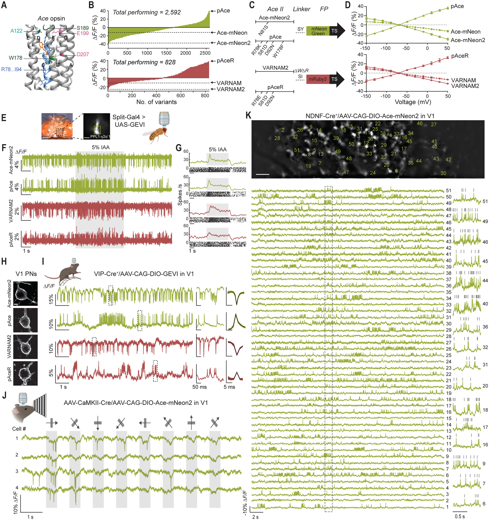
(A) Crystal structure of Ace (PDB ID: 3AM6), showing residues targeted for site-directed saturation mutagenesis on Ace-mNeon and VARNAM. The 7 transmembrane helices are labeled A through G. AAs R78 through I94 on helix C and specified loci on other helices were targeted.

(B) Distribution of fluorescence responses to field stimulation acquired from spiking HEK cells expressing Ace-mNeon (top) and VARNAM (bottom) variants obtained on the high-throughput platform.

(C) Schematic representations of Ace-mNeon2, pAce, VARNAM2, and pAceR constructs, depicting the point mutations in Ace and the Ace-FP linker.

(D) ΔF/ΔV curves obtained using whole-cell recordings and concurrent fluorescence imaging of HEK cells transfected with Ace-mNeon, Ace-mNeon2, and pAce (top), and VARNAM, VARNAM2, and pAceR (bottom). Values represent mean ± S.E.M.

(E) In vivo voltage imaging through a transparent surgical window implanted on a fly head (left). Each of the indicators was selectively expressed in PPL1-γ2α’1 dopaminergic neuron using a split-GAL4 system (right). Yellow dashed box indicates the axonal region of PPL1-γ2α’1.

(F) Representative recordings from PPL1-γ2α’1 using the four GEVIs, showing odor-evoked spiking elicited by 5 s delivery (gray shading) of 5% isoamyl acetate.

(G) Top panels: Mean ± S.E.M. spiking rates during odor delivery and raster plots of individual trials (n = 10 trials, 2 trials/fly).

(H) Confocal images from coronal cortical slices of V1 PNs expressing the indicated sensors. Scale bar: 5 μm.

(I) Left, example fluorescence traces showing spontaneous spiking obtained from awake, head-restrained mice selectively expressing the indicators in V1 VIP⁺ interneurons; Center, the boxed areas on the traces are shown at an expanded timescale; Right, Mean ± S.E.M. optical spike waveform (n=5 neurons per condition ranked in order of decreasing signal-to-noise ratios, 3 mice each (Ace-mNeon2 and pAce) and 2 mice each (VARNAM2 and pAceR)).

(J) Example visual responses from layer 2/3 PNs to drifting gratings presented at 8 different orientations, acquired using Ace-mNeon2 in an awake mouse. Arrows indicate stimulus orientation. Gray shading denotes stimulus periods.

(K) Top, Representative epifluorescence image of a single field-of-view from a NDNF-Cre⁺ mouse expressing Cre-dependent soma-targeted Ace-mNeon2 in V1. Scale bar: 50 μm. Bottom, ΔF/F traces showing spontaneous activity from regions-of-interest (ROIs), numbered in the image above. Fluorescence traces are inverted for visualization. Boxed region is shown at an expanded timescale on the right for select cells. Grey ticks denote identified spikes.

In Ace-mNeon and VARNAM, depolarization-dependent quenching by Ace of fluorescence from the FP leads to depolarization-evoked fluorescence decreases as the readout of voltage changes. To improve voltage sensitivity, we sought to enhance the FRET transfer by optimizing the Ace-FP linker (32). In Ace-mNeon, we also performed site-saturation mutagenesis at Ace N81 (Fig. 1A, and fig. S1) (18). Screening of mutagenic libraries uncovered variants with increased response amplitudes (Fig. 1B, and fig. S2). Ace-mNeon N81S G229Y and VARNAM Δ228W Δ229R G231I (henceforth, Ace-mNeon2 and VARNAM2, respectively) exhibited significantly improved fluorescence responses to depolarizing voltages compared to their predecessors in patch-clamp recordings from transfected cells (ΔF/F for 120 mV step were (mean ± S.E.M.): −31.3 ± 0.7% for Ace-mNeon2 (n=13 cells) versus −13.9 ± 0.6% for Ace-mNeon (n=11 cells), P<0.0001, Mann-Whitney test; −22.9 ± 0.7% for VARNAM2 (n=13 cells) versus −14.1 ± 0.5% for VARNAM (n=8 cells), P<0.0001, Mann-Whitney test) (Fig. 1, C, and D, and fig. S3, S4, and S5, and Table S1).

We next screened a library of Ace-mNeon2 D92X positional mutants, owing to the highly conserved role of the N81/D92 pair in opsin proton-pumping and photosensing (33, 34). We uncovered several variants with response polarity reversals that exhibited fluorescence increases during depolarization (fig. S6). Although the best-performing positive variant Ace-mNeon2 D92N exhibited slower kinetics, reciprocal S81X saturation mutagenesis revealed kinetics rescue mutants (fig. S6, and S7). The 92N/81D reversed polarity phenotype is transposable across other Ace-based indicators, including VARNAM and Voltron (13, 18).

For further engineering, we targeted residues lining Ace’s photosensing helix C, amino acids involved in stabilizing its voltage-sensitive intermediate state, and those nearby the chromophore (Fig. 1A, and fig. S1) (34–36). Voltage screening of mutagenic libraries uncovered positive variants with enhanced sensitivities (fig. S8). Ace-mNeon2 R78K S81D D92N W178F and VARNAM2 R78E S81D D92N, henceforth pAce (positive Ace) and pAceR (positive Ace in Red), exhibited ΔF/F values of 36.6 ± 0.7% (mean ± S.E.M.) and 33.4 ± 1.1% (n=11 cells each), respectively, per 120 mV in cultured HEK cells (Fig. 1, B–D, and fig. S5, S9, and S10). As these positive variants have the same signaling dynamic range as Ace-mNeon2 and VARNAM2 but in the opposite direction, they have slightly lower resting fluorescence intensities than the latter and reduced resting-state photobleaching, similar to other positive GEVIs (Fig. S11) (14, 37).

All indicators except pAceR showed sub-millisecond kinetics at room temperature (fig. S5, and Table S1). Overall, Ace-mNeon2, VARNAM2, and pAce exhibited the largest effective ΔF/F (%) for single action potentials (APs) compared to prior negative- and positive-polarity GEVIs in 1-ms impulse response computations (fig. S12, and Table S1).

Sensor characterization in awake flies and mice

For voltage imaging in live animals, we used high-speed (400 or 600 Hz in mice, 1 kHz in fruit flies), widefield one-photon epifluorescence microscopy, for all studies described in this paper.

We first expressed each of our 4 GEVIs in the PPL1-γ2α’1 dopaminergic neuron in flies, in which they reported spontaneous and odor-evoked spiking with comparable baseline- and evoked spike rates (Fig. 1, E–G). Compared to their red counterparts, the green GEVIs exhibited greater response amplitudes and values of d’, a signal detection theory metric characterizing how the ratio of fluorescence signals to background fluctuations sets the spike detection fidelity (38) (ΔF/F, d’ (mean ± S.E.M.): 3.1 ± 0.2%, 14.5 ± 1.4 (Ace-mNeon2); 4.0 ± 0.1%, 13.4 ± 0.8 (pAce); 1.1 ± 0.1%, 7.4 ± 0.4 (VARNAM2); 0.9 ± 0.03%, 6.5 ± 0.3 (pAceR)). We also compared the performance of all 4 GEVIs in the PPL1-α’2α2 neuron, where they had greater d’ values than their parent indicators Ace-mNeon and VARNAM (~10.8 (Ace-mNeon2), ~8.7 (pAce), ~7.0 (VARNAM2) and ~6.7 (pAceR) versus reported values of ~6.9 (Ace-mNeon) and ~6.6 (VARNAM)) (fig. S13) (18). pAce’s higher ΔF/F values and superior photostability enabled extended duration (30-min) continuous recordings with stable d’ values throughout imaging sessions with illumination powers of ~5 mW mm⁻² (fig. S14).

For studies in live mice, our epifluorescence imaging methodology was designed to allow cellular resolution recordings in cortical brain tissue and to reduce both tissue autofluorescence and background fluorescence from scattered or out-of-focus indicator emissions. Specifically, we (i) were able to use modest illumination intensities (typically, 25 mW mm⁻²), owing to the high brightness of our indicators; (ii) achieved relatively sparse fluorescence labeling (<370 labeled cells per mm²) by targeting specific cell classes through virally mediated projection targeting or using cell-type specific, Cre- or Flp-driver mouse lines (39–42); (iii) generated soma-targeted versions of Ace-mNeon2, VARNAM2, pAce and pAceR, which mainly trafficked to cell body membranes (Fig. 1H) (43). With this labeling and trafficking approach, <4.2% (and usually much less) of the area of each imaging plane was occupied by labeled cell bodies. Further, for data analyses, we used cell extraction algorithms designed to determine neuronal activity traces with minimal contamination from physiologic artifacts or background activity (44–46) (fig. S15 and Methods).

We expressed each of our 4 GEVIs in vasoactive intestinal peptide-expressing (VIP⁺) interneurons in primary visual cortex (V1), in which they successfully reported single action potentials (Fig. 1, H and I). The ΔF/F values per spike were (mean ± S.E.M.): −16.5 ± 1.9% for Ace-mNeon2 (n=127 spikes), 10.7 ± 1.4% for pAce (n=87 spikes), −7.3 ± 1.2% for VARNAM2 (n=49 spikes) and 3.2 ± 0.5% for pAceR, (n=48 spikes).

To record stimulus-evoked activity, we used axonal projection targeting to express our best-performing GEVI, Ace-mNeon2, in a sparse subset of V1 layer 2/3 pyramidal neurons (PNs) ~100–200 μm beneath the pia (Fig. 2E). Specifically, we targeted PNs projecting to the anteromedial visual cortical area (AM) (39, 42), by injecting an adeno-associated virus (AAV) expressing Cre-dependent Ace-mNeon2 into area V1 of wild-type mice, plus a retrograde AAV expressing Cre via the CaMKII promoter into AM. Voltage imaging of these V1→AM projecting neurons during presentations of drifting grating visual stimuli revealed the cells’ orientation-selective visual responses (Fig. 1J).

Fig. 2. Ace-mNeon2 voltage imaging unveils state-dependent modulation of spontaneous firing in excitatory and inhibitory cell classes in V1.

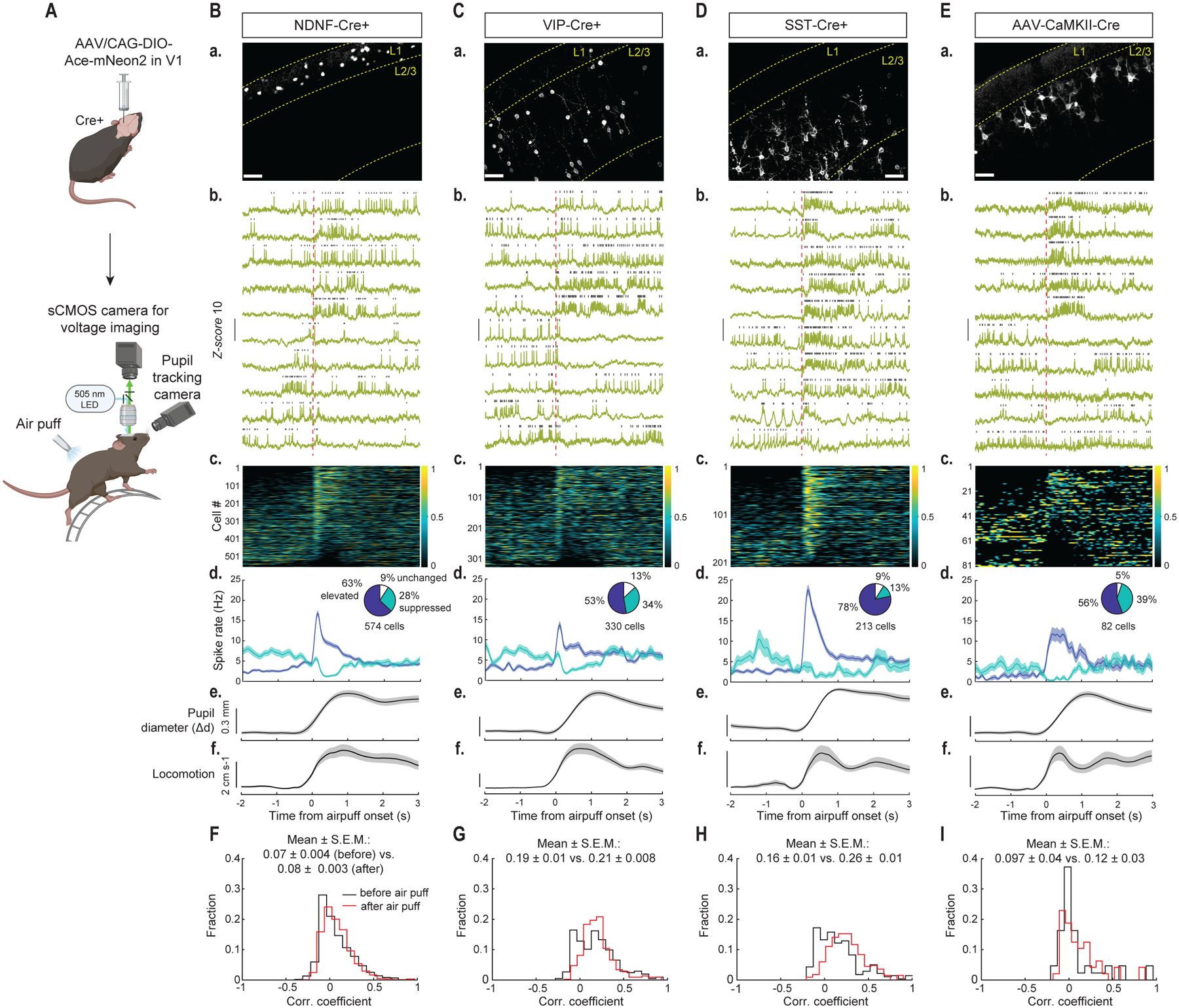
(A) Schematic of AAV injection and experimental setup.

(B) (a) Confocal images of soma-targeted Ace-mNeon2 expression in NDNF⁺ interneurons. Scale bar: 50 μm. (b) Representative fluorescence-time traces from individual cells (inverted for visualization purposes). Vertical dashed line in red indicates air puff onset. Grey ticks denote identified spikes. (c) Z-scored firing rate for all NDNF⁺ interneurons (n=574 cells, 6 mice). Cells are arranged in order of decreasing spike modulation indices (Methods). (d) Mean ± S.E.M. firing rate aligned to air puff onset for activated (dark blue) and suppressed (cyan) fractions. Pie chart insets indicate % of cells with elevated (dark blue), suppressed (cyan) or unchanged (white) spike rates following air puff. (e) Mean ± S.E.M. pupil diameter and (f) locomotor speed.

(C) Same as (B) for VIP⁺ interneurons (n=330 cells, 5 mice).

(D) Same as (B) for SST⁺ interneurons (n=213 cells, 6 mice).

(E) Same as (B) for PNs (n=82 cells, 4 mice).

(F) Distribution of pairwise correlation coefficients of mean firing rates across a sliding 20-ms-window, as determined for 3-s-intervals, before (black) and after (red) air puff for NDNF⁺ interneurons (2300 cell pairs in the same fields-of-view, 6 mice; **P=0.0021; Wilcoxon matched-pairs signed rank test for before vs. after air puff). The mean ± S.E.M. correlation coefficient values are shown above the distribution plots.

(G) Same as (F) for VIP⁺ interneurons (n=442 pairs, 5 mice; **P=0.0011).

(H) Same as (F) for SST⁺ interneurons (n=334 pairs, 6 mice; ***P<0.0001).

(I) Same as (F) for PNs (n=51 pairs, 4 mice; *P=0.03).

To showcase imaging of neural ensemble dynamics, we used Cre-driver mice to target Ace-mNeon2 to neuron-derived neurotrophic factor expressing (NDNF⁺) interneurons, ~50–70 μm below the pia (41, 47, 48) (Fig. 2B), and recorded spiking in up to 51 cells at once (Fig. 1K), for 4–5 min continuously (fig. S16). Similarly, using other Cre- or Flp-driver lines, we respectively targeted Ace-mNeon2 or pAce to layer 2/3 somatostatin-expressing (SST⁺) interneurons (~200–350 μm deep, (40)) or VIP⁺ interneurons (~50–300 μm below the pia, (49)), to capture voltage signals from multiple cells of each cell class (Fig. 2, C and D; fig. S17). Across these different cortical cell-types, d’ values ranged from 9.9–17.5, implying spike detection error rates ranging from 0.04 spike min^–1 to infinitesimal values (fig. S18) (38). This high level of spike detection fidelity allowed us to extract spike trains and spike timing estimates that were invariant to the use of different cell extraction algorithms (fig. S15, A, B, D, and G).

Voltage imaging of visual cortical ensembles during behavioral state transitions

In neocortex, interneuron activity is strongly influenced by an animal’s internal state and, in turn, modulates excitatory cells (1–5). However, the extent to which different interneuron subclasses respond to state transitions and how distinct brain states impact the millisecond-scale interactions between neuron classes remain unknown.

To address these questions, we selectively targeted Ace-mNeon2 to NDNF⁺, VIP⁺ or SST⁺ interneurons in area V1, or to V1→AM projecting neurons, by using the same mouse lines and viruses as above (Fig. 2A) (40, 41). Voltage imaging in V1 of awake, head-restrained mice revealed spontaneous spiking rates (mean ± S.E.M.) of 4.72 ± 0.01 Hz for NDNF⁺ neurons (n=192 cells, 7 mice), 6.52 ± 0.23 Hz for VIP⁺ neurons (n=49 cells, 5 mice), 4.71 ± 0.21 Hz for SST⁺ neurons (n=43 cells, 5 mice), and 0.93 ± 0.34 Hz for PNs (n=53 cells, 5 mice). These values are consistent with estimated spike rates of V1 layer 2/3 PNs and SST⁺ cells obtained via electrophysiological recordings in awake mice (4, 50). Likewise, the higher spontaneous firing rates of VIP⁺ versus SST⁺ interneurons have been observed across distinct cortical areas (51, 52).

To induce a change in brain state by increasing arousal, we delivered a brief air puff to the mouse’s back while monitoring its pupil diameter, which is a commonly used, simple metric of arousal (Fig. 2A) (53, 54). The evoked arousal was often accompanied by the onset of locomotion and robust modulations of spiking across all neuron classes studied (Fig. 2, B–E). However, the distinct cell classes differed regarding both the fractions of cells that increased or decreased their spiking and the magnitudes of spike rate modulation (Fig. 2, B–E).

We imaged the spiking dynamics of ~1200 neurons across the different cell-types. Upon arousal, SST⁺ interneurons exhibited the most substantial state-dependent modulation, with 78% of SST⁺ cells increasing their spontaneous spiking rates and only 13% decreasing their spiking (Fig. 2D). SST⁺ cells also underwent the greatest increases in spike rates among the cell types imaged, from 2.5 ± 0.4 Hz (mean ± S.E.M.) under baseline conditions to 22.5 ± 1.2 Hz after air puff (Fig. 2D). 63% of NDNF⁺ interneurons also increased their spiking, from 2.6 ± 0.3 Hz to 16.8 ± 0.7 Hz, whereas 28% decreased their spiking after air puff (Fig. 2B). VIP⁺ neurons and PNs exhibited comparable state-dependent responses, with half of each population showing elevated (53% and 56%, respectively) and a third showing suppressed spiking after air puff (34% and 39%, respectively). These latter two classes also had similar spike rate increases during arousal (from 3.8 ± 0.5 Hz to 13.7 ± 0.8 Hz for VIP⁺ cells, and 0.9 ± 0.3 Hz to 11.8 ± 1.6 Hz for PNs) (Fig. 2, C and E). That each neuron-type studied exhibited a subset of cells that decreased their spiking argues against the possibility that the net spiking increases were motion-related artifacts stemming from the locomotion that often occurred after the air puff. Further supporting this point, on air puff trials in which there was no locomotor increase, we still observed comparable modulations in neural activity (fig. S19). Among the cell types imaged, the air puff-evoked rise in spiking among SST⁺ cells returned the fastest toward baseline levels, whereas VIP⁺ and NDNF⁺ interneurons, which receive inhibitory inputs from SST⁺ cells (55, 56), returned more gradually to baseline spiking levels (Fig. 2, B–D).

To characterize the degree of spiking synchronization between the cells of each type, we computed pairwise correlation coefficients for the time-dependent spike rates of each cell pair, and compared the distributions of these coefficients as determined, before versus after air puff. Both SST⁺ and VIP⁺ cells exhibited positive intra-population coupling of spontaneous activity (57), which rose slightly during arousal, especially among SST⁺ cells. By comparison, NDNF⁺ interneurons and PNs showed weaker intra-population correlations (58), which were unaltered by air puff (Fig. 2, F–I).

Dual polarity multiplexed voltage imaging

While arousal increases the net spontaneous activity of multiple cell subtypes (Fig. 2), whether the fine-scale dynamic relationships between two or more subtypes are also altered remains unknown. Thus, we turned to simultaneous multipopulation voltage imaging using our improved GEVIs.

Multipopulation recordings using fluorescent Ca²⁺ or voltage sensors were previously done by targeting spectrally orthogonal sensors to distinct cell-types (18, 59–62). We reasoned that a pair of GEVIs operating in the same spectral channel but with opposite response-polarities should be mutually compatible, allowing studies of two cell-types per color channel. The cells of each type can be distinguished by the directionality of their optical spike waveforms (fig. S20).

We performed dual-polarity multiplexed voltage imaging (DUPLEX) in awake mice, where we targeted Ace-mNeon2 and pAce to either two distinct inhibitory or to one excitatory plus one inhibitory cell types, by using Cre and Flp-dependent expression strategies (Fig. 3A and Methods). We virally expressed Cre-dependent Ace-mNeon2 and Flp-dependent pAce in area V1 of NDNF-Cre⁺/VIP-Flp⁺ or SST-Cre⁺/VIP-Flp⁺ double transgenic mice. Alternatively, we injected recombinase-dependent Ace-mNeon2 and pAce viruses plus AAV-CaMKII-Cre into VIP-Flp⁺ mice (fig. S21). High-speed epifluorescence imaging in a single color channel revealed the joint dynamics of NDNF⁺ and VIP⁺ cells, SST⁺ and VIP⁺ cells, or PNs and VIP⁺ cells, respectively, in these mice while they were awake but head-restrained (Fig. 3, B–G, and fig. S21).

Fig. 3. DUPLEX captures the concerted activation dynamics between cell class pairs in V1.

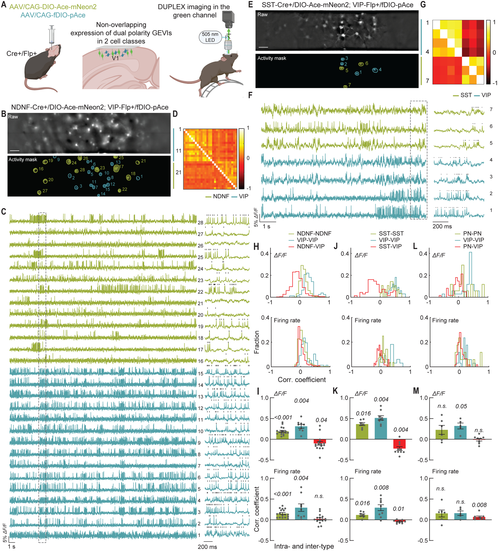
(A) Schematic of AAV injections and experimental setup.

(B-F) Example DUPLEX recordings from two targeted cell classes.

(B-E) Raw epifluorescence (top) and activity-mask (bottom) images of single fields-of-view from a (B) NDNF-Cre⁺/VIP-Flp⁺ mouse expressing Ace-mNeon2 in NDNF⁺ interneurons (green) and pAce in VIP⁺ cells (blue), and (E) SST-Cre⁺/VIP-Flp⁺ mouse expressing Ace-mNeon2 in SST⁺ interneurons (green) and pAce in VIP⁺ interneurons (blue). Active regions-of-interest (ROIs) are numbered. Scale bar: 50 μm.

(C-F) ΔF/F traces from the ROIs numbered in (B) and (E), respectively. Ace-mNeon2 traces are inverted for visualization purposes. The boxed region in (B) is shown at an expanded timescale to the right. Grey ticks indicate identified spikes.

(D-G) Intra- and inter-population correlation coefficient matrices of pairwise, zero time-lag correlation coefficients of the ΔF/F traces (upper triangle) and spiking rates (lower triangle), determined using a 20 ms sliding window for the cells in (C) and (F), respectively.

(H) Distribution of pairwise correlation coefficients, for ΔF/F traces (top) and spiking rates (bottom), across all mice for NDNF/VIP recordings (n=1795 NDNF-NDNF pairs, 77 VIP-VIP pairs, and 373 NDNF-VIP pairs; 208 NDNF-neurons and 54 VIP-neurons, 5 mice).

(I) Mean ± S.E.M. pairwise correlation coefficients, for ΔF/F traces (top) and spiking rates (bottom), for the NDNF/VIP dataset in (H) (n=17 fields-of-view). P values are italicized (One sample Wilcoxon test against zero).

(J-K) Same as (H-J) for SST/VIP recordings (n=28 SST-SST pairs, 33 VIP-VIP pairs, and 67 SST-VIP pairs; 25 SST⁺ neurons and 29 VIP⁺ neurons, 10 fields-of-view, 3 mice).

(L-M) Same as (H-J) for PN/VIP recordings (n=17 PN-PN pairs, 34 VIP-VIP pairs, and 61 PN-VIP pairs; 20 PNs and 22 VIP⁺ neurons, 8 fields-of-view, 3 mice).

To estimate the degree of functional connectivity within and across cell types, we computed pairwise correlation coefficients for the spike rates of cell pairs in the same fields-of-view. NDNF⁺ and VIP⁺ interneurons had positive intra-population correlations but NDNF⁺-VIP⁺ pairs had virtually uncorrelated dynamics (Fig. 3, D, H, and I). The mean ± S.E.M. correlation coefficients were: 0.19 ± 0.02 (ΔF/F) and 0.15 ± 0.02 (spike rates) for NDNF⁺-NDNF⁺ pairs, 0.31 ± 0.04 (ΔF/F) and 0.29 ± 0.09 (spike rates) for VIP⁺-VIP⁺ pairs, and −0.09 ± 0.04 (ΔF/F) and 0.02 ± 0.02 (spike rates) for NDNF⁺-VIP⁺ pairs (Fig. 3I), in accord with reports that the two subtypes may receive distinct inputs or not strongly target each other (55, 63).

By comparison, DUPLEX imaging of SST⁺ and VIP⁺ cells revealed slightly negatively correlated inter-type dynamics, whereas the intra-type dynamics were positively correlated (mean ± S.E.M. correlation coefficients were: 0.37 ± 0.04 (ΔF/F) and 0.11 ± 0.03 (spike rates) for SST⁺-SST⁺ pairs, 0.51 ± 0.05 (ΔF/F) and 0.30 ± 0.07 (spike rates) for VIP⁺-VIP⁺ pairs, and −0.22 ± 0.04 (ΔF/F) and −0.04 ± 0.01 (spike rates) for SST⁺-VIP⁺ pairs (Fig. 3, G, J, and K).

DUPLEX imaging of PNs and VIP⁺ cells revealed very low correlations between the two classes (−0.009 ± 0.03 (ΔF/F) and 0.06 ± 0.02 (spike rates)), whereas the intra-class correlation coefficients were higher (0.23 ± 0.10 (ΔF/F) and 0.15 ± 0.08 (spike rates) for PN pairs; 0.32 ± 0.07 (ΔF/F) and 0.16 ± 0.05 (spike rates) for VIP⁺-VIP⁺ pairs) (Fig. 3, L and M; fig. S21).

To examine how spiking by one interneuron subtype relates to membrane potential dynamics of cells in the same or another interneuron subtype, we computed cross-correlation functions between one cell’s spike rate and the subthreshold part of another cell’s activity trace, ΔF/F(t), averaged over all pairs of cells of the two subtypes in the same field-of-view (fig. S22). The results verified that SST⁺ and VIP⁺ cells had positive intrapopulation correlations, whereas SST⁺-VIP⁺ pairs had negatively correlated dynamics and that the dynamics of NDNF⁺ cells were only weakly correlated with those of other NDNF⁺ cells and VIP⁺ cells. These results are consistent with paired recordings in live brain slices that have revealed a bidirectional inhibition between SST⁺ and VIP⁺ neurons and non-overlapping synaptic inputs to the two subtypes (56, 64).

DUPLEX imaging in hippocampal area CA1

Past studies using GEVIs have assessed relationships between specific neuron classes and the local field potential (LFP) in hippocampal area CA1 (23, 65). Using DUPLEX imaging, we tracked the concurrent dynamics of two CA1 neuron classes, by expressing our two red GEVIs in distinct cell-types (fig. S23), or by using our two green GEVIs in tandem while also recording LFPs (Fig. 4A and fig. S24). In a running mouse expressing Ace-mNeon2 in entorhinal cortex (EC)-projecting excitatory neurons in stratum pyramidale (~150–200 μm below glass window) and pAce in SST⁺ interneurons in stratum oriens (~25–150 μm below glass window), we tracked 10 excitatory and 18 SST⁺ cells in the same field-of-view and distinguished the two cell-types by the opposing polarities of their optical spike waveforms (Fig. 4, B–D). Spike detection fidelity indices (d’) in CA1 neurons ranged from 10.6–17.6, implying spike detection error rates of 0.007 spike min⁻¹ or less (fig. S18) (38).

Fig. 4. DUPLEX uncovers cell class-specific contributions to LFP in hippocampal CA1.

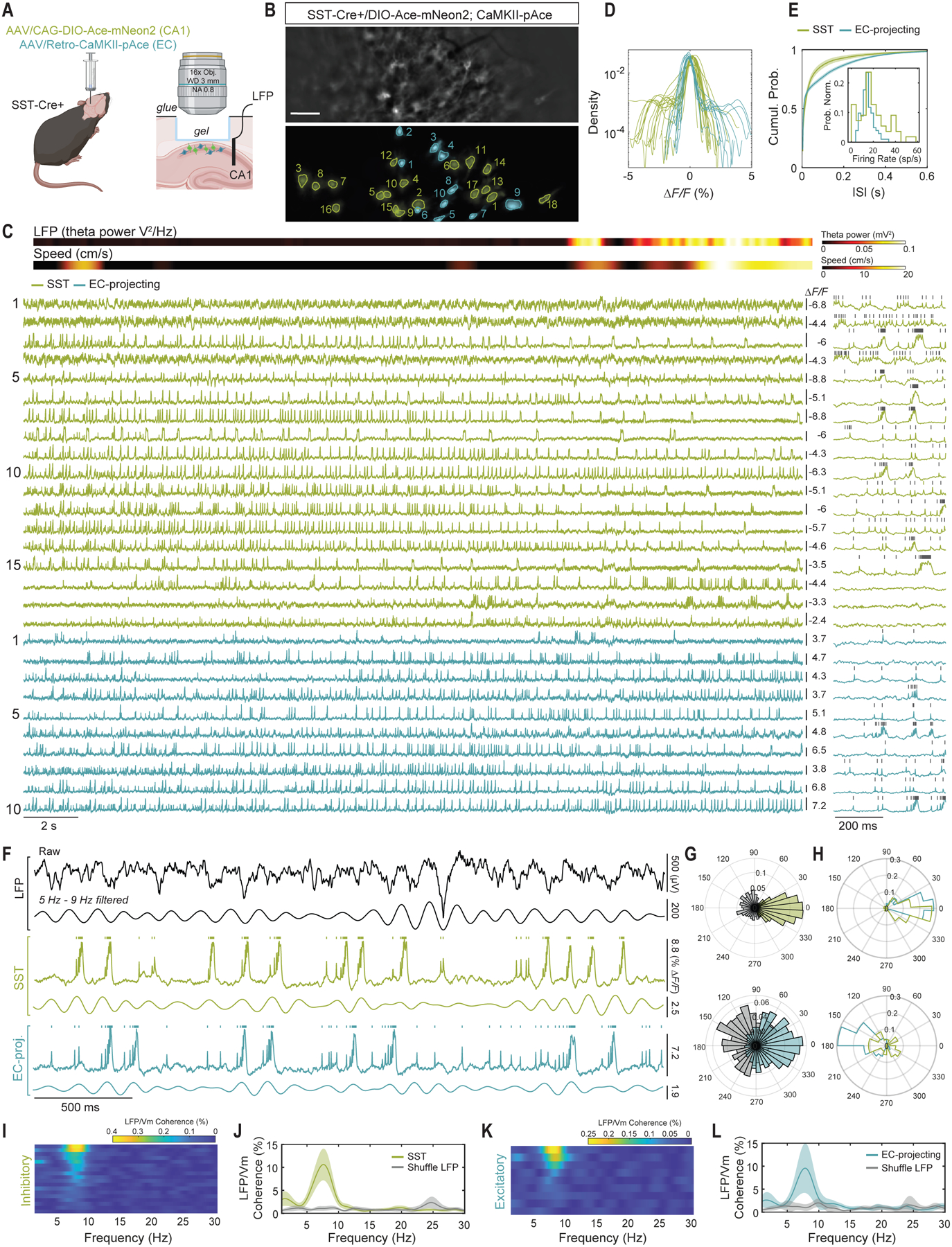
(A) Schematic of AAV injections and experimental setup.

(B) Representative raw epifluorescence image (top) and spatial footprint of negative- and positive-polarity signals (in green and blue, respectively) of 18 and 10 identified neurons. Scale bar: 50 μm.

(C) ΔF/F traces for all the neurons in (B) along with wheel speed and LFP theta (top). Ace-mNeon2 traces are inverted for visualization purposes. The first 500 ms are shown at the expanded timescale to the right. Grey ticks denote identified spikes.

(D) Time course distribution of all neurons across all fields-of-view. Note the opposite polarities within similar dynamic ranges for Ace-mNeon2 and pAce.

(E) Cumulative distribution of inter-spike interval and firing rate (inset) for all recorded neurons (n=55 SST⁺ interneurons and 102 projection neurons, 6 fields-of-view, 1 mouse). Shaded area: 95% CI.

(F) Phase relationships between spike and theta oscillations extracted from the LFP or cellular transmembrane voltage oscillations, for projection neurons and SST⁺ cells recorded simultaneously. Shown here, raw LFP trace (top), theta-filtered (5 Hz-10 Hz) (center) and unfiltered excitatory and inhibitory traces (bottom).

(G) Spike-theta phase relationship for the two neurons in (F). Color and gray represent theta V_m and theta LFP, respectively. Note that both neurons are phase-locked to their own V_m and to the LFP but with approximately opposite phases.

(H) Polar histogram of the probability density of the average spike-theta phase relationship for all 157 neurons, computed against their respective theta V_m (top) or theta LFP (bottom). For each neuron, average spike timing relative to theta cycle was computed using the circular mean.

(I-L) LFP-subthreshold coherence of all neurons in (C), showing that a fraction of (I-J) SST⁺ interneurons and (K-L) EC-projecting excitatory neurons are phase-locked to theta LFP. (I and K) Raster plots sorted in decreasing order of theta-band coherence strength. (J and L) LFP coherence averaged across all neurons in (I and K). Shaded area: 95% CI.

SST⁺ interneurons had greater baseline spike rates and burstiness than the EC-projecting neurons (19.8 ± 1.8 Hz versus 14.7 ± 0.5 Hz (mean ± S.E.M.), P<0.01) (Fig. 4E). We assessed the extent to which spiking by the excitatory and inhibitory neurons was phase-locked to membrane potential oscillations in these specific cell types or to CA1 LFP signals. Across a total of 157 neurons, spiking from both cell types was locked with greater precision to intra-population subthreshold oscillations than to the LFP; notably, SST⁺ cells and EC-projecting PNs spiked at distinct phases of their intrinsic theta (4–9 Hz) membrane potential dynamics [13.8 ± 2.6° and – 1.3 ± 4.8°, respectively (mean ± S.E.M., P<0.01)] (Fig. 4, F–H). Spiking in EC-projecting- but not SST⁺ cells also consistently phase-locked to the LFP (P<0.001 and P=0.82, respectively) (Fig. 4, G and H).

We next assessed the relationships between the LFP and the cell type-specific subthreshold dynamics, as well as those between the subthreshold dynamics of the two neuronal classes. We found strong subthreshold coherence between both cell types and the LFP in the theta frequency band (P<0.0001 and P<0.0001, respectively) (Fig. 4, I–L, and S24, A–D). We also found strong intra- and inter-population coherence in the beta frequency band (15–25 Hz) (fig. S24, E–H), in contrast to the lack of beta frequency band coherence with the LFP (fig. S24, A–D).

DUPLEX imaging in live flies

To showcase the use of DUPLEX for multi-cell type recordings across species, we expressed pAce in GABAergic MBON-γ1pedc>ɑ/β neuron and Ace-mNeon2 in the PPL1-α′2α2 dopaminergic neuron in fruit flies (fig. S25A). Both these cells receive excitatory olfactory inputs from mushroom body Kenyon cells, and MBON-γ1pedc>ɑ/β also exerts feedback inhibition onto PPL1-α′2α2 axons (66). When we exposed the double-labeled flies to odorants, DUPLEX imaging of PPL1-α′2α2 axons and MBON-γ1pedc>ɑ/β dendrites revealed that MBON-γ1pedc>ɑ/β was strongly activated throughout exposure to an attractive odor (apple cider vinegar; ACV) but more transiently by a repulsive odor (benzaldehyde; BEN). By contrast, PPL1-α′2α2 was strongly inhibited by ACV but weakly excited by BEN, in accord with the known inhibitory connection from MBON-γ1pedc>ɑ/β to PPL1-α′2α2 (fig. S25, B, and C).

Inter-population correlations of spiking dynamics during state transitions

We next used DUPLEX to examine how state transitions affect the interactions between cortical subtypes. In green DUPLEX recordings from NDNF⁺ and VIP⁺ interneurons in layer 1 of V1 (~50–100 μm below the pia), spike rates were uncorrelated across the two populations under baseline conditions (Fig. 5, A–C), and air puff-induced arousal had no impact on this (mean ± S.E.M. correlation coefficients: 0.07 ± 0.02 before air puff versus 0.10 ± 0.03 afterward) (Fig. 5C). To quantify the effects of air puff on the spiking of individual cells, we also computed a spike modulation index from −1 to 1 (Methods). Spiking by NDNF⁺ and VIP⁺ cells were significantly positively modulated by air puff (mean ± S.E.M.; median values: 0.27 ± 0.02; 0.32 (P<0.0001, one sample Wilcoxon signed rank test against zero) and 0.11 ± 0.03; 0.08 (P=0.006), respectively) (Fig. 5D).

Fig. 5. Dual population recordings in V1 and CA1 during state transitions.

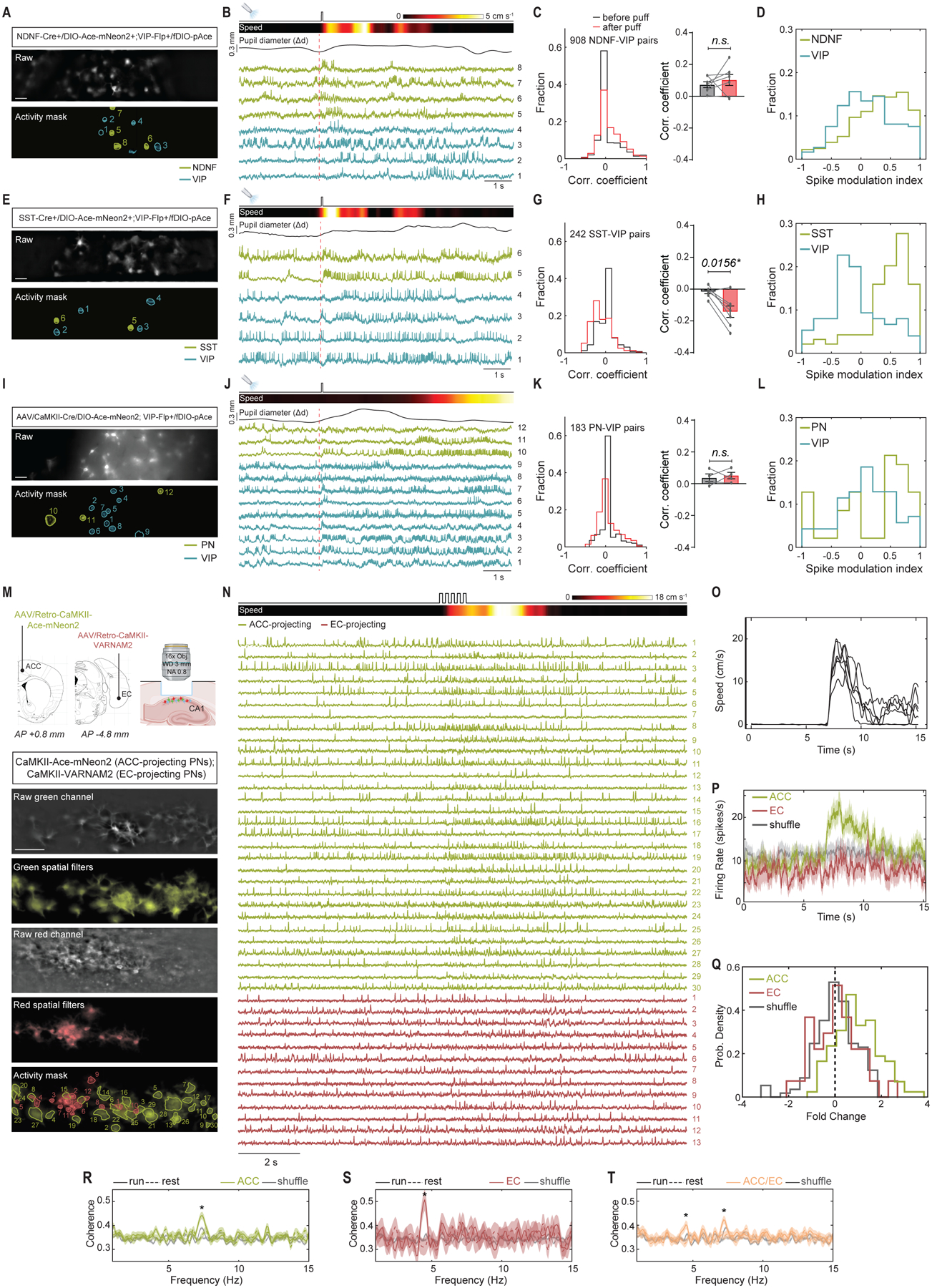
(A-L) DUPLEX recordings in V1.

(A) Representative raw epifluorescence (top) and activity-mask (bottom) images of a single field-of-view from a NDNF-Cre⁺/VIP-Flp⁺ mouse expressing Ace-mNeon2 in NDNF⁺ interneurons (green) and pAce in VIP-cells (blue). Scale bar: 50 μm.

(B) ΔF/F traces from the ROIs numbered in (A) aligned to air puff onset (vertical dashed line). Ace-mNeon2 traces are inverted for visualization purposes. Also shown (top), air puff onset, locomotion speed, and pupil diameter.

(C) Left, Distribution of pairwise inter-class correlation coefficients of spike rates determined using a 20 ms sliding window, for a 3 s-interval before (black) or after (red) air puff (n=908 NDNF-VIP pairs from 393 NDNF⁺ and 188 VIP⁺ cells, 7 mice). Right, Mean ± S.E.M. correlation coefficients by mouse (n=7 mice, n.s.=not significant, One-tailed Wilcoxon matched-pairs signed rank test).

(D) Distribution of spike modulation indices for all NDNF⁺ and VIP⁺ neurons in (C).

(E-G) Same as (A-C) for DUPLEX recordings in SST-Cre⁺/VIP-Flp⁺ mice (n=242 SST-VIP pairs from 103 SST⁺ and 79 VIP⁺ cells, 6 mice, *P<0.05, One-tailed Wilcoxon matched-pairs signed rank test).

(H) Same as (D) for all SST⁺ and VIP⁺ neurons.

(I-K) Same as (A-C) for DUPLEX recordings in AAV-CaMKII-Cre/VIP-Flp⁺ mice (n=183 PN-VIP pairs from 75 PNs and 67 VIP⁺ cells, 4 mice, n.s.=not significant, One-tailed Wilcoxon matched-pairs signed-rank test).

(D) Same as (D) for all PNs and VIP⁺ neurons.

(M-T) Dual-color voltage recordings from hippocampal projection neurons.

(M) Top, Schematic of the experimental approach. Bottom, Representative field-of-view of the red and green channels in grayscale, their respective overlay of spatial filters estimated by EXTRACT for each spiking neuron in each spectral channel, and the overlay of the spatial filter contours for all 30 and 13 identified, projection specific neurons, respectively. Scale bar: 50 μm.

(N) ΔF/F traces for all neurons in (M), aligned to the rest-run transition. Also shown (top), the onset of 5 consecutive air puffs and wheel speed.

(O) Average mouse speed for 5 trials (black). Individual trials are shown in grey.

(P) Average firing rate (250 ms window) for each projection-specific class. Shuffle is computed by random circular permutations of each neuron’s spike train. Shaded area: 95% CI.

(Q) Fold-change in cells’ spiking rates, computed across 2 s-intervals before and after air puff. Shuffle is computed using a random circular permutation of each neuron’s spike train.

(R-T) Average pairwise coherence of the subthreshold dynamics of neurons belonging to the ACC-projecting subclass (R; n=101 neurons); the EC-projecting subclass (S; n=34 neurons); and across the two subclasses (T; n=135 neurons, 5 fields-of-view, 1 mouse). *P value<0.0001 (rank-sum test computed during epochs of running, against levels estimated from neurons belonging to different fields-of-view). Shaded areas represent 95% CI.

In DUPLEX recordings from SST⁺ and VIP⁺ interneurons (~200–250 μm below the pia), spiking by the subtypes became significantly more anti-correlated after air puff (mean ± S.E.M. correlation coefficients: −0.02 ± 0.01 before air puff versus −0.14 ± 0.03 afterward) (Fig. 5, E–G). The spike modulation indices also revealed that most SST⁺ cells were positively modulated by the air puff (mean ± S.E.M.; median values: 0.43 ± 0.05; 0.57 (P<0.0001, one sample Wilcoxon test), whereas VIP⁺ cells imaged concurrently at the same tissue depth and in the same fields-of-view more commonly had negative values of the spike modulation index (mean ± S.E.M.; median values: −0.07 ± 0.05; −0.12 (P=0.14) (Fig. 5H).

DUPLEX studies in PNs and VIP⁺ cells (~150–200 μm below the pia) revealed uncorrelated dynamics for these cell classes before and after air puff (mean ± S.E.M. correlation coefficients were: 0.04 ± 0.02 before versus 0.05 ± 0.02 after air puff) (64) (Fig. 5, I–K). The spike modulation indices revealed a small positive modulation of both cell classes by the air puff (mean ± S.E.M.; median values: 0.19 ± 0.09; 0.44 (P=0.06, one sample Wilcoxon test) and 0.08 ± 0.05; 0.07 (P=0.14), respectively) (Fig. 5L).

Dual-color voltage imaging of hippocampal projection neurons

While DUPLEX can dissect activity patterns among non-overlapping populations, such as discrete excitatory and interneuron subtypes, when the level of overlap between two neuron classes is unknown, the two can instead be monitored by simultaneous dual-color voltage imaging. We used Ace-mNeon2 and VARNAM2 to examine the extent to which two subsets of CA1 projection neurons, targeting distinct cortical regions, modulate their spiking during a rest-to-run behavioral transition. We expressed Ace-mNeon2 and VARNAM2 in anterior cingulate cortex (ACC)- and EC-projecting CA1 pyramidal neurons, respectively, via retrograde AAV labeling. We then performed simultaneous dual-color voltage imaging in an injected mouse, head-restrained on a running wheel, and used a brief air puff to elicit a rest-to-run behavioral transition (Fig. 5M).

We imaged a total of 101 ACC- and 34 EC-projecting neurons from 5 fields-of-view in the same animal, with a single field-of-view containing as many as 30 and 13 cells of the two subpopulations, respectively (Fig. 5, M–N, and fig. S26). Both Ace-mNeon2 and VARNAM2 captured a diversity of cell dynamics, including isolated spikes, spike bursts, and subthreshold oscillations.

We assessed whether the ACC- and EC-projecting cell ensembles had distinct supra- and subthreshold dynamics across the behavioral state transition (6–9). While EC-projecting cells did not significantly change their spike rates after the onset of locomotion, ACC-projecting cells did (log2 fold change (mean ± S.E.M.): 0.0 ± 0.2 for EC-projecting versus 0.9 ± 0.1 for ACC-projecting cells, P=0.59 and P<0.0001; rank-sum test between real data and spike trains circularly permuted in time) (Fig. 5, M–Q, and fig. S24). We also observed greater coherence in subthreshold activity after the behavioral transition, but, interestingly, each subclass synchronized at distinct frequencies (7.3 ± 0.3 Hz and 4.2 ± 0.2 Hz, respectively, for ACC- and EC-projecting cell pairs, P<0.0001, rank-sum test computed for run epochs, against levels estimated from neurons belonging to different fields-of-view) (Fig. 5, R–T).

Simultaneous voltage imaging of three cell populations

Together, our indicators enable discriminations of cell type based on the polarity of optical spike waveforms as well as spectral orthogonality. Thus, in principle, the four GEVIs are mutually compatible and allow recordings from up to four distinct neuron-types at once. To demonstrate dual polarity and dual-color multiplexing, we performed proof-of-concept voltage imaging from three distinct cell classes simultaneously.

In an SST-Cre⁺/VIP-Flp⁺ double transgenic mouse, we injected AAVs encoding both Cre-dependent Ace-mNeon2 and Flp-dependent pAce into V1, plus a retrograde AAV expressing CaMKII-VARNAM2 in area AM to label a subset of excitatory projection neurons (Fig. 6A). We then performed voltage imaging using dual-color, widefield epifluorescence microscopy to record from SST⁺, VIP⁺, and excitatory cells concurrently (Fig. 6, B and C).

Fig. 6. Simultaneous dual-polarity and dual-color imaging capture the voltage dynamics of three distinct cell classes in awake mice.

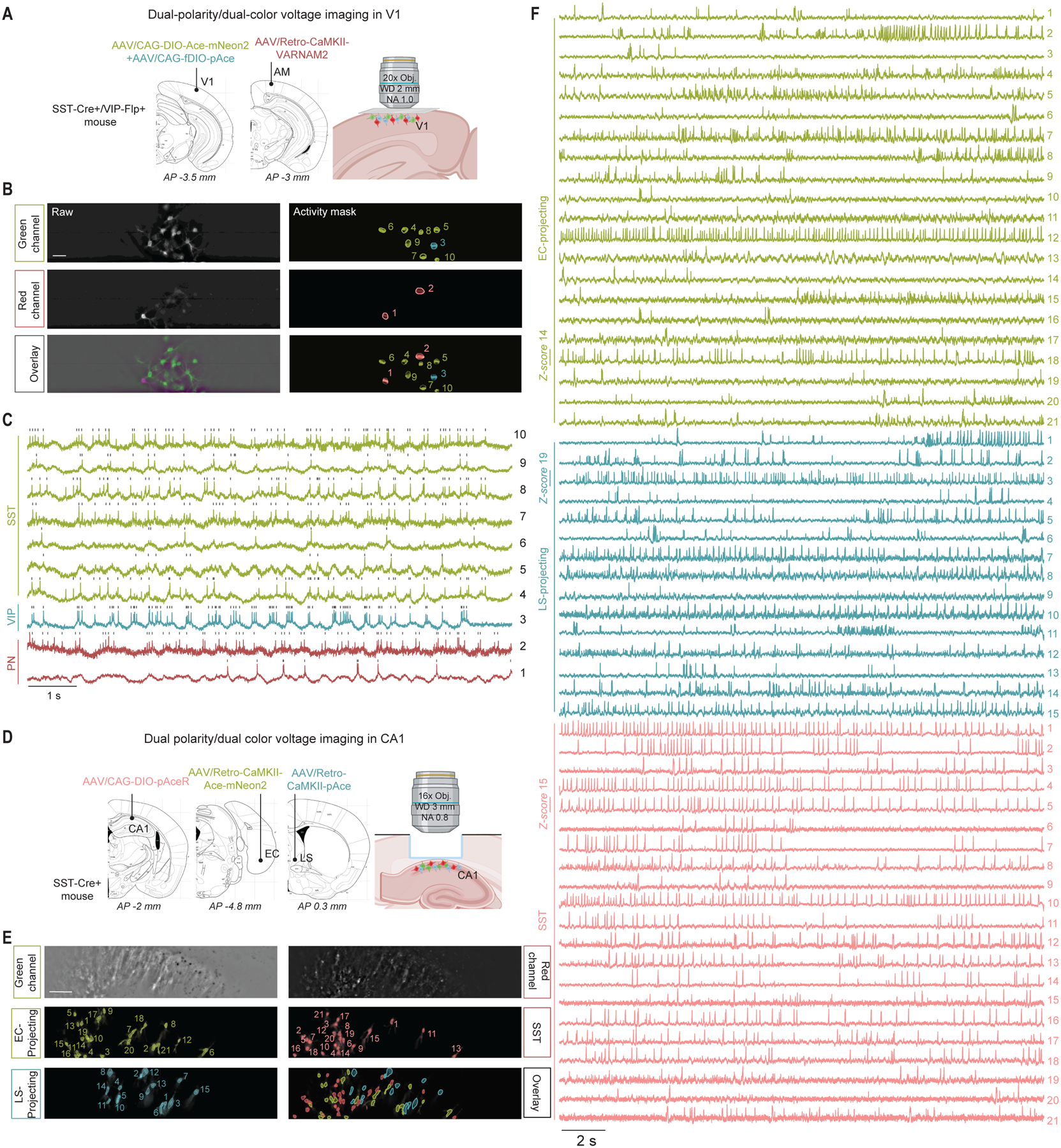
(A) Schematic of AAV injections for three cell class V1 imaging.

(B) Raw epifluorescence (left) and activity-mask (right) images of a single field-of-view in the green and red channels, and overlay. Scale bar: 50 μm.

(C) ΔF/F traces from the ROIs numbered in the mask overlay image in (B) and representing SST⁺ interneurons, VIP⁺ interneurons, and PNs, expressing Ace-mNeon2 (green), pAce (blue), and VARNAM2 (dark red), respectively. Ace-mNeon2 and VARNAM2 traces are inverted for visualization purposes.

(D) Schematic of AAV injections for three cell class voltage imaging in CA1.

(E) Representative field-of-view of the red and green channels with the respective spatial footprint of the identified neurons belonging to each of the three cell classes. Scale bar: 50 μm.

(F) ΔF/F traces for all neurons in (E), representing EC-projecting and LS-projecting excitatory neurons, and SST⁺ interneurons expressing Ace-mNeon2 (green), pAce (blue), and pAceR (pale red), respectively. Ace-mNeon2 traces are inverted for visualization purposes.

To image three neuron classes at once in hippocampus, we retrogradely labeled EC- and lateral septum (LS)-projecting CA1 pyramidal neurons, as well as SST⁺ interneurons, using viruses to express Ace-mNeon2, pAce, and pAceR, respectively, in a SST-Cre⁺ mouse (Fig. 6D). With simultaneous dual-color imaging, we captured the concurrent spiking and subthreshold activity of as many as 57 cells in one field-of-view belonging to the 3 subpopulations (21 EC-projecting, 15 LS-projecting, and 21 SST⁺ cells). These ensembles comprised non-overlapping cell populations (Fig. 6E), and all three GEVIs reported spiking at high signal-to-noise ratios (Fig. 6F).

Conclusion

Our suite of mutually compatible GEVIs allows simultaneous high-speed voltage imaging of multiple genetically identified ensembles in awake animals. Notably, our indicators can provide large datasets for quantitative characterizations of the spiking patterns of targeted neuron classes in behaving flies and mice. This provides a starting point for future studies in which the fine-scale dynamics between targeted cell classes can be examined towards dissecting the circuit basis of animal behavior. The FRET-opsin GEVIs introduced here are bright and can be used with illumination levels far lower than those needed for imaging opsin GEVIs (16, 22, 23, 27). They are hence compatible with both widefield epifluorescence microscopy and specialized microscopy methods that use sculpted illumination patterns (16, 22, 24), facilitating broad dissemination of our voltage imaging approaches.

Our V1 data, acquired from ~1200 cells using Ace-mNeon2, reveal that SST⁺ interneurons exhibit a major increase in spontaneous firing during arousal, recapitulating the results of targeted patch recordings (4). While our results do not confirm the VIP⁺ neuron-centered PN disinhibition model (VIP ⊣ SST ⊣ PN), which was proposed based on Ca²⁺ imaging data (2, 67, 68), the distinct findings might stem from key experimental differences, such as the presence or absence of visual stimuli (69). However, past interpretations of Ca²⁺ imaging data might be confounded by subclass-specific differences in intracellular Ca²⁺ dynamics or cytosolic Ca²⁺ release, which in turn may be influenced by state-dependent neuromodulatory effects (69). A prior alternative to Ca²⁺ imaging was to perform targeted whole-cell patch electrode recordings, but the invasiveness of the technique and the availability of fewer healthy cells for successful patching makes it challenging to sample large numbers of cells from sparse populations (e.g., VIP⁺ interneurons) (2). The use of GEVIs avoids such limitations of electrodes and Ca²⁺ imaging, and our suite of 4 compatible GEVIs enables unprecedented studies of spiking in multiple identified neuron classes at once.

Notwithstanding, our imaging methodology does have limitations. Our widefield one-photon epifluorescence imaging studies in the mouse neocortex, like other recent voltage-imaging studies (13, 16, 23, 24), were limited to supragranular cortical layers, relatively sparse fluorescence labeling patterns, and moderately sized fields-of-view. Similarly, our studies of the CA1 hippocampal area were limited to its two most superficial layers. In these regions, by combining high brightness indicators with cell-type specific and soma-targeted labeling strategies, we achieved high signal-to-background fluorescence and d’ values for accurate spike detection and timing estimation (fig. S18), independent of the cell extraction algorithm used (fig. S15, B, D, and G).

To access cells in deeper cortical layers, the use of patterned illumination strategies to reduce background fluorescence may improve imaging depths (16, 22, 24, 70). Alternatively, imaging of voltage dynamics in infragranular cortical layers or deep brain areas via a microprism (71) or gradient index (GRIN) microendoscope (72) should also be feasible, especially using high numerical aperture lenses (73) for enhanced fluorescence collection than those typically used for Ca²⁺ imaging (74). Further, while the densities of labeled cells in our recordings (<370 cells mm⁻²) were comparable to those of past voltage-imaging studies (13, 16, 22, 23), they were low compared to the total neuronal density in the mammalian cortex. Thus, our imaging approach may not generalize to studies requiring pan-neuronal or other dense labeling strategies. That said, recent work has aimed to delineate the large number of mammalian neuron-types in cortex (75), so we expect that upcoming studies seeking to differentiate the functional attributes of these distinct cell-types will require targeted labeling strategies as those used here. With continued progress in scientific-grade image sensor chips, we also expect improved high-speed cameras that will enable voltage imaging over larger fields-of-view and of more cells than those studied here.

We quantified the veracity of optically detected spike trains using the d’ metric, but measuring the fidelity of optically detected, subthreshold membrane potential changes is more challenging, because the relevant fluorescence signals and noise fluctuations are not just frequency-dependent but also non-stationary. Although the subthreshold components of the estimated neural activity traces, ΔF/F (t), did vary to a modest extent with the use of different cell extraction algorithms (fig. S15), likely due to different efficacies in computationally removing background fluorescence contaminants or heartbeat artifacts, the biological conclusions obtained about cell class interactions using spike rate correlations and subthreshold correlations were in general agreement with each other (Fig. 3, I, K, and M) and did not depend on the analytic approach to cell extraction (fig. S22). Nonetheless, further progress in cell extraction algorithms that are tailored for voltage imaging studies remains important.

Traditionally, multipopulation imaging has been achieved using spectrally orthogonal indicators (18, 59–62). Yet, likely due to the limited set of mutually compatible sensors or the need for tailored optical hardware, simultaneous multichannel imaging is not widely performed in live animals. DUPLEX offers a simple alternative to distinguish two cell classes using one fluorescence channel. Here, DUPLEX unveiled anti-correlated dynamics among pairs of visual cortical SST⁺ and VIP⁺ interneurons during arousal. In hippocampus, DUPLEX revealed cell class-specific subthreshold activity, which allowed us to characterize how the dynamics of excitatory and inhibitory populations relate to those of the LFP. Our results fit with the hypothesis that excitatory neurons contribute more strongly to the LFP due to their spatial organization and temporal synchronization (76).

While DUPLEX allows recordings from non-overlapping cell classes, our green and red indicators can be combined for studies of two cell populations that overlap, or for which the degree of overlap is unknown. The ACC- and EC-projecting CA1 ensembles represent spatially distinct subpopulations, as seen from the non-overlapping expression of Ace-mNeon2 and VARNAM2 (Fig. 5M). This anatomical distinction and the separate dynamical attributes of the two cell classes (Fig. 5P–T) are in line with the idea that there are heterogeneous parallel modules in hippocampus (77).

Looking ahead, that our two green GEVIs of opposite polarities can be further combined with our red GEVIs should enable many different voltage-imaging studies of 3 or 4 cell classes simultaneously (Fig. 6). Thus, the new indicators collectively empower neuroscientists to unravel intercellular interactions within and between targeted neuron classes in awake behaving animals.

Materials and Methods

Plasmids

For high-throughput screening in HEK cells, VARNAM and Ace-mNeon were inserted in a modified pCAGGS backbone (18). A nuclear localization sequence (NLS)-tagged FP reporter (mCerulean for VARNAM and mCherry for Ace-mNeon) was fused to the C-terminus of the indicator interspersed by a T2A ribosomal skipping signal. For in vivo voltage imaging, the indicators were cloned in adeno-associated viral (AAV) backbones. pAAV-CaMKII-Ace-mNeon2, pAAV-CaMKII-VARNAM2 and pAAV-CaMKII-pAce were cloned by inserting the respective indicator sequences in place of EGFP between the KpnI and HindIII sites of pAAV-CaMKII-EGFP (Addgene #50469). Cre-dependent constructs for Ace-mNeon2 and pAceR were generated by cloning the respective inverted open reading frame (ORF) sequences in pAAV-CAG-Flex-EGFP (Addgene #59331) by replacing the floxed EGFP cassette between the AscI and NheI sites. Likewise, Flp-dependent VARNAM2 and pAce constructs were cloned by introducing the respective inverted ORF sequences in place of the floxed mNeonGreen between the AscI and NheI sites in pAAV-CAG-fDIO-mNeonGreen (Addgene #99133). All AAV constructs above included a Golgi/ER export sequence and a Kv2.1 proximal restriction and clustering sequence (43) at the C-terminus of the indicator sequence for improved membrane trafficking and perisomatic localization, respectively.

Fly stocks

To create transgenic flies carrying the four improved FRET-opsin GEVIs, we synthesized codon-optimized transcripts for Ace-mNeon2, VARNAM2, pAce and pAceR using a commercial gene synthesis service (GenScript), and then inserted them in place of GFP in the pJFRC7-20×UAS-IVS-mCD8::GFP (Addgene #26220) and pJFRC19-13×LexAop2-IVS-myr::GFP backbones (Addgene #26224). After verifying the sequences of the plasmids, we inserted the plasmids into the attP40 or VK00027 phiC31 docking site to generate 20×UAS-Ace-mNeon2, 13×LexAop-Ace-mNeon2, 20×UAS-pAce, 13×LexAop-pAce, 20×UAS-VARNAM2, 13×LexAop-VARNAM2, 20×UAS-pAceR and 13×LexAop-pAceR flies using a commercial transformation service (Bestgene Inc.).

We obtained MB058B, MB296B, and MB085C split-GAL4 lines from the FlyLight team at Janelia Research Campus, and R82C10-LexA (#54981) from the Bloomington Stock Center. We raised all flies on standard cornmeal agar media under a 12 h light/dark cycle, at 25°C and 50% relative humidity.

Site-directed saturation mutagenesis

Mutagenic libraries were generated on Ace-mNeon-T2A-NLS-mCherry and VARNAM-T2A-NLS-mCerulean backbones using a pre-established protocol (18). Briefly, a set of 4 forward primers, containing degenerate codons WKC, NMC, VWG, or DGG at the target site, was pooled with a single, partially overlapping reverse primer, and mutagenizing PCR reactions were set up using CloneAmp^™ polymerase (Clontech). Following DpnI treatment to digest unmutated template, the linear PCR products were circularized using InFusion^® ligase (Clontech) and transformed in TOP10 competent cells (Invitrogen). To obtain up to 19 unique AA substitutions at a single target site, 48 colonies were picked and cultured in 96 deep-well culture plates. Plasmid DNA was isolated using Nucleospin^® 96 Plasmid kit (Macherey-Nagel) on an epMotion 5075 liquid handling workstation (Eppendorf), and purified DNA was collected in 96-well plates. The libraries were sequenced after voltage screening to identify the individual mutations and ensure at least 19 variants were obtained at every site.

Maintenance and transfection of HEK and excitable HEK cells

HEK293 cells (ATCC^® CRL-1573^™) were maintained in high-glucose DMEM/10% FBS. Excitable HEK cells (ATCC^® CRL-3269^™) (30, 31) were maintained in DMEM/F12, 10% FBS, 1% penicillin (100 U ml⁻¹), streptomycin (100 μg ml⁻¹), geneticin (500 μg ml⁻¹), and puromycin (2 μg ml⁻¹) as described previously. ~24 h prior to transfection, the cells were plated on poly L-lysine-coated 12 mm coverslips or 96-well glass-bottomed plates in antibiotic-free media. Plasmid DNA (0.5 μg/12 mm coverslip or 0.2 μg/well of a 96-well plate) was transfected using Lipofectamine^® (ThermoFisher), and cells were imaged 1–2 d post-transfection. Both cell lines served solely as a system for the expression and characterization of voltage indicators rather than the subject of investigation.

High-throughput semi-automated voltage screening

High-throughput voltage screening (Fig. 1B) was performed on a custom-built platform described previously (18). A white light source pE-4000 (CoolLED, UK) was used for sample illumination. For imaging Ace-mNeon, we used a 472/30 nm excitation filter, 495 nm dichroic mirror, and 520/35 nm emission filter (Semrock). For VARNAM and mCherry (reporter fluorophore in Ace-mNeon constructs), we used a 560/40 nm excitation filter, 585 nm dichroic mirror, and 630/75 nm emission filter (Chroma Technologies Corporation). mCerulean reporter in the VARNAM constructs was imaged using a 455/40 nm excitation filter, 458 nm dichroic mirror, and 480/30 nm emission filter (Semrock). After identifying transfected cells in the reporter channel, time-series fluorescence images were captured in the respective GEVI channels using ORCA Flash4.0 sCMOS camera (Hamamatsu) at 50 Hz. A single pulse of 60 V/0.5 ms was applied using a Grass S48 Stimulator, 1 s after baseline fluorescence acquisition (F₀). % change in fluorescence at time t was obtained using the formula

$$\frac{\Delta \mathit{F}}{{\mathit{F}}_{\mathbf{0}}}\%=\frac{F(t)-F_{\mathbf{0}}}{F_0}\times 100$$

Platform automation, sample illumination, data acquisition and parallel data analysis were controlled using custom-written virtual instruments in LabView^®.

Fluorescence voltage imaging in cultured HEK cells

Whole-cell voltage-clamp recordings were performed between 22–25°C. The bath solution contained (in mM): 125 NaCl, 2 KCl, 10 HEPES, 30 glucose, 3 CaCl₂, 1 MgCl₂ (~310 mOsm l⁻¹, pH 7.3). The intracellular solution consisted of (in mM): 125 K-gluconate, 8 NaCl, 0.6 MgCl₂, 0.1 CaCl₂, 1 EGTA, 4 Mg₂-ATP, 0.4 Na-GTP and 10 HEPES. Patch pipettes had tip resistances of 4–5 MΩ, yielding series resistances <20 MΩ. In the voltage-clamp mode, voltage steps in increments of 20 mV/ 0.5 s were applied via a MultiClamp amplifier controlled by pClamp10 software.

Fluorescence recordings were obtained using an Olympus upright microscope. Cells were visualized under a 1.0 NA 60x water-immersion objective lens. Ace-mNeon and pAce were imaged using a 505 nm light-emitting diode (LED) (Thorlabs) and a filter set comprising 509/22 nm excitation filter, 526 nm dichroic mirror and 544/24 nm emission filter (Semrock). VARNAM and pAceR were illuminated using a 565 nm LED (Thorlabs), 560/40 nm excitation filter, 585 nm dichroic mirror and 630/75 nm emission filter (Semrock). The illumination intensity at the sample plane for all indicators was 15–20 mW mm⁻². Fluorescence time-series images (1–5 kHz) were captured using a NeuroCCD camera, controlled via NeuroPlex software (RedShirtImaging, GA). Fluorescence response traces were extracted by ranking each pixel by their signal-to-noise ratios, where the noise was calculated as the root mean square value of the baseline fluorescence fluctuations. The top 25% of the SNR-ranked pixels were used to calculate the ΔF/F values shown in Fig. 1D and fig. S5. Probe kinetics for activation (τ_ON) and deactivation (τ_OFF) were calculated from 5 kHz recordings obtained in HEK cells, by fitting the first 50 ms of the step responses using a double exponential equation as described previously (78).

Surgical dissection of live flies

We created an optical window on the fly head using an ultraviolet (UV) laser microsurgery system, as described previously (79). In brief, we anesthetized the flies by placing them on ice for 1 min and then transferring them to a cooled surface (~4 °C) consisting of an aluminum thermoelectric cooling block. We then glued the fly’s thorax with a 125 μm-diameter fused silica optical fiber (PLMA-YDF-10/125, Nufern) on a custom-made plastic fixture. To minimize head motion, we glued the fly’s head to the thorax using a UV light curing epoxy (NOA 89, Norland). After transferring the mounted fly to the surgery station, we created an optical window in the cuticle by laser-drilling a 150-μm-diameter hole (30–4¬0 pulses, delivered at 100 Hz, 36 mJ per pulse, as measured at the specimen plane). Immediately after surgery, we applied 1 ml of UV epoxy (NOA 68, Norland; Refractive index: 1.54; Transmission 420–1000 nm: ~100%) and cured it for ~30 s to seal the cuticle opening.

Visual cortical surgeries

Animal experiments were performed according to the guidelines of the National Institutes of Health and approved by The John B. Pierce Laboratory Animal Care and Use Committee.

Intracranial AAV injections.

C57BL/6J wild-type and VIP-Cre, SST-Cre, VIP-Flp, and NDNF-Cre transgenic mice were purchased from The Jackson Laboratory (JAX #664, #31628, #13044, #28578, #28536). NDNF-Cre^+/+ or SST-Cre^+/+ mice were crossed with VIP-Flp^+/+ to generate the NDNF-Cre⁺/VIP-Flp⁺ and SST-Cre⁺/VIP-Flp⁺ double driver lines. The following AAV vectors were custom-produced at the University of North Carolina Vector Core at high titers (>1 × 10¹³ GC ml⁻¹): AAV/DJ-CAG-DIO-Ace-mNeon2, AAV2/Retro-CaMKII-Ace-mNeon2, AAV/DJ-CAG-fDIO-pAce, AAV2/Retro-CaMKII-pAce, AAV/DJ-CAG-fDIO-VARNAM2, AAV2/Retro-CaMKII-VARNAM2, and AAV/DJ-CAG-DIO-pAceR. All AAV vectors above encode soma-targeted versions of the indicators. AAV5-CaMKII-mCherry-Cre and AAV2/Retro-EF1A-mCherry-IRES-Cre viruses were purchased from the UNC Vector Core and Addgene (#55632), respectively.

Mice were used without regard to sex; we used a total of 21 males and 23 females in this study. Stereotactic AAV injections were performed in 3–4 month-old mice under 1.5% (v/v) isoflurane anesthesia. The coordinates for V1 injections in Fig. 1, H–K; Fig. 2; Fig. 3; Fig. 5, A–L; and Fig. 6, A–C, as well as supplementary fig. S16, S17, S19, and S21 were (in mm from Bregma; AP, ML): 2.5, 2.5; 2.8, 2.0; 3.0, 2.5; 3.4, 2.0; 3.6, 2.75; DV=0.2–0.3. For PN projection labeling in the anteromedial (AM) visual cortical area (Fig. 1J; Fig. 2E; fig. S21), the coordinates were (AP, ML, DV): 3.0, 0.96, 0.4. Injections were performed using beveled glass micropipettes delivering a total of 50–100 nl virus/site at a rate of 100 nl/min.

For targeted recordings from identified cell classes (Fig. 1, H–K; Fig. 2; fig. S16, S17, S19), AAV/DJ-CAG-DIO-Ace-mNeon2 (or AAV/DJ-CAG-fDIO-pAce) was injected in Cre- (or Flp)-recombinase-expressing transgenic driver lines. For DUPLEX imaging (Fig. 3, A-M; Fig. 5, A–H), AAV/DJ-CAG-DIO-Ace-mNeon2 and AAV/DJ-CAG-fDIO-pAce viruses were mixed at a 1:3 (v/v) ratio for injections in NDNF-Cre⁺/VIP-Flp⁺ or at a 1:1 ratio for injections in SST-Cre⁺/VIP-Flp⁺ mice. For DUPLEX recordings from PNs with VIP⁺ interneurons in VIP-Flp⁺ mice (Fig. 3, L, M; Fig. 5, I–L; fig. S21), the AAV/DJ-CAG-DIO-Ace-mNeon2 virus was mixed with the AAV5-CaMKII-mCherry-Cre virus for Ace-mNeon2-labeling of PNs and injected together with an equal volume of the AAV/DJ-CAG-fDIO-pAce virus for pAce-labeling of VIP⁺ interneurons. To lower PN labeling densities by labeling a subset of neurons projecting to a higher-order visual cortical area (Fig. 1J; Fig. 2E), the AAV/DJ-CAG-DIO-Ace-mNeon2 virus was injected locally in V1, while the AAV2/Retro-EF1A-mCherry-IRES-Cre virus was delivered to the AM cortical area.

For dual-color imaging (Fig. 6, A–C), AAV/DJ-CAG-DIO-Ace-mNeon2 and AAV/DJ-CAG-fDIO-VARNAM2 were mixed at a 1:1 (v/v) ratio for injections in an SST-Cre⁺/VIP-Flp⁺ background.

Histology and confocal imaging.

For confocal imaging of the cell-type-specific expression of Acem-Neon2 in area V1 (Fig. 2, B–E, panel a), injected mice were transcardially perfused with ice-cold Sorenson’s buffer (pH 7.4) followed by 4% paraformaldehyde. The brains were isolated and post-fixed overnight at 4°C. 40–60 μm thick coronal sections comprising the visual cortical areas were prepared on a Leica vibratome and mounted on gelatin-coated glass microscope slides using ProlongGold (Invitrogen). Confocal micrographs were obtained using Zeiss LSM 710 under a 20X air objective.

Headpost and cranial window implantation.

Headpost and cranial windows were implanted between 25–30 days post-injection with some modifications to a pre-established protocol (80). Mice were anesthetized using a mixture of ketamine (100 mg/kg) and xylazine (16 mg/kg). A custom-designed titanium head post was affixed to the skull using C&B Metabond (Parkell), following which a 3-mm-diameter circular craniotomy was made over the injection area in V1. A sterile double-glass window, assembled by gluing one each of 3 mm and 5 mm diameter circular coverslips (Warner), was secured in place using Vetbond, as previously described (80). C&B Metabond was applied over the window margins and the remainder of the exposed skull. Carprofen (5 mg/kg, SC, every 24 h for 48 h) and buprenorphine (100 μg/kg, SC, every 12 h for 48 h) were administered as part of postoperative analgesia. Prior to awake imaging experiments, the headposted mice were handled and habituated to run on a custom wheel every day for up to 2 weeks in 10–20 min training sessions. Imaging began once the animal was fully wheel-trained.

Hippocampal CA1 surgeries

The Stanford Administrative Panel on Laboratory Animal Care (APLAC) approved all procedures involving animals, and we complied with all ethical regulations.

Hippocampal AAV injections.

C57BL/6J wild-type and SST-Cre transgenic mice were purchased from The Jackson Laboratory (JAX #664 and #013044). Mice (aged 8–16 weeks at start) underwent two surgical procedures under isoflurane anesthesia (1.5%–2% in O₂). In the first procedure, we injected AAVs to express the fluorescent voltage indicators. In the second procedure, performed about a week after viral injection, we inserted a cannular implant for hippocampal imaging.

The coordinates for CA1 injections in Fig. 4; Fig. 6, D–F; and fig. S23–24, were (in mm from Bregma; AP, ML, DV) −1.8, −2.5, −1.1 and −1.3, −1.3, −1.1. The coordinates for retrograde labeling in the lateral septum (LS) (Fig. 6, D–F), entorhinal cortex (EC) (Fig. 5, M–T; Fig. 6, D–F; fig. S23–24, 26) and anterior cingulate cortex (ACC) (Fig. 5, M–T; fig. S26) were, respectively, (in mm from Bregma; AP, ML, DV): 0.3, 0.3, −3; −4.8, 3.3, −3.5 and 0.8, 0.2, −1.5. We used the following viruses: AAV/DJ-CAG-DIO-Ace-mNeon2 and AAV2/Retro-CaMKII-pAce to label SST neurons and EC-projecting neurons, respectively (Fig. 4); AAV2/Retro-CaMKII-VARNAM2 and AAV2/Retro-CaMKII-Ace-mNeon2 to label EC-projecting and ACC-projecting neurons, respectively (Fig. 5); AAV2/Retro-CaMKII-Ace-mNeon2, AAV2/Retro-CaMKII-pAce, and AAV/DJ-CAG-DIO-pAceR to label EC-projecting and LS-projecting neurons, SST-neurons, respectively (Fig. 6); and AAV/DJ-CAG-DIO-pAceR and AAV2/Retro-CaMKII-VARNAM2 to label SST neurons and EC-projecting neurons, respectively (fig. S23). All viral vectors had titers of >10¹² GC ml⁻¹ and were custom-produced at the UNC Vector Core.

Cannular implant fabrication and preparation of LFP electrodes.

Cannula implants were prepared under a stereomicroscope (Leica MZ7–5) with a fully equipped solder station. The hippocampal cannula consisted of a circular borosilicate cover glass (3 mm diameter, 170 mm ± 5 mm thickness, Schott) glued to the end of a 3 mm OD, 1.5 mm long stainless-steel ring, using UV-curable adhesive (Loctite 3105) (Fig. 5M–T; Fig. 6; fig. S23).

For the dual-modality optical-LFP hippocampal recordings (Fig. 4), we affixed three ~1-cm-long, ~50-μm-diameter tungsten wires coated with single polyimide insulation (M215580, California Fine Wire) to the optical cannula at three different axial positions, spaced in increments of ~50 μm. The tip of one of the three tungsten wires was placed flush with the optical window, and the tips of the other two extended beyond the optical window. This set of electrode placements was chosen to maximize the chances that at least one of the electrodes would provide high-quality LFP signals, given that our surgical placement of the implant was performed without fine visual feedback about the exact location of the ~100-μm thick CA1 pyramidal cell layer. We glued these tungsten wires onto the optical cannula with ultraviolet-light-cured adhesive, which constrained the electrodes to be laterally offset by 1.5 mm from the center of the imaging window. Next, we soldered a gold-plated pinhead (NC0102069, WPI) onto the end of each tungsten wire projecting away from the imaging window. The reference electrode comprised a ~5-mm-long, ~127 μm-diameter, uncoated, stainless-steel wire (#791600, A-M Systems) soldered to a gold-plated pinhead (NC0102069, WPI). Separately, we fabricated a 4-channel-connector using 4 gold-plated sockets (NC1456862, WPI) and a connector board (EIB8, Neuralynx).

Hippocampal cannular implantation.

To implant the optical cannula, we resected the skin and scalp to expose the dorsal surface of the cranium and removed any remaining connective tissue by cleaning the exposed skull with hydrogen peroxide (H₂O₂). To ensure strong adhesion between the cannula implant and the skull, we slightly roughened the skull surface using a drill bit and then rinsed the cranium with Ringer’s solution. We drilled a 3-mm-diameter opening above the right dorsal CA1, sized to allow the cannula implant to fit in snugly. We aspirated the cortex above dorsal CA1 using a 30 G blunt needle, under irrigation with ice-cold Ringer’s solution. We proceeded with cortical aspiration until the light-scattering, myelinated axon bundles of the corpus callosum became visible. Of the 3 superimposed layers of myelinated axons, which were visually distinguishable by their distinct orientations, we removed the top 2 layers with gentle air suction, while making sure to leave intact the stratum oriens layer of hippocampus. (We excluded from further study any mice with surgical damage to CA1, as such damage can lead to local epileptiform activity). The cannula implant was then inserted and affixed to the skull using UV-curable adhesive (Loctite 3105).

For studies in which LFP recordings were to be performed concurrently with imaging, we drilled a 0.5-mm-diameter hole into the skull above the cerebellum, inserted the reference electrode into cerebellar tissue and then affixed it to the skull with UV-curable adhesive (Loctite 3105). Carprofen (5 mg kg⁻¹) was administered 30 min prior to the end of the surgery to mitigate pain. To enable head-fixation during in vivo imaging, we secured a custom stainless steel head bar to the mouse’s skull using blue light-cured resin (Flow-it ALC, Pentron). Carprofen (5 mg kg⁻¹) was administered up to two days post-surgery as part of postoperative analgesia. Mice recovered for ~2 weeks before the start of voltage imaging sessions.

Voltage imaging in awake flies

The fly data was acquired at Stanford University. The optical instrumentation described below was used to obtain the data in Fig. 1, E–G; fig. S13; fig. S14; and fig. S25.

Instrumentation and imaging.

To image voltage dynamics in flies, we used a custom-built upright epi-fluorescence microscope and a 1.0 NA 20X water-immersion objective (XLUMPlanFL, Olympus). For Ace-mNeon and pAce imaging, we used a 503/20 nm excitation filter (Chroma), 518 nm dichroic (Chroma) and 534/30 nm emission filter (BrightLine). We illuminated the sample using the 500-nm wavelength module of a solid-state light source (Spectra X, Lumencor), with 5–7 mW of optical power at the specimen plane. For VARNAM and pAceR imaging, we used a 559/25 nm excitation filter (Semrock), 580 nm dichroic (Chroma) and 630/50 nm emission filter (Semrock). We illuminated the sample using the 550-nm wavelength module of the light source, with 8–10 mW of optical power at the specimen plane. We acquired images at 1000 Hz, using a scientific-grade CCD camera (Zyla 4.2, Andor) and 2 × 2 pixel binning.

Odor delivery.

To image odor-evoked activity, we perfused odors to the flies’ antennae using a custom-built olfactometer that delivered constant airflow (200 ml/min) to either the control path (mineral oil) or the odor path (odorant dissolved in mineral oil). We presented 5% isoamyl acetate (IAA; CAS# 123-92-2, Sigma-Aldrich Inc.), 3% benzaldehyde (BEN; CAS# 100-52-7, Sigma-Aldrich Inc.) or apple cider vinegar (ACV; Bragg Inc.) to the fly via a probe needle (1.7 mm ID, Grainger Inc.), ~3 mm in front of the antenna. Each odor delivery trial lasted for 5 s.

Spike extraction.

To extract the voltage data, we motion-corrected the raw videos using the Turboreg algorithm for image registration (http://bigwww.epfl.ch/thevenaz/turboreg/) (81). We then selected pixels whose mean fluorescence intensity, averaged over the entire movie, was in the top 10% of all pixels across the field-of-view; we defined the union of these high-ranking pixels as the region-of-interest (ROI). We corrected for photobleaching by fitting a double exponential function to the spatially averaged fluorescence across the ROI, F(t), and then dividing F(t) by the fitted double exponential trace. We then computed time-dependent changes in the relative fluorescence intensity, ΔF(t)/F = (F′(t)−F₀)/F₀, where F′(t) was the time-dependent fluorescence intensity trace across the ROI after the photobleaching correction, and F₀ was the time-averaged baseline intensity in the ROI after the photobleaching correction. To identify individual spikes, we high-pass filtered the ΔF(t)/F trace by subtracting a median-filtered (40 ms window) version of the trace and identified spikes as local peaks that surpassed a set threshold (3 S.D. for PPL1-DANs, 2 S.D. for MBON-γ1pedc>α/β). We estimated the instantaneous, time-dependent spike rate by tabulating the number of spikes within a 100-ms sliding window.

To determine the mean spike waveform, we averaged the waveforms of all spikes across a trial. We then performed a spline interpolation (10 μs intervals) of the mean waveform and, from the resultant, determined the spike amplitude and duration. Determinations of the spike detection fidelity for studies in live flies were performed using the same formulae as for studies in mice (see section below, Determinations of the spike detection fidelity index, d′).

Single- and dual-channel voltage imaging in V1 in running mice

All data from brain area V1 (Fig. 1, H–K; Fig. 2, B–E; Fig. 3, A–F; Fig. 5, A–L; and Fig. 6, A–C, as well as figs. S16, S17, S19, and S21) were acquired at the John B. Pierce Laboratory. Prior to the awake animal experiments, head-posted mice were handled and acclimated to a custom 15- cm-diameter 3 D-printed wheel for ~2 weeks in training sessions of 10 min per day.

Instrumentation and imaging.

For in vivo neocortical voltage imaging, mice implanted with cranial windows were head-fixed by securing the head post to two points on the custom wheel via thumbscrews. Neurons expressing soma-targeted indicators at cortical depths of ~50–200 mm below the pial surface (Fig. 2, B–E, subpanel a) were imaged on a custom-built dual-channel upright fluorescence microscope equipped with an epi-illuminator module (WFA2001, Thorlabs), an EYFP/mCherry (59026, Chroma) dual bandpass filter set (comprising a 59026x excitation filter with passbands of 503/12 and 575/15, a 69008bs dichroic mirror with passbands of 470/20, 540/25 and 630/50, and a 59026m emission filter with passbands of 535/15 and 635/35), and a 20X 1.0 NA Olympus XLUMPLFLN water immersion objective.

The illumination from a pair of light-emitting diodes (LEDs), emitting light of 505 nm and 565 nm wavelengths (M505L4 and M565L3, Thorlabs, respectively), was collimated with a pair of aspheric condenser lenses (ACL2520U-A), one for each LED. For dual-channel imaging (Fig. 6, A–C), illumination from the two LEDs was combined using a 550 nm long-pass dichroic mirror (T550 LPXR, Chroma). The illumination intensity at the sample plane in each of the red and green channels was ~25 mW mm⁻².

Fluorescence emissions returning from the sample plane were directed by a 585 nm long-pass dichroic mirror (T585 LPXR, Chroma) into the two fluorescence detection arms of the microscope. Emissions from Ace-mNeon2 and/or pAce passed through a 520/35 nm bandpass filter (FF01–520/35–25, Semrock). Emissions from VARNAM2 and/or pAceR passed through a 630/75 bandpass filter (ET630/75m, Chroma). Within each fluorescence detection arm, a 0.75X camera tube lens (WFA4101, Thorlabs) focused the fluorescence onto a high-speed sCMOS camera (Orca Flash 4.0 v3, Hamamatsu).

For the dual-color, dual-polarity imaging studies of V1 using Ace-mNeon2, pAce, and VARNAM2 in Fig. 6, A–C, both the 505 nm and 565 nm LEDs were ON concurrently, and we acquired data simultaneously from both cameras. For synchronized registration of the images, the two cameras were operated in their external trigger mode, allowing us to trigger image acquisition on both cameras by sending them a single, common TTL pulse. We further verified that image acquisition by the two cameras was synchronized by using the timestamps on the two videos. To ensure that images from the two channels were spatially aligned, we calibrated images against an alignment target to ensure that images were spatially aligned and confirmed this during each imaging session based on reference points e.g., the location of landmark vasculature.

For all experiments in Fig. 1, H–K; Fig. 2, B–E; Fig. 3, A–F; Fig. 5, A–L; and Fig. 6, A–C, as well as figs. S16, S17, S19, and S21, fluorescence time-series images (2048 px × 512 px) were collected at 400 Hz with 4 × 4 binning. We typically acquired 3–4 trials of data from each imaging field-of-view, and we imaged ~6–8 fields-of-view per session. Over the course of several days, but in some cases over 3–4 weeks, we revisited and re-imaged each field-of-view 2–3 more times, using vascular landmarks to identify the approximate tissue locations of prior imaging sessions.

We inferred the cortical depth of the imaged neurons based on the laminar organization, as reported in the published scientific literature, of the different cortical cell classes that we examined. Specifically, we inferred that we recorded neurons in cortical layers 1, 2 and 3 based on published evidence that (i) cortical NDNF⁺ interneurons are layer 1-specific (41, 47, 48), and that (ii) cortical PNs, selectively targeted using CaMKII, and that SST⁺ interneurons, selectively targeted using the published SST-Cre transgenic line (40) are both absent in cortical layer 1. PN projection neurons from the AM area reside in cortical layer 2/3, between 100–200 μm below the pial surface (39, 42). SST⁺ interneurons reside at depths >200 μm beneath the pial surface (40), and VIP⁺ interneurons reside at depths >50–100 μm below the pia (49). Confocal micrographs showing cell class-specific labeling in V1 (Fig. 2, B–E, top panel) further confirmed the laminar organization of the imaged cortical cell classes in the supragranular layers and the relative cortical depths of the distinct neocortical subclasses.

Visual stimulus presentations.

In Fig. 1J, visual stimuli were generated using the Psychophysics toolbox on MATLAB and were presented to awake, stationary mice on an LCD video monitor (1280 × 1024 pixels, 20 × 16 inches, 60 Hz refresh rate, mean luminance of 250 cd m⁻²). The monitor was placed ~15 cm from the animal, perpendicular to the surface of the right eye (contralateral to the injection area). To map the receptive field of an imaged neuron, static bright and dark stimuli were presented individually in a pseudorandom sequence within each square of a 3 × 4 grid extending across the entire video monitor. Once the cell’s receptive field location was approximately mapped, to characterize the cell’s orientation-selective responses, we sequentially presented a set of drifting sinusoidal gratings at one of eight orientations, spaced by increments of 45° and presented in a pseudorandom sequence. The spatial frequency of the grating was 0.04 cycles per division, and the temporal frequency was 2 Hz. Each trial lasted 16 s, with interstimulus intervals of 500 ms.

Induced state transitions and pupillometry.

In Fig. 2, B–E and Fig. 5, A–L, to induce a change of state, a brief 50 ms air puff was delivered to mice at rest using a small tube aimed at the back of the animal. Wheel position was tracked using a programmable angle sensor (KMA210, Digikey). A data acquisition device (NI USB-6259, National Instruments) registered the wheel’s position and delivered TTL pulses to initiate image acquisition. Software code, custom-written in LabView 2019 (National Instruments) controlled data acquisition.

For the state transition experiments in Fig. 2, B–E; and Fig. 5, A–L, an infrared camera (Basler A602f) was used to measure the pupil diameter at a frame rate of 15 Hz. Pupil diameter was measured in real-time using custom code written in LabView. An annulus region-of-interest was drawn over the pupil, with the inner circle located at the center of the eye and the outer circle extending past the edge of the pupil. The edge-detection functionality of the LabView Vision Development Module was used to detect dark-to-light transition points along a set of radial measurement lines drawn from the inner circle and extending to the outer circle. The pupil diameter was calculated by fitting a circle to the set of detected dark-to-light transition points. The threshold level for edge detection and the number of transition points were manually optimized for each individual mouse.

Single- and dual-channel voltage recordings in CA1 in running mice

All imaging studies of hippocampal area CA1 were performed at Stanford University. The optical instrumentation described below was used to acquire the CA1 data shown in Fig. 4; Fig. 5, M–T, and Fig. 6, D–F, as well as figs. S23, S24, and S26.

Instrumentation and imaging.

For green DUPLEX studies (Fig. 4), simultaneous dual-color (Fig. 5, M–T; figs. S24, S26), and triple-population voltage imaging (Fig. 6, D–F), we used a custom-built microscope with a 16X 0.80 NA, 3.0 mm WD, water immersion objective lens (Nikon N16XLWD-PF). For red-DUPLEX (fig. S23), we used a 25X 1.0 NA, 4.0 mm WD, water immersion lens (Olympus XLPLN25XSVMP2). The recording depth for all hippocampal data was ~50–100 μm, as set by the intrinsic cellular organization of the dorsal CA1 area. A motorized stage (Sutter MP-285) was used for fine axial focusing.

Illumination from two light-emitting diodes (LEDs) (UHP-F-470 and UHP-F-545, Prizmatix) was combined using a long-pass dichroic mirror (511 nm, Prizmatix) and then filtered using a dual band-pass clean-up filter (Semrock, FF01–482/563–25, with passbands of 482/18 nm and 563/9 nm). A dual-band dichroic mirror (Semrock, Di01-R488/561–25x36, with passbands of 525/40 nm and 690/108 nm) reflected the combined illumination toward the specimen and transmitted the returning fluorescence emissions. The illumination intensity at the sample plane from each LED was ~25–75 mW mm⁻².

In the emission pathway, to separate fluorescence in the two color channels, we used a 550 nm short-pass dichroic mirror (70 mm × 100 mm, custom-designed, Alluxa) and a pair of emission filters, each of which was specific for one of the two color channels: 520/41 nm (70 mm-diameter, custom-designed, Alluxa) for Ace-mNeon2 and pAce, and 609/62 nm (Semrock, FF01–609/62–50) for VARNAM2 and pAceR.

Each arm of the fluorescence collection pathway comprised a tube lens of 85 mm effective focal length (Canon, EF 85 mm f/1.2L II USM) and a high-speed scientific-grade CMOS camera (Hamamatsu ORCA Fusion Digital CMOS camera; Hamamatsu Photonics K.K., C14440–20UP). Data acquisition was controlled by custom software with an FPGA-based (Xilinx Z-7010) back-end and a front-end written in LabView 64-bit 2019 (National Instruments). Note that while our labs were acquainted with and therefore used LabView to implement the hardware control, other programming languages (e.g., C++, MATLAB, Python) can also be used to control data acquisition if the camera manufacturer provides an appropriate software development package.

As with dual-channel imaging in V1, dual-channel imaging in CA1 (Fig. 5, M–T; and Fig. 6, D–F) was performed with both the 470 nm and 545 nm illumination sources turned ON (or OFF) simultaneously at the beginning (or end) of each trial. Frame acquisitions were synchronized across the two cameras using an external electronic trigger generated by the FPGA. We achieved subpixel spatial alignment between the fields-of-view of the two cameras by registering them with an alignment target. We verified proper registration using image landmarks, e.g., large blood vessels.

Images were collected at 600 Hz with no spatial binning. Live data from each camera were stored as native DCAM image files (.dcimg) on two separate 2 TB SSD drives. The data were batch-processed offline using the custom pipeline, SpikeImagingAnalysis (see below for details), which we wrote in MATLAB (Mathworks).

Rest-to-run state transition.

For the studies in Fig. 5, M–T, we used a mouse’s running wheel (8 cm wide, 13 cm diameter) that was 3D-printed in PLA plastic. The wheel surface was covered with a self-adherent wrap (Coban, 3M). Angular displacements of the wheel were tracked using a rotary encoder (Optical AB Phase Quadrature Encoder 600P/R, Amazon). A data acquisition interface (BNC-2090A, National Instruments) controlled from LabView was used to acquire the wheel displacement data.

Mice were habituated on the wheel for at least 2 days, for at least 15 min per day, before brain imaging sessions began. To trigger rest-to-run behavioral state transitions, a brief air puff was delivered to the mouse’s back. The air puff intensity was ~30 psi and was administered via a 20-gauge blunt needle placed 1–2 cm away from the mouse. For each field-of-view, we performed high-speed voltage imaging across a 30 s trial (18,000 frames at 600 Hz), starting with the mouse at rest. Within each trial, a TTL signal (5 pulses at 5 Hz) triggered the air puff delivery after 10 or more seconds of baseline data had been acquired. Each experimental session involved imaging 6 fields-of-view, with 1 air puff trial per field-of-view.

LFP recordings.

We amplified the electrophysiological signals using a digital recording head-stage (RHD 16-Channel, Part #C3334, Intantech) that was attached to our custom-designed connector. We then acquired the digital data at a sampling rate of 2 kHz using a USB data acquisition board (RHD USB interface board, Part #C3100, Intantech).

To synchronize the optical and electrical recording instruments, we generated a synchronizing digital signal (hereafter called ‘syncTTL’), which comprised a square wave signal with a 50% duty ratio and a 1-s-long on-state but with intervals of random duration between pulses, to enable unambiguous temporal alignments. The syncTTL signal was externally and independently generated by a Data Acquisition system (USB-6003, National Instruments) and was recorded concurrently by both the electrical and the optical data acquisition systems (at 600 Hz and 2 kHz, respectively).

To temporally align the optical and electrical physiological signals (recorded at 600 Hz and 2 kHz, respectively), we first bandpass-filtered the LFP traces (the filter’s 3 dB high-frequency cutoff was 500 Hz and the 3 dB low-frequency cutoff was 0.1 Hz). Then, we interpolated the LFP traces and the squared syncTTL signal so that the sampling rates of the resulting traces matched the 600 Hz sampling frequency of the optical data. We used the MATLAB function interp1 with the ‘spline’ method to interpolate the continuously valued LFP trace. To interpolate the binary-valued syncTTL signal, we used the interp1 function with the ‘nearest’ method. Finally, we temporally aligned the optical and electrical traces according to the temporal registration provided by the paired set of syncTTLrecordings.

Data extraction pipeline and downstream analyses of V1 datasets

Extraction of individual neurons and their fluorescence activity traces for imaging studies in area V1 (Fig. 1 H–K; Fig. 2; Fig. 3; Fig. 5, A–L; and Fig. 6, A–C, as well as Figs. S15, S17–22) was performed at the John B. Pierce Laboratory using the open-access Python-based automated pipeline VolPy (44), which consisted of the following steps:

1. File loading. We modified the VolPy code to support the .dcimg file format of the data taken with the Hamamatsu camera.

2. Motion correction. Each movie was motion-corrected using the NoRMCorre algorithm (82), which is built into the VolPy pipeline.

3. Cell segmentation. Steps iii. and iv. are included as part of the updated SpikePursuit algorithm (13) that is built into the VolPy pipeline (44) for spike extraction and denoising. Whereas the original version of SpikePursuit used manual inputs parameters to identify the location of each neuron (13), in the updated version, neuron identification and segmentation are performed automatically using a convolutional neural net known as ‘Mask R-CNN’ (83), which provides binary masks covering each identified cell.

4. Trace denoising and spike extraction. Fluorescence activity traces are extracted from the regions of the movie covered by spatial masks (regions-of-interest, ROIs) from step iii. and are then corrected for photobleaching using a high-pass filter (3^rd order Butterworth filter, 1/3 Hz cut-off). For each ROI, the following two steps are then executed in a loop for three iterations. The first step estimates spike times and the second refines the spatial filter. (Step 1) To estimate spike times, the first 8 principal components of background pixels (at >12 px from the ROI) are extracted and removed from the fluorescence movie via ridge regression. The resulting trace of fluorescence activity within the ROI after background removal is then high-pass-filtered (5^th order Butterworth filter, 1 Hz cut-off) to obtain a trace, (t_s), that contains activity at frequencies typical of neural oscillations and spikes. Spikes are identified as threshold crossing events, and the spike waveforms are averaged to obtain a spike template. A matched filter (84) is then derived from this spike template and from additive white Gaussian noise, with the goal of identifying a template waveform that can be applied to a noisy signal. To denoise traces, the matched filter is applied to t_s and spikes are detected again. Lastly, the reconstructed fluorescence trace representing the spike train (t_rec) is obtained by convolving the spike template and the inferred spike train. (Step 2) To refine each cell’s spatial mask, its reconstructed trace t_rec, is regressed onto the fluorescence movie via ridge regression.

Automated assignment of cell classes in DUPLEX recordings.

To identify the polarity of the neural spike waveforms in DUPLEX recordings (Fig. 3; Fig. 5, A–L; Fig. 6, A–C; figs. S20–22), for each cell we identified putative spikes in the t_rec trace as negative- or positive-going that deviated >3 S.D. from baseline noise levels. We identified the polarity of the indicator expressed in the cell according to whether it exhibited more negative- or positive-going events (fig. S20). Since VolPy extracts APs via template-matching (44), only typical AP waveforms were considered during polarity assignment. Traces with no spikes were not assigned and were removed manually from downstream analyses (see analysis pipeline, fig. S20).

Spike rate, spike modulation index, and correlational analyses.

We exported data from VolPy as MATLAB files for downstream analyses. Each cell’s firing rate (FR) was estimated by sliding a rectangular window (of 100 ms for Fig. 2 and fig. S19, or 20 ms for Fig. 3, H–L; Fig. 5, C, G, and K, and fig. S17) along the spike train followed by smoothing with a Gaussian kernel of 100 ms using the smooth function in MATLAB. The air puff-induced spike modulation indices in Fig. 2, B–E (subpanel d); Fig. 5, D, H, and L, and fig. S19 were calculated as (FR_arousal − FR_baseline)/(FR_arousal + FR_baseline), where FR is the mean firing rate over a 750 ms time window that was either before or after the air puff. In Fig. 2, B–E, subpanels c, d, we temporally aligned the spike rates to the air puff onset. Pairwise correlation coefficients and cross-correlation values in Fig. 2, F–I; Fig. 3, H–M; Fig. 5, C, G, and K, and figs. S17, S21, and S22 were calculated using the corrcoef and xcorr functions in MATLAB.

Data extraction pipeline and downstream analyses of hippocampal CA1 datasets

Trace extraction for the hippocampal data (Fig. 4, 5, M–T; 6, D–F and figs. S18, S23, S24, and S26) was performed at Stanford University using a custom pipeline written in MATLAB (SpikeImagingAnalysis, https://github.com/sihaziza/SpikeImagingAnalysis_public). This pipeline consisted of the following steps:

1. File loading and motion correction. Raw 16-bit .dcimg video files from voltage imaging sessions were loaded into memory, underwent spatial (2 × 2) binning, and saved in .h5 data format. Movies underwent motion-correction using NoRMCorre (81) and were then cropped so as to remove parts of the images that did not contain fluorescently labeled brain tissue. The NoRMcorre parameter shift_method was set to ‘cubic’, instead of the default ‘fft’.

2. Detrending. To account for fluorescence photobleaching, at each time point in the fluorescence video, F(t), we normalized each pixel by F₀(t), the time-varying value of the pixel’s baseline fluorescence, which we computed using a temporal low-pass filter (4^th order Butterworth filter, 0.5 Hz cut-off frequency). The resultant is the detrended movie, F(t)/F₀(t).

3. Cell extraction. We extracted individual neurons and their time traces of membrane voltage activity using the automated cell extraction algorithm, EXTRACT (45, 46). EXTRACT is generally agnostic about cells’ morphologies and activity patterns and therefore has broad applicability to both one- and two-photon fluorescence imaging studies of neural activity. It is based on the mathematical framework of robust statistics, which generally allows it to surpass other widely used cell extractions algorithms, such as CNMF (85) and PCA/ICA (86), in the removal of background fluorescence contaminants and crosstalk between overlapping cells (46).

   In brief, EXTRACT is designed to automatically identify each neuron’s spatial profile, S, and retrieve its activity trace, T, using an iterative process that is applied to individual cells, one at a time. This ‘cell finding’ process is followed by an iterative ‘cell refinement’ process.

   During cell finding, EXTRACT finds a seed pixel that attains the movie’s maximum fluorescence intensity and initializes a candidate cell image at that pixel. The estimates of S and T are iteratively updated in an alternating manner by using a robust regression at each step and a one-sided Huber loss function (46). Once the estimates of S and T stabilize for an individual cell, the cell’s inferred fluorescence contribution is subtracted from the movie, and the entire set of steps is repeated for another cell. This process continues until no more putative cells are found, which is determined to occur when the peak value for the activity trace of the seed pixel falls below a predefined threshold value (>3x S.D. of background noise).

   During the iterative process of ‘cell refinement’, at each iteration, the set of estimated traces {T} is updated using robust estimation, while holding fixed the set of cells’ spatial profiles (77). Next, the spatial profiles {S} are updated using robust estimation, while holding fixed the activity traces, {T}. A validation procedure then checks each putative cell against a set of predetermined quality metrics and removes any cell with metrics below predetermined threshold values. This 3-step process runs for a fixed number of iterations, and EXTRACT outputs the final estimates of each cell’s spatial profile and activity trace.

   For DUPLEX studies that involved a pair of similarly colored GEVIs but with opposite polarities, we ran EXTRACT twice: once on the detrended video, F(t)/F₀, to identify active neurons expressing the positive polarity indicator, and once on a sign-inverted version of the detrended video F(t)/F₀, to identify active neurons expressing the negative polarity indicator.

4. Spike timing estimation. To precisely estimate each cell’s spike train based on its fluorescence activity trace, we used the statistical method, MLspike (87), which outputs the spike train that is most likely to have led to the observed fluorescence trace. The algorithm requires 5 input parameters: the saturation S, single-spike amplitude A, single-spike time constant τ, baseline fluctuation drift, and noise level σ. The saturation parameter, defined as the number of spikes at which the indicator provides a full-amplitude response, was set at S=1. We estimated A and τ via a double-exponential fit to the mean spike waveform, which we computed using only temporally isolated spikes. We empirically estimated the parameter, drift, by computing peak-to-peak amplitude variation of a low-pass-filtered (4^th-order Butterworth filter, 50 Hz cut-off frequency) version of the cell’s activity trace that retained subthreshold activity up to the gamma frequency band but not spiking activity. σ was estimated as the S.D. of the residual signal, defined as the difference between the raw and a denoised version of the cell’s fluorescence activity trace (we obtained by applying a wavelet denoising of degree one).

Computations of oscillatory phase.

In Fig. 4, G–H, to calculate the phase of spiking with respect to theta oscillations (5–10 Hz), we first band-pass-filtered both the optical voltage trace and the LFP trace at the theta frequencies using the butter and filtfilt MATLAB functions (4^th order Butterworth filter, cut-off frequency of 5–10 Hz). We then computed the phase of each filtered trace by performing a Hilbert transform (hilbert and angle functions). For Fig. 4G, we calculated the timing of each spike relative to the period of that oscillation cycle (in degrees). For each cell, we then computed the circular mean to generate Fig. 4H.

Spike rate analyses.

In Fig. 5, O–Q, all traces (spike rasters and speed traces) were temporally aligned to the rest-to-run transition, which we detected as a discrete change in the running speed (thresholded at >2 cm/s). We then computed the cells’ time-varying spiking rates using a 100 ms sliding window. For each neuron-type studied, we averaged the time-varying spike rate across all cells to determine the mean spike rate (Fig. 5P). To assess the rest-to-run fold change in instantaneous spiking rates (Fig. 5Q), we computed the spiking rate in the 2-s-intervals immediately before and immediately after the state transition.

Analyses of subthreshold activity.

In Fig. 5, R–T, neuronal traces from all fields-of-view were temporally aligned to the rest-to-run transition. To compute coherence of subthreshold activity between pairs of cells, in either the running or resting states, we first estimated the subthreshold dynamics of each cell by computing low-pass filtered versions (4^th order Butterworth low-pass filter, cut-off frequency of 50 Hz) of the drift output of MLspike for each cell. Next, we computed the magnitude-squared coherence between the two low-pass-filtered time traces by using the MATLAB function mscohere, which we applied to 1-s-long segments of data, chosen such that temporally successive segments from the traces overlapped by 0.8 s. To estimate the noise level in such computations, we computed the pairwise coherence of cells belonging to two separate fields-of-view. In Fig. 4, I–L, we computed the neuron-LFP coherence in a pairwise manner, between the subthreshold activity of each cell and the LFP, determined in the same way as for cell pairs in Fig. 5.

Comparisons of cell extraction methods

We compared the results from VolPy and EXTRACT to a simple region-of-interest (ROI) based approach for cell extraction. For this comparison, we used DUPLEX data providing joint recordings of NDNF⁺ and VIP⁺ interneurons in V1 (Fig. 3, B and C; fig. S15).

Unlike ROI-based cell extraction, both VolPy and EXTRACT performed comparably in terms of removal of cellular crosstalk (fig. S15, A–H), neuropil contamination (fig. S15, I–N), and hemodynamic artifacts (fig. S15, O–T). Moreover, the inferred biological conclusions were independent of the algorithm used, in that the results obtained using both VolPy and EXTRACT were identical and indicated positively correlated activity within each interneuronal population but no significant correlation of the voltage signals between NDNF⁺ and VIP⁺ interneurons (fig. S15, F–H). However, traces extracted using an ROI-based approach showed spurious pairwise correlated activity, suggestive of increased cellular crosstalk, and the presence of hemodynamic artifacts in the subthreshold traces. In addition, the data obtained from ROI-extracted traces were inconsistent with prior observations as they showed highly positively correlated activity not only within populations but also anomalously between NDNF⁺ and VIP⁺ interneurons (55, 63).

Computations of GEVI impulse responses

In fig. S12, activation and deactivation kernels for each GEVI were determined using a biexponential function from the empirically measured values of each indicator’s fast and slow time constants and the relative amplitudes of the fast and slow relaxation processes associated with the indicator’s activation and deactivation responses. The empirical values used and the publications from which they are taken are indicated in the caption for Table S1.

We determined each GEVI’s impulse response function (fig. S12, A and B) by convolving its activation kernel with the rising edge of a 1-ms-duration square voltage pulse (+100 mV depolarization, starting from −70 mV) and its deactivation kernel with the falling edge of the square pulse, and then summing the two resultants at a sampling rate of 5 kHz. To isolate the kinetic aspects of the indicator response, we defined the excursion rate (fig. S12A) as the time-dependent fluorescence emission rate response to the 100 mV voltage pulse, normalized by the indicator’s steady-state fluorescence emission rate in response to a maintained 100 mV depolarization (i.e., a 100 mV step function). To account for the different response amplitudes of different GEVIs, we performed the same calculation for each GEVI but without normalizing by the steady-state response amplitude; the resulting plots, termed the ‘Effective 1x AP-ΔF/F’ plots (fig. S12B), show each indicator’s estimated response to a 1-ms action potential of 100 mV amplitude. To evaluate how different GEVIs respond to a burst of action potentials in quick succession (fig. S12C), we computed indicator responses to a set of 3 spikes, with each spike modeled as a 1-ms-duration square pulse of 100 mV depolarization, and with the spikes spaced in 3 ms increments. To assess the capability to resolve action potential bursts under typical imaging conditions, we then downsampled the computed traces to 1 kHz (fig. S12C).

Determinations of the spike detection fidelity index, d′

To compute d′, we used a signal detection theory framework that accounts for both the duration and intensity of fluorescence waveforms in optical recordings of action potentials and that characterizes the ability to correctly distinguish instances of a spike from background noise fluctuations within the fluorescence trace (17, 38). As described in our prior work (38), if we use N successive samples from a fluorescence detector, F = (F₁, F₂, …, F_N), to detect spikes, the distribution of F follows Poisson statistics in the shot-noise-limited regime. Given a specific observation, F, the Poisson distribution of F enables one to estimate the a posteriori likelihood of two mutually exclusive hypotheses: the null hypothesis, H⁽⁰⁾, which posits the absence of a spike; and the alternative, H⁽¹⁾, which posits that a spike occurred. d′ can then be calculated as

$$d^{\prime }=\left({\mu }_L^{(1)}-{\mu }_L^{(0)}\right)/{\sigma }_L,$$ (1)

in which μ_L and σ_L respectively represent the mean and variance of the (approximately normal) probability distributions of the log-likelihood ratio, L(f), of the two hypotheses, in the cases when there actually is or is not a spike. The mean, μ_L, and variance, σ_L, of these log-likelihood ratio distributions are given by

$${\mu }_L^{(0)}=\frac{F_0}{v}{\sum }_{n=1}^N\mathit{\text{log}}\left(1+s_n\right)-\frac{F_0}{v}{\sum }_{n=1}^N{s}_n$$ (2)

$${\mu }_L^{(1)}=\frac{F_0}{v}{\sum }_{n=1}^N\left(1+s_n\right)\mathit{\text{log}}\left(1+s_n\right)-\frac{F_0}{v}{\sum }_{n=1}^N{s}_n$$ (3)

$${\sigma }_L\approx {\sigma }_L^{(1)}\approx {\sigma }_L^{(0)}=\sqrt{\frac{F_0}{v}{\sum }_{n=1}^N{\mathit{\text{log}}}^2\left(1+s_n\right)},$$ (4)

where v is the sampling rate, F₀ represents the baseline fluorescence intensity in time periods that contain no neural spike, and s_n is the mean fluorescence signal at each time bin within a time period that contains the optical waveform of the identified spikes for each neuron. For studies in flies (figs. S13, A and F; S14C), we determined each neuron’s d′ value by first computing its mean spike waveform, s_n, over an interval of [−25 ms, +25 ms] relative to the spike occurrence time, and then using equations (1–4) to compute d′.

For studies in mice (figs. S16, F and G; S18), we first used equations (1–4) to compute a d′ value for each action potential fired by an individual cell and then determined the mean d′ value averaged across all spikes in the cell’s spike train. We used only spikes that were temporally separated from other action potentials by >10 ms, so as to avoid computational biases that could be introduced by spike bursts, e.g., by instances when a cell does not return to its resting membrane potential between spikes. For each isolated spike, we estimated d′ using data within a time interval of [−10 ms, +20 ms] relative to the spike’s occurrence time.

To determine how the spike detection error rate depended on the imaging frame rate (fig. S18, A and B), we treated the case in which the decision boundary for classifying instances of H⁽⁰⁾ and H⁽¹⁾ was set midway between the two log-likelihood probability distributions (see e.g., Fig. 1 of (38)). In other words, false negative and false positive spikes were considered equally deleterious. When there are abundant fluorescence photons, the two log-likelihood distributions are each approximately Gaussian, with means that differ by d′ in units of σ_L. We used the complementary error function erfc in MATLAB to compute the proportion of the area under each log-likelihood probability distribution that was on the opposite side of the decision boundary from the mean of the distribution (i.e. the proportion of cases representing spike detection errors, see Fig. 1 of (38)).

Statistics

For both the V1 and CA1 datasets, we performed statistical tests using standard MATLAB functions or built-in tests in Prism 8 (GraphPad). For two-sample comparisons of a single variable, we always used non-parametric tests as described below.

In Fig. 1C, to test for significant differences in the mean ΔF/F values of the indicators, we used Mann-Whitney test. In Fig. 2, F–I and Fig. 5, C, G, and K, for comparisons of pairwise correlation coefficients of spike rates for time bins before versus after air puff, we performed Wilcoxon matched-pairs signed rank test. In Fig. 3, I, K, and M, to assess whether neuron pairs exhibited positively versus negatively correlated activity, we compared the mean pairwise correlation coefficients to zero using one-sample Wilcoxon test. In Fig. 4H, to assess statistical differences in the polar plots, we computed the mean and standard deviation of each data distribution and made statistical comparisons between different distributions using circular statistics. Specifically, we used the Hodges-Ajne test to test the hypothesis of non-uniformity of circular data, and the Watson-Williams multi-sample test to test the hypothesis of equal means. In Fig. 5, D, H, and L, to assess whether neuronal spike rates were positively versus negatively modulated by the air puff, we tested whether mean spike modulation indices were significantly different from zero using one-sample Wilcoxon signed rank test.

We did not use power analysis or statistical methods to estimate sample sizes but instead estimated useful sample sizes based on published reports and our prior experiences with voltage imaging. Data exclusion criteria were not pre-established, however, recordings with no spiking neurons were excluded.

Data and materials availability:

all sequence information is available on GenBank (accession numbers OM687163–OM687166 for soma-targeted Ace-mNeon2, pAce, VARNAM2, and pAceR, respectively), plasmids and rAAVs will be made available via Addgene (Contact: Andrew Hempstead; help@addgene.org), fly stocks have been deposited at the Bloomington Drosophila Stock Center and all data and codes are on 10.5281/zenodo.6361012.

References and Notes:

- 1.Ferguson KA, Cardin JA, Mechanisms underlying gain modulation in the cortex. Nature Reviews Neuroscience 21, 80–92 (2020). [DOI] [PMC free article] [PubMed] [Google Scholar]
- 2.Fu Y et al. , A cortical circuit for gain control by behavioral state. Cell 156, 1139–1152 (2014). [DOI] [PMC free article] [PubMed] [Google Scholar]
- 3.Lee CCY, Kheradpezhouh E, Diamond ME, Arabzadeh E, State-Dependent Changes in Perception and Coding in the Mouse Somatosensory Cortex. Cell Reports 32, 108197 (2020). [DOI] [PubMed] [Google Scholar]
- 4.Polack P-O, Friedman J, Golshani P, Cellular mechanisms of brain state–dependent gain modulation in visual cortex. Nature Neuroscience 16, 1331–1339 (2013). [DOI] [PMC free article] [PubMed] [Google Scholar]
- 5.Schiemann J et al. , Cellular Mechanisms Underlying Behavioral State-Dependent Bidirectional Modulation of Motor Cortex Output. Cell Reports 11, 1319–1330 (2015). [DOI] [PMC free article] [PubMed] [Google Scholar]
- 6.Hulse BK, Lubenov EV, Siapas AG, Brain State Dependence of Hippocampal Subthreshold Activity in Awake Mice. Cell Reports 18, 136–147 (2017). [DOI] [PMC free article] [PubMed] [Google Scholar]
- 7.Rajasethupathy P et al. , Projections from neocortex mediate top-down control of memory retrieval. Nature 526, 653–659 (2015). [DOI] [PMC free article] [PubMed] [Google Scholar]
- 8.Shan KQ, Lubenov EV, Papadopoulou M, Siapas AG, Spatial tuning and brain state account for dorsal hippocampal CA1 activity in a non-spatial learning task. eLife 5, e14321 (2016). [DOI] [PMC free article] [PubMed] [Google Scholar]
- 9.Xu C et al. , Distinct Hippocampal Pathways Mediate Dissociable Roles of Context in Memory Retrieval. Cell 167, 961–972.e916 (2016). [DOI] [PMC free article] [PubMed] [Google Scholar]
- 10.Kannan M, Vasan G, Pieribone VA, Optimizing Strategies for Developing Genetically Encoded Voltage Indicators. Frontiers in Cellular Neuroscience 13, 53 (2019). [DOI] [PMC free article] [PubMed] [Google Scholar]
- 11.Knopfel T, Song C, Optical voltage imaging in neurons: moving from technology development to practical tool. Nature Reviews Neuroscience 20, 719–727 (2019). [DOI] [PubMed] [Google Scholar]
- 12.Yang HH, St-Pierre F, Genetically Encoded Voltage Indicators: Opportunities and Challenges. Journal of Neuroscience 36, 9977–9989 (2016). [DOI] [PMC free article] [PubMed] [Google Scholar]
- 13.Abdelfattah AS et al. , Bright and photostable chemigenetic indicators for extended in vivo voltage imaging. Science 365, 699–704 (2019). [DOI] [PubMed] [Google Scholar]
- 14.Abdelfattah AS et al. , A general approach to engineer positive-going eFRET voltage indicators. Nature Communications 11, 3444 (2020). [DOI] [PMC free article] [PubMed] [Google Scholar]
- 15.Chamberland S et al. , Fast two-photon imaging of subcellular voltage dynamics in neuronal tissue with genetically encoded indicators. eLife 6, (2017). [DOI] [PMC free article] [PubMed] [Google Scholar]
- 16.Fan LZ et al. , All-Optical Electrophysiology Reveals the Role of Lateral Inhibition in Sensory Processing in Cortical Layer 1. Cell 180, 521–535 e518 (2020). [DOI] [PMC free article] [PubMed] [Google Scholar]
- 17.Gong Y et al. , High-speed recording of neural spikes in awake mice and flies with a fluorescent voltage sensor. Science (New York, N.Y.) 350, 1361–1366 (2015). [DOI] [PMC free article] [PubMed] [Google Scholar]
- 18.Kannan M et al. , Fast, in vivo voltage imaging using a red fluorescent indicator. Nature Methods 15, 1108–1116 (2018). [DOI] [PMC free article] [PubMed] [Google Scholar]
- 19.Piatkevich KD et al. , A robotic multidimensional directed evolution approach applied to fluorescent voltage reporters. Nature Chemical Biology 14, 352–360 (2018). [DOI] [PMC free article] [PubMed] [Google Scholar]
- 20.Villette V et al. , Ultrafast Two-Photon Imaging of a High-Gain Voltage Indicator in Awake Behaving Mice. Cell 179, 1590–1608.e1523 (2019). [DOI] [PMC free article] [PubMed] [Google Scholar]
- 21.Yang HH et al. , Subcellular Imaging of Voltage and Calcium Signals Reveals Neural Processing In Vivo. Cell 166, 245–257 (2016). [DOI] [PMC free article] [PubMed] [Google Scholar]
- 22.Adam Y et al. , Voltage imaging and optogenetics reveal behaviour-dependent changes in hippocampal dynamics. Nature 569, 413–417 (2019). [DOI] [PMC free article] [PubMed] [Google Scholar]
- 23.Piatkevich KD et al. , Population imaging of neural activity in awake behaving mice. Nature 574, 413–417 (2019). [DOI] [PMC free article] [PubMed] [Google Scholar]
- 24.Xiao S et al. , Large-scale voltage imaging in behaving mice using targeted illumination. iScience 24, 103263 (2021). [DOI] [PMC free article] [PubMed] [Google Scholar]
- 25.Gong Y, Wagner MJ, Zhong Li J, Schnitzer MJ, Imaging neural spiking in brain tissue using FRET-opsin protein voltage sensors. Nature Communications 5, 3674 (2014). [DOI] [PMC free article] [PubMed] [Google Scholar]
- 26.Zou P et al. , Bright and fast multicoloured voltage reporters via electrochromic FRET. Nature Communications 5, 4625 (2014). [DOI] [PMC free article] [PubMed] [Google Scholar]
- 27.Hochbaum DR et al. , All-optical electrophysiology in mammalian neurons using engineered microbial rhodopsins. Nature Methods 11, 825–833 (2014). [DOI] [PMC free article] [PubMed] [Google Scholar]
- 28.Shaner NC et al. , A bright monomeric green fluorescent protein derived from Branchiostoma lanceolatum. Nature Methods 10, 407–409 (2013). [DOI] [PMC free article] [PubMed] [Google Scholar]
- 29.Bajar BT et al. , Improving brightness and photostability of green and red fluorescent proteins for live cell imaging and FRET reporting. Scientific Reports 6, 20889 (2016). [DOI] [PMC free article] [PubMed] [Google Scholar]
- 30.Park J et al. , Screening Fluorescent Voltage Indicators with Spontaneously Spiking HEK Cells. PLoS ONE 8, e85221 (2013). [DOI] [PMC free article] [PubMed] [Google Scholar]
- 31.Zhang H, Reichert E, Cohen AE, Optical electrophysiology for probing function and pharmacology of voltage-gated ion channels. eLife 5, e15202 (2016). [DOI] [PMC free article] [PubMed] [Google Scholar]
- 32.Stryer L, Fluorescence Energy Transfer as a Spectroscopic Ruler. Annual Review of Biochemistry 47, 819–846 (1978). [DOI] [PubMed] [Google Scholar]
- 33.Kikukawa T et al. , Photochemistry of Acetabularia rhodopsin II from a marine plant, Acetabularia acetabulum. Biochemistry 50, 8888–8898 (2011). [DOI] [PubMed] [Google Scholar]
- 34.Wada T et al. , Crystal structure of the eukaryotic light-driven proton-pumping rhodopsin, Acetabularia rhodopsin II, from marine alga. Journal of Molecular Biology 411, 986–998 (2011). [DOI] [PubMed] [Google Scholar]
- 35.Maclaurin D, Venkatachalam V, Lee H, Cohen AE, Mechanism of voltage-sensitive fluorescence in a microbial rhodopsin. Proceedings of the National Academy of Sciences 110, 5939–5944 (2013). [DOI] [PMC free article] [PubMed] [Google Scholar]
- 36.Zimanyi L et al. , Pathways of proton release in the bacteriorhodopsin photocycle. Biochemistry 31, 8535–8543 (1992). [DOI] [PubMed] [Google Scholar]
- 37.Platisa J, Vasan G, Yang A, Pieribone VA, Directed Evolution of Key Residues in Fluorescent Protein Inverses the Polarity of Voltage Sensitivity in the Genetically Encoded Indicator ArcLight. ACS Chemical Neuroscience 8, 513–523 (2017). [DOI] [PMC free article] [PubMed] [Google Scholar]
- 38.Wilt BA, Fitzgerald JE, Schnitzer MJ, Photon shot noise limits on optical detection of neuronal spikes and estimation of spike timing. Biophysical journal 104, 51–62 (2013). [DOI] [PMC free article] [PubMed] [Google Scholar]
- 39.Garrett ME, Nauhaus I, Marshel JH, Callaway EM, Topography and areal organization of mouse visual cortex. Journal of Neuroscience 34, 12587–12600 (2014). [DOI] [PMC free article] [PubMed] [Google Scholar]
- 40.Taniguchi H et al. , A Resource of Cre Driver Lines for Genetic Targeting of GABAergic Neurons in Cerebral Cortex. Neuron 71, 995–1013 (2011). [DOI] [PMC free article] [PubMed] [Google Scholar]
- 41.Tasic B et al. , Adult mouse cortical cell taxonomy revealed by single cell transcriptomics. Nature Neuroscience 19, 335–346 (2016). [DOI] [PMC free article] [PubMed] [Google Scholar]
- 42.Zhuang J et al. , An extended retinotopic map of mouse cortex. eLife 6, e18372 (2017). [DOI] [PMC free article] [PubMed] [Google Scholar]
- 43.Lim ST, Antonucci DE, Scannevin RH, Trimmer JS, A Novel Targeting Signal for Proximal Clustering of the Kv2.1 K+ Channel in Hippocampal Neurons. Neuron 25, 385–397 (2000). [DOI] [PubMed] [Google Scholar]
- 44.Cai C et al. , VolPy: Automated and scalable analysis pipelines for voltage imaging datasets. PLOS Computational Biology 17, e1008806 (2021). [DOI] [PMC free article] [PubMed] [Google Scholar]
- 45.Inan H, Erdogdu MA, Schnitzer MJ, Robust Estimation of Neural Signals in Calcium Imaging. 31st Conference on Neural Information Processing Systems (NIPS 2017), (2017). [Google Scholar]
- 46.Inan H et al. , Fast and statistically robust cell extraction from large-scale neural calcium imaging datasets. bioRxiv, 2021.2003.2024.436279 (2021). [Google Scholar]
- 47.Abs E et al. , Learning-Related Plasticity in Dendrite-Targeting Layer 1 Interneurons. Neuron 100, 684–699 e686 (2018). [DOI] [PMC free article] [PubMed] [Google Scholar]
- 48.Malina KC-K et al. , NDNF interneurons in layer 1 gain-modulate whole cortical columns according to an animal’s behavioral state. Neuron 109, 2150–2164.e2155 (2021). [DOI] [PubMed] [Google Scholar]
- 49.He M et al. , Strategies and Tools for Combinatorial Targeting of GABAergic Neurons in Mouse Cerebral Cortex. Neuron 92, 555 (2016). [DOI] [PubMed] [Google Scholar]
- 50.Adesnik H, Bruns W, Taniguchi H, Huang ZJ, Scanziani M, A neural circuit for spatial summation in visual cortex. Nature 490, 226–231 (2012). [DOI] [PMC free article] [PubMed] [Google Scholar]
- 51.Mesik L et al. , Functional response properties of VIP-expressing inhibitory neurons in mouse visual and auditory cortex. Frontiers in Neural Circuits 09, 22 (2015). [DOI] [PMC free article] [PubMed] [Google Scholar]
- 52.Yu J, Hu H, Agmon A, Svoboda K, Recruitment of GABAergic Interneurons in the Barrel Cortex during Active Tactile Behavior. Neuron 104, 412–427.e414 (2019). [DOI] [PMC free article] [PubMed] [Google Scholar]
- 53.Vinck M, Batista-Brito R, Knoblich U, Cardin JA, Arousal and locomotion make distinct contributions to cortical activity patterns and visual encoding. Neuron 86, 740–754 (2015). [DOI] [PMC free article] [PubMed] [Google Scholar]
- 54.Reimer J et al. , Pupil Fluctuations Track Fast Switching of Cortical States during Quiet Wakefulness. Neuron 84, 355–362 (2014). [DOI] [PMC free article] [PubMed] [Google Scholar]
- 55.Abs E et al. , Learning-Related Plasticity in Dendrite-Targeting Layer 1 Interneurons. Neuron 100, 684–699.e686 (2018). [DOI] [PMC free article] [PubMed] [Google Scholar]
- 56.Pfeffer CK, Xue M, He M, Huang ZJ, Scanziani M, Inhibition of inhibition in visual cortex: the logic of connections between molecularly distinct interneurons. Nature Neuroscience 16, 1068–1076 (2013). [DOI] [PMC free article] [PubMed] [Google Scholar]
- 57.Knoblich U, Huang L, Zeng H, Li L, Neuronal cell-subtype specificity of neural synchronization in mouse primary visual cortex. Nature Communications 10, 2533 (2019). [DOI] [PMC free article] [PubMed] [Google Scholar]
- 58.Cossell L et al. , Functional organization of excitatory synaptic strength in primary visual cortex. Nature 518, 399–403 (2015). [DOI] [PMC free article] [PubMed] [Google Scholar]
- 59.Akerboom J et al. , Genetically encoded calcium indicators for multi-color neural activity imaging and combination with optogenetics. Frontiers in Molecular Neuroscience 6, 2 (2013). [DOI] [PMC free article] [PubMed] [Google Scholar]
- 60.Dana H et al. , Sensitive red protein calcium indicators for imaging neural activity. Elife 5, (2016). [DOI] [PMC free article] [PubMed] [Google Scholar]
- 61.Inoue M et al. , Rational design of a high-affinity, fast, red calcium indicator R-CaMP2. Nature Methods 12, 64–70 (2015). [DOI] [PubMed] [Google Scholar]
- 62.Inoue M et al. , Rational Engineering of XCaMPs, a Multicolor GECI Suite for In Vivo Imaging of Complex Brain Circuit Dynamics. Cell 177, 1346–1360 e1324 (2019). [DOI] [PubMed] [Google Scholar]
- 63.Cohen-Kashi Malina K et al. , NDNF interneurons in layer 1 gain-modulate whole cortical columns according to an animal’s behavioral state. Neuron 109, 2150–2164 e2155 (2021). [DOI] [PubMed] [Google Scholar]
- 64.Karnani MM et al. , Opening Holes in the Blanket of Inhibition: Localized Lateral Disinhibition by VIP Interneurons. Journal of Neuroscience 36, 3471–3480 (2016). [DOI] [PMC free article] [PubMed] [Google Scholar]
- 65.Akemann W et al. , Imaging neural circuit dynamics with a voltage-sensitive fluorescent protein. Journal of Neurophysiology 108, 2323–2337 (2012). [DOI] [PubMed] [Google Scholar]
- 66.Li F et al. , The connectome of the adult Drosophila mushroom body provides insights into function. eLife 9, e62576 (2020). [DOI] [PMC free article] [PubMed] [Google Scholar]
- 67.Jackson J, Ayzenshtat I, Karnani MM, Yuste R, VIP+ interneurons control neocortical activity across brain states. Journal of Neurophysiology 115, 3008–3017 (2016). [DOI] [PMC free article] [PubMed] [Google Scholar]
- 68.Reimer J et al. , Pupil fluctuations track rapid changes in adrenergic and cholinergic activity in cortex. Nature Communications 7, 13289 (2016). [DOI] [PMC free article] [PubMed] [Google Scholar]
- 69.Pakan JMP et al. , Behavioral-state modulation of inhibition is context-dependent and cell type specific in mouse visual cortex. eLife 5, e14985 (2016). [DOI] [PMC free article] [PubMed] [Google Scholar]
- 70.Xiao S, Tseng HA, Gritton H, Han X, Mertz J, Video-rate volumetric neuronal imaging using 3D targeted illumination. Scientific Reports 8, 7921 (2018). [DOI] [PMC free article] [PubMed] [Google Scholar]
- 71.Andermann ML et al. , Chronic cellular imaging of entire cortical columns in awake mice using microprisms. Neuron 80, 900–913 (2013). [DOI] [PMC free article] [PubMed] [Google Scholar]
- 72.Jung JC, Mehta AD, Aksay E, Stepnoski R, Schnitzer MJ, In vivo mammalian brain imaging using one- and two-photon fluorescence microendoscopy. Journal of Neurophysiology 92, 3121–3133 (2004). [DOI] [PMC free article] [PubMed] [Google Scholar]
- 73.Barretto RP, Messerschmidt B, Schnitzer MJ, In vivo fluorescence imaging with high-resolution microlenses. Nature Methods 6, 511–512 (2009). [DOI] [PMC free article] [PubMed] [Google Scholar]
- 74.Barretto RP, Schnitzer MJ, In vivo optical microendoscopy for imaging cells lying deep within live tissue. Cold Spring Harbor Protocols 2012, 1029–1034 (2012). [DOI] [PMC free article] [PubMed] [Google Scholar]
- 75.Allen Cell Types Database, Allen Institute for Brain Science, available from https://celltypes.brain-map.org/.
- 76.Buzsáki G, Anastassiou CA, Koch C, The origin of extracellular fields and currents — EEG, ECoG, LFP and spikes. Nature Reviews Neuroscience 13, 407–420 (2012). [DOI] [PMC free article] [PubMed] [Google Scholar]
- 77.Soltesz I, Losonczy A, CA1 pyramidal cell diversity enabling parallel information processing in the hippocampus. Nature Neuroscience 21, 484–493 (2018). [DOI] [PMC free article] [PubMed] [Google Scholar]
- 78.Jin L et al. , Single action potentials and subthreshold electrical events imaged in neurons with a fluorescent protein voltage probe. Neuron 75, 779–785 (2012). [DOI] [PMC free article] [PubMed] [Google Scholar]
- 79.Huang C et al. , Long-term optical brain imaging in live adult fruit flies. Nature Communications 9, 872 (2018). [DOI] [PMC free article] [PubMed] [Google Scholar]
- 80.Goldey GJ et al. , Removable cranial windows for long-term imaging in awake mice. Nature Protocols 9, 2515–2538 (2014). [DOI] [PMC free article] [PubMed] [Google Scholar]
- 81.Thevenaz P, Ruttimann UE, Unser M, A pyramid approach to subpixel registration based on intensity. IEEE Transactions on Image Processing 7, 27–41 (1998). [DOI] [PubMed] [Google Scholar]
- 82.Pnevmatikakis EA, Giovannucci A, NoRMCorre: An online algorithm for piecewise rigid motion correction of calcium imaging data. Journal of Neuroscience Methods 291, 83–94 (2017). [DOI] [PubMed] [Google Scholar]
- 83.He K, Gkioxari G, Dollar P, Girshick R, Mask R-CNN. IEEE Transactions on Pattern Analysis and Machine Intelligence 42, 386–397 (2020). [DOI] [PubMed] [Google Scholar]
- 84.Franke F, Quian Quiroga R, Hierlemann A, Obermayer K, Bayes optimal template matching for spike sorting - combining fisher discriminant analysis with optimal filtering. Journal of Computational Neuroscience 38, 439–459 (2015). [DOI] [PMC free article] [PubMed] [Google Scholar]
- 85.Pnevmatikakis EA et al. , Simultaneous Denoising, Deconvolution, and Demixing of Calcium Imaging Data. Neuron 89, 285–299 (2016). [DOI] [PMC free article] [PubMed] [Google Scholar]
- 86.Mukamel EA, Nimmerjahn A, Schnitzer MJ, Automated analysis of cellular signals from large-scale calcium imaging data. Neuron 63, 747–760 (2009). [DOI] [PMC free article] [PubMed] [Google Scholar]
- 87.Deneux T et al. , Accurate spike estimation from noisy calcium signals for ultrafast three-dimensional imaging of large neuronal populations in vivo. Nature Communications 7, 12190 (2016). [DOI] [PMC free article] [PubMed] [Google Scholar]
Associated Data
This section collects any data citations, data availability statements, or supplementary materials included in this article.
Supplementary Materials
Data Availability Statement