

Abstract
In this article, a modified version of the Sine Cosine algorithm (MSCA) is proposed to solve the optimization problem. Based on the Sine Cosine algorithm (SCA), the position update formula of SCA is redefined to increase the convergence speed, then the Levy random walk mutation strategy is adopted to improve the population diversity. In order to verify the performance of MSCA, 24 well-known classical benchmark problems and IEEE CEC2017 test suites were introduced, and by comparing MSCA with several popular methods, it is demonstrated that MSCA has good convergence and robustness. Finally, MSCA is used to address six complex engineering design problems, demonstrating the engineering utility of the algorithm.
Subject terms: Civil engineering, Applied mathematics
Introduction
Optimization is the process of finding the best solution to a problem by specific rules1. Traditional optimization techniques need to satisfy the preconditions of continuity and differentiability of the objective function, which makes it impossible to apply anywhere in the real world2. The heuristic algorithm treats the optimization problem as a black box, and does not need to consider the problem information, which brings a boon to the many complex optimization problems. In recent years, as an emerging optimization technology, heuristic algorithms have received widespread popularity in the field of engineering3. Heuristic algorithms are mainly inspired by natural experience and observations, which obtain beneficial information by simulating the cooperation or competition of individuals in the population to find possible better positions in the search space. In general, heuristic algorithms can be classified into three main types4: evolution-based, physics-based and swarm-based algorithms. Evolution-based algorithms are inspired by the laws of biological evolution, individuals exchange information to ensure that they can find a favorable position in the search space. The representative algorithms are Genetic Algorithms (GA)5, Differential Evolution (DE)6 and Evolutionary Strategies (ES)7. Physics-based algorithms inspired by the laws of physics in nature. The most popular methods are Gravitational Search Algorithm (GSA)8, Charged System Search (CSS)9 and Henry gas solubility optimization(HGSO). Swarm-based algorithm mimic social behaviors such as cooperation, competition, and foraging. The most typical algorithms are Ant Colony Optimization (ACO)10, Particle Swarm Optimization (PSO)11 and Harris Hawks Optimization (HHO)12.
Recently, many algorithms have been proposed and received more attention from many researchers. For example—Sadoun et al. 13 have applied the Dwarf Mongoose Optimization algorithm (DMO)14 to predict the effect of Al2O3 nanoparticle content. In15, Reptile search Algorithm (RSA)16 combines with ant colony optimization was developed for churn prediction. In17, Ebola Optimization Search Algorithm (EOSA)18 is used to evaluation the performance convolutional neural networks. In19, Aquila Optimizer (AO)20 is used for weights allocated of forecasting model. In21, Discrete Equilibrium Optimizer and Simulated Annealing is hybridized to solved structural optimization and multi-level image segmentation problems. In22, Snake Optimizer (SO) is proposed to tackle real-world engineering problems. In23, several modified versions of HHO were comprehensively reviewed for engineering application. In24, an Enhanced Remora Optimization Algorithm (EROA) is developed for constrained engineering problems. In25, a modified COOT algorithm is presented to the dimensionality reduction problem. In26, a modified version of Aquila Optimizer (MAO) is developed to solve CEC2017 test suit and five different engineering problems. In27, an Improved Wild Horse Optimizer (IWHO) is proposed to solve high-dimensional cases. In28, a self‑adaptive Harris Hawks optimization algorithm with opposition‑based learning and chaotic local search strategy is used to solve constrained problems. In29, Arithmetic Optimization Algorithm (AOA) is used for the image fusion process.
Sine Cosine Algorithm (SCA)is a swarm-based optimization algorithm that evolves with the help of mathematical models30. The SCA algorithm via a set of random solutions as the beginning, which perfectly avoids the defect that other classical algorithms fall into local optimum in the early search process of optimization. During the search process, periodic sine and cosine trigonometric functions were adopted to adaptively modify the search range to ensure that individuals can fluctuate toward or away from the global optimum31. At the same time, the currently found global best position in the population is continuously updated to improve the ability of individual to move to the optimal position. In2, SCA was tested on several different types of benchmark problems and successfully optimized the cross-section of an aircraft wing. In32, SCA is mixed with Salp Swarm Algorithm (SSA) for feature selection problems. In33, an advanced sine cosine algorithm is employed for assign the weight of ensemble prediction model. In34, a modified version of the SCA is proposed for training multilayer perceptron. In35, a dynamic sine cosine algorithm is employed for solve large scale global optimization problems. In36, a hybrid self-adaptive sine cosine algorithm is proposed to solve engineering application problems.
Although many experts employ different strategies to strive to improve its performance of original SCA, it can be seen from the optimization metrics obtained by the improved version on the test problem that in some cases, SCA exhibits low convergence and inability to jump out of local optima.
Therefore, the aim of this paper is to propose a modified version of the SCA named MSCA. The original formula of SCA is adjusted, which effectively avoids the defect of slow convergence, and improves the search range and optimization ability of the algorithm. After that, while retaining the excellent individuals, the personal best position and the Levy flight strategy in the cuckoo are introduced into the mutation operator to ensure the individual diversity.
To prove the superior performance of MSCA on optimization problems, the proposed method has undergone preliminary performance tests on the classic benchmark functions and the CEC2017 test set. Furthermore, to demonstrate the engineering practicality, the proposed method is experimented on complex engineering problems. Compared with the existing advanced algorithms, the proposed method can obtain more reliable results.
The rest of the article is organized as follows: Section “The modified sine cosine algorithm” briefly introduces the Sine Cosine Algorithm (SCA) and proposes a modified version of Sine Cosine Algorithm (MSCA). In Section “MSCA for numerical optimization problems”, 24 classical benchmark functions and CEC2017 test suites are adopted for numerical experiments to prove search performance of MSCA. Six classical engineering optimization problems are adopted to verify the engineering practicability of MSCA in Section “MSCA for engineering optimization problems”. Finally, Section “Conclusion” summarizes the work of this article.
The modified sine cosine algorithm
Brief introduction of SCA
SCA is a swarm-based optimization method proposed by Mirjalili in 20162. In the optimization process of SCA, all solutions find the best possible position in the search space according to the pattern of sine and cosine random cycles. Same as other algorithm optimization stages, the exploration phase with high disturbance and the development phase with low randomness constitute the optimization process of SCA. The diagram of SCA search mode as shown in Fig. 1, and the two-phases position update equation of SCA is shown as follows:
| 1 |
where denotes the position of ith individual in jth dimension at (k + 1)th iteration. denotes the global best position in jth dimension at kth iteration. The parameter decreases linearly with the iterative process, which is used to ensure the balance between exploration and exploitation, the is defined as follows:
| 2 |
where is a constant number, and is the maximum number of iterations. is the random number uniformly distributed in [0, 2π], is the random number uniformly distributed in [0,2], when , The exchange of information between and increases; when , the influence between and is reduced. is a random number in the interval [0,1], which is used to switch with equal probability between sine cosine trigonometric functions.
Figure 1.
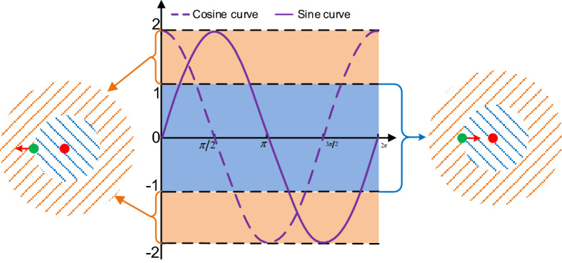
Diagram of SCA search mode.
The MSCA algorithm
In this section, a modified version of SCA is proposed to affronts the drawbacks of SCA exhibits optimization stagnation and slow convergence.
Modified position updating of SCA
In the original SCA, only the global optimal position is multiplied by a random factor, which only ensures that the population performs a local search to the current individual position, and ignores the existence of better potential solutions near the global optimal position.
In order to improve the convergence rate and ensure the search balance between the global optimal position and the current individual position, the update formula of SCA is reconstructed. When is less than 0.5, a search mode containing a sine function is used to find a potential better solution near the global optimal position. Otherwise, the cosine function formula is adopted to find a better solution near the current individual position. The modified position update as follows:
| 3 |
where represents the position vector of ith temporary individual at kth iteration. represents the position vector of ith individual at kth iteration. , and are random numbers for each position vector of ith temporary individual. represents the position vector of global best-known position at kth iteration.
Levy random walk mutation strategy
In SCA, only the global optimal individual is considered to guide the evolution direction of the population. When individual falls into a local optimal, it is difficult to jump out of the local unfavorable position only with the help of the global optimum position, which eventually leads to optimization stagnation.
Therefore, the personal best position11 and the Levy random walk37 is introduced into MSCA to make up for the shortcoming of cannot jump out of the local optimal. In order to take full advantage of the mutation operator, the global best position is used to form a difference vector with random individuals to act with the Levy random operator, and finally randomly superimposed on the current position or the personal best position to form a new individual. The Mantegna simulates Levy flight with different beta values as presented in Fig. 2. The expression of is defined as follows:
| 4 |
where represents the position vector of ith individual at (k + 1)th iteration. represents the position vector of personal best position of ith individual at kth iteration. and represent the index of randomly selected individuals in the temporary population, . represents the random vector in the interval [-1,1]. represents random vector with Levy distribution, is the tuning parameter.
Figure 2.

Mantegna simulates Levy flight with different beta values.
Execution steps of MSCA
The flowchart of the MSCA is shown in Fig. 3:
Figure 3.
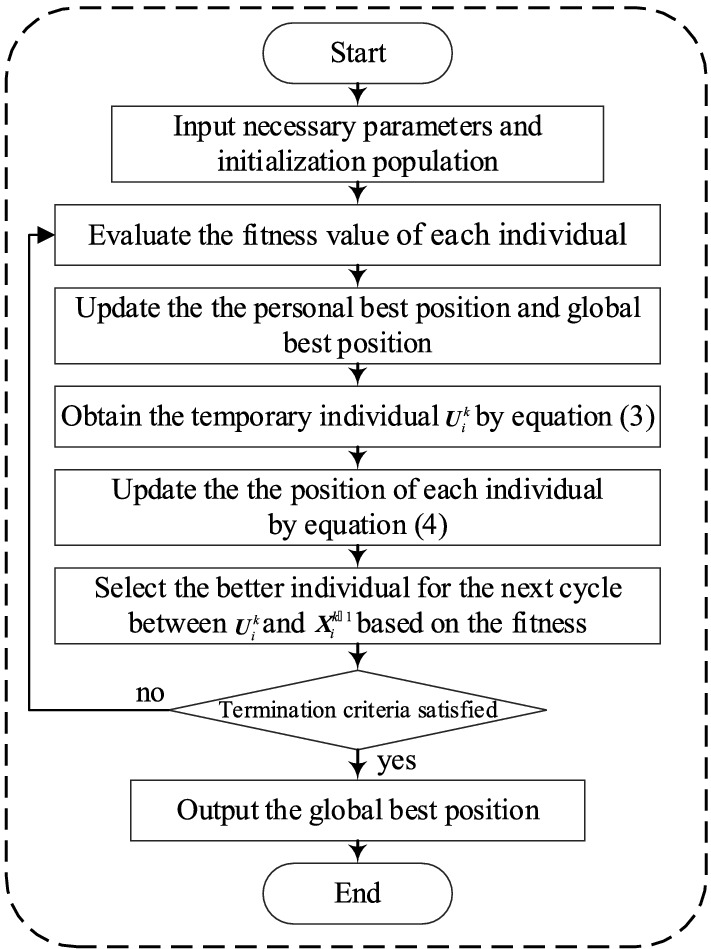
Flowchart of the MSCA method.
MSCA for numerical optimization problems
Compared with the SCA, MSCA has the advantages of better convergence speed and avoiding premature convergence because of the improved position update strategy and the Levy random walk mutation strategy. To further demonstrate the performance of MSCA, 24 classical benchmark problems38 and IEEE CEC2017 test suites39 are adopted to verify the effectiveness of proposed strategy.
Benchmark problem set I: classical benchmark problems
The first set of classical benchmark problems can be divided into unimodal (F1- F6), multimodal (F7-F13) and fixed-dimension multimodal (F14-F24). The unimodal was used to validate the convergence performance of the algorithm, the multimodal was used to test the ability of the method to avoid local stagnation, and the fixed-dimension multimodal was designed to examination the balance levels of the algorithm between exploration and exploitation. The 2D shape of the classical problem are listed in Fig. 4. The problems are listed in detail in Table 1. It is worth pointing out that fmin, range and n represent the theoretical optimal value, the upper and lower bounds and the dimension of the problem, respectively.
Figure 4.

A 2D shape of classical benchmark problems.
Table 1.
Details of 24 classical benchmark problems.
| Type | Equation | n | Range | fmin |
|---|---|---|---|---|
| Unimodal | 30 | [−100, 100] | 0 | |
| Unimodal | 30 | [−10, 10] | 0 | |
| Unimodal | 30 | [−100, 100] | 0 | |
| Unimodal | 30 | [−100, 100] | 0 | |
| Unimodal | 30 | [−30, 30] | 0 | |
| Unimodal | 30 | [−100, 100] | 0 | |
| Unimodal | 30 | [−1.28, 1.28] | 0 | |
| Multimodal | 30 | [−500, 500] | −12,567 | |
| Multimodal | 30 | [−5.12, 5.12] | 0 | |
| Multimodal | 30 | [−32, 32] | 0 | |
| Multimodal | 30 | [−600, 600] | 0 | |
| Multimodal | 30 | [−50, 50] | 0 | |
| Multimodal | 30 | [−50, 50] | 0 | |
| Fixed | 2 | [−65.536,65.536] | 1 | |
| Fixed | 4 | [−5, 5] | 0.0003075 | |
| Fixed | 2 | [−5, 5] | −1.0316285 | |
| Fixed | 2 | [−5,10] × [0,15] | 0.398 | |
| Fixed | 2 | [−2, 2] | 3 | |
| Fixed | 3 | [0,1] | −3.86 | |
| Fixed | 6 | [0,1] | −3.32 | |
| Fixed | 4 | [0,10] | −10.1532 | |
| Fixed | 4 | [0,10] | −10.4028 | |
| Fixed | 4 | [0,10] | −10.5363 | |
| Fixed | 2 | [−5, 5] | 0 |
Parameter settings
For fair comparison, seven existing persuasive algorithms are introduced to compare with MSCA, including GA40, PSO11, GSA8, JAYA41, ALO42, MVO43, GWO44, WOA4, SSA45, HGSO12, AOA46 and SCA2. the population size was set to 50, and the maximum iterations was set to 500 in the selected algorithm. For avoid the influence of randomness, each algorithm was independently repeated for 20 times. The default parameter value settings of all the algorithms are listed in Table 2.
Table 2.
The default parameters of selected algorithm.
| Algorithm | Detailed parameter | Value |
|---|---|---|
| GA | Mutation probability | 0.05 |
| Crossover probability | 0.6 | |
| PSO | Cognitive coefficient(C1) | 2.0 |
| Cognitive coefficient(C2) | 2.0 | |
| Weight (wmax) | 0.8 | |
| Weight (wmin) | 0.3 | |
| GSA | Attenuation factor a | 20 |
| Initial gravitational constant G0 | 100 | |
| MVO | Minimum of Wormhole Existence Probability | 0.2 |
| Maximum of Wormhole Existence Probability | 1.0 | |
| GWO | Constant a | 2.0 |
| WOA | Constant a | 2.0 |
| SSA | Coefficient c1 | |
| HGSO | Cluster number | 5 |
| AOA | Control parameter | 0.5 |
| Control parameter | 5 | |
| SCA | Constant a | 2.0 |
| MSCA | Constant a | 2.0 |
| Tuning parameter β | 1.5 |
Experimental results analysis
To obey the univariate principle, all algorithms are run independently in the same environment. The comparison results of selected algorithms for 24 benchmark problems are given in Table 3, including the mean and standard deviation (STD). The results of the Wilcoxon ranksum and signed-rank test at 5% level significance level are reported in Tables 4 and 5, respectively. It should be pointed out that in Table 5 , if the result of MSCA is better than the competitive algorithms, that the MSCA is recorded as win, if equal, recorded as tie, otherwise recorded as lose.
Table 3.
Comparison results of selected algorithms for classical benchmark problem.
| Function | Item | GA | PSO | GSA | JAYA | ALO | MVO | GWO | WOA | SSA | HGSO | AOA | SCA | MSCA |
|---|---|---|---|---|---|---|---|---|---|---|---|---|---|---|
| F1 | Mean | 1.45E + 03 | 8.84E-04 | 4.85E-12 | 3.98E + 01 | 1.43E-04 | 8.62E-01 | 1.93E-19 | 1.91E-69 | 2.85E-05 | 3.02E-17 | 3.51E-23 | 4.72E + 00 | 1.13E-75 |
| STD | 2.51E + 02 | 9.82E-04 | 6.97E-12 | 9.40E + 00 | 7.88E-05 | 2.07E-01 | 2.63E-19 | 7.12E-69 | 5.78E-05 | 1.14E-16 | 1.57E-22 | 8.71E + 00 | 6.21E-75 | |
| F2 | Mean | 1.28E + 01 | 5.00E + 00 | 7.37E-02 | 6.14E + 00 | 4.80E + 01 | 1.12E + 01 | 4.98E-12 | 8.59E-52 | 3.25E + 00 | 1.58E-15 | 3.26E-115 | 1.38E-02 | 6.76E-47 |
| STD | 1.71E + 00 | 6.82E + 00 | 2.64E-01 | 2.54E + 00 | 4.86E + 01 | 3.22E + 01 | 2.95E-12 | 3.72E-51 | 1.91E + 00 | 5.42E-15 | 1.01E-114 | 2.05E-02 | 1.94E-46 | |
| F3 | Mean | 2.07E + 04 | 5.90E + 03 | 7.04E + 02 | 3.85E + 04 | 2.35E + 03 | 7.84E + 01 | 5.07E-03 | 5.96E + 04 | 2.25E + 03 | 2.04E + 02 | 5.01E-03 | 6.92E + 03 | 8.51E + 00 |
| STD | 4.07E + 03 | 4.76E + 03 | 2.22E + 02 | 5.66E + 03 | 1.13E + 03 | 3.74E + 01 | 1.38E-02 | 1.91E + 04 | 7.83E + 02 | 3.76E + 02 | 1.12E-02 | 4.67E + 03 | 1.48E + 01 | |
| F4 | Mean | 2.26E + 01 | 7.77E + 00 | 4.03E + 00 | 2.74E + 01 | 1.75E + 01 | 1.47E + 00 | 1.92E-04 | 4.51E + 01 | 1.54E + 01 | 9.38E-02 | 3.51E-02 | 2.46E + 01 | 2.18E-32 |
| STD | 9.68E-01 | 1.77E + 00 | 1.14E + 00 | 5.56E + 00 | 5.31E + 00 | 6.18E-01 | 1.64E-04 | 2.87E + 01 | 5.75E + 00 | 1.94E-01 | 1.31E-02 | 9.57E + 00 | 1.19E-31 | |
| F5 | Mean | 2.56E + 05 | 3.85E + 03 | 8.91E + 01 | 3.88E + 03 | 2.53E + 02 | 3.62E + 02 | 2.79E + 01 | 2.85E + 01 | 4.50E + 02 | 2.82E + 01 | 2.85E + 01 | 1.61E + 04 | 2.55E + 01 |
| STD | 6.47E + 04 | 1.63E + 04 | 6.94E + 01 | 2.18E + 03 | 3.73E + 02 | 5.68E + 02 | 7.92E-01 | 3.41E-01 | 7.22E + 02 | 2.86E-01 | 2.40E-01 | 4.24E + 04 | 1.66E-01 | |
| F6 | Mean | 1.41E + 03 | 1.03E-03 | 6.09E-12 | 6.79E + 01 | 1.04E-04 | 8.26E-01 | 1.95E + 00 | 1.09E + 00 | 1.74E-05 | 3.40E + 00 | 3.84E + 00 | 8.48E + 00 | 8.46E-04 |
| STD | 2.46E + 02 | 1.10E-03 | 1.05E-11 | 2.22E + 01 | 5.34E-05 | 2.07E-01 | 6.30E-01 | 3.43E-01 | 2.26E-05 | 3.39E-01 | 2.60E-01 | 5.47E + 00 | 1.99E-03 | |
| F7 | Mean | 6.54E-01 | 1.04E + 00 | 5.55E-01 | 7.09E-01 | 5.72E-01 | 5.25E-01 | 3.67E-01 | 5.05E-01 | 6.95E-01 | 5.13E-01 | 4.54E-01 | 6.49E-01 | 4.52E-01 |
| STD | 3.14E-01 | 2.13E + 00 | 2.95E-01 | 2.85E-01 | 2.67E-01 | 2.74E-01 | 3.19E-01 | 2.21E-01 | 3.47E-01 | 2.84E-01 | 2.33E-01 | 2.57E-01 | 2.98E-01 | |
| F8 | Mean | -1.13E + 04 | -9.78E + 03 | -2.87E + 03 | -5.19E + 03 | -5.78E + 03 | -8.13E + 03 | -5.45E + 03 | -9.38E + 03 | -7.23E + 03 | -4.07E + 03 | -3.03E + 38 | -3.90E + 03 | -1.24E + 04 |
| STD | 2.02E + 02 | 6.03E + 02 | 4.19E + 02 | 5.98E + 02 | 8.90E + 02 | 7.61E + 02 | 8.05E + 02 | 1.77E + 03 | 8.03E + 02 | 5.81E + 02 | 1.35E + 39 | 2.99E + 02 | 6.26E + 02 | |
| F9 | Mean | 5.55E + 01 | 5.72E + 01 | 1.87E + 01 | 2.56E + 02 | 8.34E + 01 | 1.12E + 02 | 1.74E + 01 | 0.00E + 00 | 5.16E + 01 | 8.27E + 00 | 0.00E + 00 | 3.90E + 01 | 0.00E + 00 |
| STD | 6.38E + 00 | 1.81E + 01 | 4.11E + 00 | 2.00E + 01 | 2.03E + 01 | 3.14E + 01 | 5.25E + 00 | 0.00E + 00 | 1.43E + 01 | 2.69E + 01 | 0.00E + 00 | 3.87E + 01 | 0.00E + 00 | |
| F10 | Mean | 8.93E + 00 | 2.44E-01 | 9.00E-07 | 7.70E + 00 | 2.38E + 00 | 1.51E + 00 | 9.54E-11 | 4.09E-15 | 3.57E + 00 | 5.34E-10 | 0.00E + 00 | 1.38E + 01 | 0.00E + 00 |
| STD | 6.41E-01 | 4.66E-01 | 4.97E-07 | 6.11E + 00 | 8.25E-01 | 6.08E-01 | 6.30E-11 | 2.89E-15 | 1.18E + 00 | 1.82E-09 | 0.00E + 00 | 9.08E + 00 | 0.00E + 00 | |
| F11 | Mean | 1.40E + 01 | 1.72E-02 | 1.70E + 01 | 1.39E + 00 | 2.28E-02 | 7.58E-01 | 8.04E-03 | 0.00E + 00 | 4.53E-02 | 4.53E-12 | 3.47E-01 | 8.24E-01 | 0.00E + 00 |
| STD | 2.11E + 00 | 1.56E-02 | 3.87E + 00 | 1.11E-01 | 1.27E-02 | 9.93E-02 | 1.47E-02 | 0.00E + 00 | 2.88E-02 | 1.96E-11 | 1.82E-01 | 3.17E-01 | 0.00E + 00 | |
| F12 | Mean | 9.83E + 01 | 2.84E-01 | 1.18E + 00 | 1.93E + 01 | 1.15E + 01 | 1.35E + 00 | 1.55E-01 | 7.90E-02 | 8.39E + 00 | 5.33E-01 | 6.18E-01 | 4.07E + 03 | 2.42E-05 |
| STD | 1.85E + 02 | 3.95E-01 | 7.00E-01 | 9.80E + 00 | 4.75E + 00 | 1.10E + 00 | 1.32E-01 | 3.32E-02 | 3.15E + 00 | 1.50E-01 | 6.88E-02 | 2.21E + 04 | 5.04E-06 | |
| F13 | Mean | 7.12E + 04 | 5.61E-02 | 8.22E + 00 | 4.26E + 01 | 1.17E + 01 | 1.21E-01 | 1.40E + 00 | 1.28E + 00 | 2.86E + 01 | 2.48E + 00 | 2.67E + 00 | 3.81E + 04 | 3.78E-03 |
| STD | 3.87E + 04 | 7.19E-02 | 6.16E + 00 | 1.01E + 02 | 1.47E + 01 | 4.92E-02 | 2.78E-01 | 3.61E-01 | 1.40E + 01 | 1.77E-01 | 1.24E-01 | 1.91E + 05 | 1.87E-02 | |
| F14 | Mean | 9.98E-01 | 9.98E-01 | 4.03E + 00 | 9.98E-01 | 1.63E + 00 | 9.98E-01 | 5.93E + 00 | 3.20E + 00 | 1.25E + 00 | 1.38E + 00 | 8.37E + 00 | 1.40E + 00 | 9.98E-01 |
| STD | 9.96E-09 | 4.12E-17 | 2.98E + 00 | 2.73E-04 | 8.82E-01 | 5.00E-11 | 4.81E + 00 | 3.66E + 00 | 4.42E-01 | 4.71E-01 | 4.53E + 00 | 8.07E-01 | 1.43E-15 | |
| F15 | Mean | 1.05E-03 | 2.77E-03 | 6.28E-03 | 6.32E-04 | 3.50E-03 | 5.42E-03 | 4.41E-03 | 6.49E-04 | 4.81E-03 | 5.46E-04 | 1.88E-02 | 9.99E-04 | 6.13E-04 |
| STD | 4.01E-04 | 5.97E-03 | 3.33E-03 | 4.37E-04 | 6.73E-03 | 8.39E-03 | 8.19E-03 | 3.83E-04 | 8.04E-03 | 1.30E-04 | 3.39E-02 | 3.36E-04 | 4.11E-04 | |
| F16 | Mean | -1.03E + 00 | -1.03E + 00 | -1.03E + 00 | -1.03E + 00 | -1.03E + 00 | -1.03E + 00 | -1.03E + 00 | -1.03E + 00 | -1.03E + 00 | -1.03E + 00 | -1.03E + 00 | -1.03E + 00 | -1.03E + 00 |
| STD | 2.27E-05 | 6.71E-16 | 1.00E-15 | 3.05E-05 | 7.51E-14 | 5.14E-07 | 1.26E-08 | 6.85E-09 | 6.21E-14 | 1.80E-05 | 1.89E-07 | 3.75E-05 | 1.58E-13 | |
| F17 | Mean | 3.98E-01 | 3.98E-01 | 3.98E-01 | 3.99E-01 | 3.98E-01 | 3.98E-01 | 3.98E-01 | 3.98E-01 | 3.98E-01 | 3.99E-01 | 4.18E-01 | 4.00E-01 | 3.98E-01 |
| STD | 8.57E-05 | 0.00E + 00 | 8.97E-15 | 1.66E-03 | 3.89E-14 | 7.72E-07 | 2.13E-06 | 3.99E-04 | 6.10E-13 | 1.37E-03 | 1.27E-02 | 1.67E-03 | 7.78E-11 | |
| F18 | Mean | 3.00E + 00 | 3.00E + 00 | 3.00E + 00 | 3.00E + 00 | 3.00E + 00 | 3.00E + 00 | 3.00E + 00 | 3.00E + 00 | 3.00E + 00 | 3.00E + 00 | 2.17E + 01 | 3.00E + 00 | 3.00E + 00 |
| STD | 4.14E-04 | 1.24E-15 | 1.10E-13 | 7.97E-04 | 3.65E-13 | 4.09E-06 | 1.53E-04 | 3.99E-03 | 8.44E-13 | 3.75E-04 | 3.20E + 01 | 2.47E-05 | 7.71E-13 | |
| F19 | Mean | -3.86E + 00 | -3.86E + 00 | -3.70E + 00 | -3.86E + 00 | -3.86E + 00 | -3.86E + 00 | -3.86E + 00 | -3.83E + 00 | -3.86E + 00 | -3.86E + 00 | -3.85E + 00 | -3.86E + 00 | -3.86E + 00 |
| STD | 7.35E-06 | 2.65E-15 | 2.46E-01 | 2.71E-15 | 1.00E-13 | 2.19E-06 | 2.09E-03 | 5.36E-02 | 2.39E-02 | 3.36E-03 | 4.64E-03 | 3.40E-03 | 9.53E-10 | |
| F20 | Mean | -3.28E + 00 | -3.28E + 00 | -2.29E + 00 | -3.24E + 00 | -3.26E + 00 | -3.25E + 00 | -3.27E + 00 | -3.08E + 00 | -3.28E + 00 | -3.27E + 00 | -3.00E + 00 | -3.03E + 00 | -3.29E + 00 |
| STD | 5.69E-02 | 6.57E-02 | 7.37E-01 | 6.01E-02 | 6.06E-02 | 5.89E-02 | 8.36E-02 | 2.68E-01 | 8.77E-02 | 6.66E-02 | 1.06E-01 | 1.37E-01 | 5.11E-02 | |
| F21 | Mean | -6.95E + 00 | -8.48E + 00 | -4.98E + 00 | -7.22E + 00 | -5.94E + 00 | -6.87E + 00 | -9.53E + 00 | -7.52E + 00 | -9.40E + 00 | -8.09E + 00 | -4.40E + 00 | -2.56E + 00 | -9.30E + 00 |
| STD | 3.54E + 00 | 2.90E + 00 | 4.22E-01 | 2.46E + 00 | 2.75E + 00 | 3.04E + 00 | 1.97E + 00 | 2.54E + 00 | 1.85E + 00 | 1.99E + 00 | 1.74E + 00 | 1.94E + 00 | 1.93E + 00 | |
| F22 | Mean | -7.45E + 00 | -8.28E + 00 | -8.10E + 00 | -8.99E + 00 | -7.25E + 00 | -9.80E + 00 | -1.01E + 01 | -7.80E + 00 | -8.96E + 00 | -7.49E + 00 | -3.62E + 00 | -4.34E + 00 | -1.02E + 01 |
| STD | 3.49E + 00 | 3.12E + 00 | 2.68E + 00 | 2.15E + 00 | 3.08E + 00 | 1.88E + 00 | 1.19E + 00 | 2.81E + 00 | 2.60E + 00 | 2.41E + 00 | 1.66E + 00 | 1.62E + 00 | 9.70E-01 | |
| F23 | Mean | -7.39E + 00 | -9.61E + 00 | -9.11E + 00 | -8.96E + 00 | -8.08E + 00 | -9.73E + 00 | -9.72E + 00 | -7.09E + 00 | -1.05E + 01 | -8.09E + 00 | -3.85E + 00 | -4.70E + 00 | -9.82E + 00 |
| STD | 3.64E + 00 | 2.44E + 00 | 2.70E + 00 | 2.27E + 00 | 3.36E + 00 | 2.14E + 00 | 2.50E + 00 | 2.83E + 00 | 3.26E-10 | 2.29E + 00 | 1.91E + 00 | 1.23E + 00 | 1.87E + 00 | |
| F24 | Mean | 9.09E-05 | 8.77E-73 | 3.38E-16 | 6.39E-47 | 2.41E-13 | 1.90E-06 | 2.75E-148 | 8.74E-94 | 1.15E-13 | 1.07E-118 | 0.00E + 00 | 8.00E-78 | 2.31E-229 |
| STD | 1.13E-04 | 1.77E-72 | 6.02E-16 | 2.08E-46 | 2.21E-13 | 1.67E-06 | 1.21E-147 | 3.91E-93 | 1.12E-13 | 3.92E-118 | 0.00E + 00 | 2.99E-77 | 0.00E + 00 |
Significant values are in bold.
Table 4.
Wilcoxon ranksum test on classical benchmark functions at 5% level of significance.
| Function | GA vs MSCA | PSO vs MSCA | GSA vs MSCA | JAYA vs MSCA | ALO vs MSCA | MVO vs MSCA | GWO vs MSCA | WOA vs MSCA | SSA vs MSCA | HGSO vs MSCA | AOA vs MSCA | SCA vs MSCA |
|---|---|---|---|---|---|---|---|---|---|---|---|---|
| F1 | 6.80E-08 | 6.80E-08 | 6.80E-08 | 6.80E-08 | 6.80E-08 | 6.80E-08 | 6.80E-08 | 1.92E-07 | 6.80E-08 | 6.80E-08 | 6.80E-08 | 6.80E-08 |
| F2 | 6.80E-08 | 6.80E-08 | 6.80E-08 | 6.80E-08 | 6.80E-08 | 6.80E-08 | 6.80E-08 | 3.94E-07 | 6.80E-08 | 6.80E-08 | 6.80E-08 | 6.80E-08 |
| F3 | 6.80E-08 | 6.80E-08 | 6.80E-08 | 6.80E-08 | 6.80E-08 | 1.06E-07 | 3.29E-05 | 6.80E-08 | 6.80E-08 | 4.90E-01 | 2.69E-06 | 6.80E-08 |
| F4 | 6.80E-08 | 6.80E-08 | 6.80E-08 | 6.80E-08 | 6.80E-08 | 6.80E-08 | 6.80E-08 | 6.80E-08 | 6.80E-08 | 6.80E-08 | 6.80E-08 | 6.80E-08 |
| F5 | 6.80E-08 | 1.20E-06 | 6.80E-08 | 6.80E-08 | 1.20E-06 | 6.80E-08 | 6.80E-08 | 6.80E-08 | 6.80E-08 | 6.80E-08 | 6.80E-08 | 6.80E-08 |
| F6 | 6.80E-08 | 4.57E-01 | 6.80E-08 | 6.80E-08 | 6.80E-08 | 6.80E-08 | 6.80E-08 | 6.80E-08 | 6.80E-08 | 6.80E-08 | 6.80E-08 | 6.80E-08 |
| F7 | 6.80E-08 | 6.80E-08 | 6.80E-08 | 6.80E-08 | 6.80E-08 | 6.80E-08 | 1.16E-04 | 6.80E-08 | 6.80E-08 | 6.80E-08 | 3.94E-07 | 2.56E-07 |
| F8 | 1.20E-06 | 6.92E-07 | 6.80E-08 | 6.80E-08 | 6.46E-08 | 1.23E-07 | 6.80E-08 | 1.80E-06 | 6.80E-08 | 6.80E-08 | 1.60E-05 | 6.80E-08 |
| F9 | 8.01E-09 | 8.01E-09 | 8.01E-09 | 8.01E-09 | 8.01E-09 | 8.01E-09 | 8.01E-09 | N/A | 8.01E-09 | 6.68E-05 | N/A | 8.01E-09 |
| F10 | 8.01E-09 | 8.01E-09 | 8.01E-09 | 8.01E-09 | 8.01E-09 | 8.01E-09 | 8.01E-09 | 2.71E-06 | 8.01E-09 | 7.86E-09 | N/A | 8.01E-09 |
| F11 | 8.01E-09 | 8.01E-09 | 8.01E-09 | 8.01E-09 | 8.01E-09 | 8.01E-09 | 3.37E-07 | N/A | 8.01E-09 | 1.98E-02 | 8.01E-09 | 8.01E-09 |
| F12 | 6.80E-08 | 6.80E-08 | 6.80E-08 | 6.80E-08 | 6.80E-08 | 6.80E-08 | 6.80E-08 | 6.80E-08 | 6.80E-08 | 6.80E-08 | 6.80E-08 | 6.80E-08 |
| F13 | 6.80E-08 | 6.92E-07 | 7.90E-08 | 6.80E-08 | 9.17E-08 | 2.56E-07 | 6.80E-08 | 6.80E-08 | 6.80E-08 | 6.80E-08 | 6.80E-08 | 6.80E-08 |
| F14 | 4.67E-08 | 4.91E-09 | 8.85E-07 | 4.67E-08 | 4.41E-01 | 4.67E-08 | 4.61E-08 | 4.67E-08 | 5.88E-01 | 4.67E-08 | 4.67E-08 | 4.67E-08 |
| F15 | 3.15E-02 | 9.07E-02 | 6.80E-08 | 1.64E-01 | 3.15E-02 | 6.04E-03 | 9.25E-01 | 3.51E-01 | 9.79E-03 | 3.94E-01 | 9.21E-04 | 9.79E-03 |
| F16 | 6.66E-08 | 7.80E-09 | 7.80E-09 | 6.66E-08 | 1.14E-02 | 6.66E-08 | 6.66E-08 | 6.66E-08 | 2.48E-03 | 6.66E-08 | 6.66E-08 | 6.66E-08 |
| F17 | 6.80E-08 | 8.01E-09 | 4.63E-08 | 1.71E-01 | 8.50E-07 | 6.80E-08 | 6.80E-08 | 6.80E-08 | 1.41E-05 | 6.80E-08 | 6.80E-08 | 6.80E-08 |
| F18 | 6.76E-08 | 7.95E-09 | 2.26E-04 | 6.76E-08 | 4.02E-01 | 6.76E-08 | 6.76E-08 | 6.76E-08 | 8.29E-01 | 6.76E-08 | 8.47E-07 | 6.76E-08 |
| F19 | 6.80E-08 | 8.01E-09 | 6.80E-08 | 8.01E-09 | 6.46E-08 | 6.80E-08 | 6.80E-08 | 6.80E-08 | 9.13E-07 | 6.80E-08 | 6.80E-08 | 6.80E-08 |
| F20 | 6.61E-05 | 2.34E-01 | 1.61E-04 | 8.37E-01 | 9.25E-01 | 5.87E-06 | 1.16E-04 | 2.06E-06 | 7.11E-03 | 3.75E-04 | 6.80E-08 | 2.22E-07 |
| F21 | 2.60E-05 | 2.81E-03 | 7.94E-04 | 1.78E-03 | 9.79E-03 | 2.60E-05 | 8.36E-04 | 1.60E-05 | 4.17E-05 | 2.47E-04 | 5.87E-06 | 1.23E-07 |
| F22 | 6.92E-07 | 2.25E-02 | 4.39E-01 | 6.74E-01 | 4.90E-01 | 1.05E-06 | 1.05E-06 | 3.42E-07 | 5.12E-03 | 4.54E-07 | 1.23E-07 | 1.92E-07 |
| F23 | 1.58E-06 | 6.80E-05 | 8.00E-05 | 3.09E-01 | 7.64E-02 | 7.58E-06 | 9.75E-06 | 6.92E-07 | 6.80E-08 | 4.54E-06 | 2.22E-07 | 1.66E-07 |
| F24 | 6.80E-08 | 6.80E-08 | 6.80E-08 | 6.80E-08 | 6.80E-08 | 6.80E-08 | 6.80E-08 | 6.80E-08 | 6.80E-08 | 6.80E-08 | 8.01E-09 | 6.80E-08 |
Significant values are in bold.
Table 5.
Wilcoxon signed-rank test on classical benchmark functions at 5% level of significance.
| Item | Win | Tie | Lose | R+ | R- | p-value | Decision |
|---|---|---|---|---|---|---|---|
| GA vs MSCA | 24 | 0 | 0 | 300 | 0 | 1.82E-05 | + |
| PSO vs MSCA | 19 | 0 | 5 | 280 | 20 | 2.04E-04 | + |
| GSA vs MSCA | 20 | 0 | 4 | 283 | 17 | 1.45E-04 | + |
| JAYA vs MSCA | 23 | 0 | 1 | 298 | 2 | 2.35E-05 | + |
| ALO vs MSCA | 19 | 0 | 5 | 281 | 19 | 1.82E-04 | + |
| MVO vs MSCA | 24 | 0 | 0 | 300 | 0 | 1.82E-05 | + |
| GWO vs MSCA | 21 | 0 | 3 | 248 | 52 | 5.11E-03 | + |
| WOA vs MSCA | 21 | 2 | 1 | 293.5 | 6.5 | 6.08E-05 | + |
| SSA vs MSCA | 19 | 0 | 5 | 263 | 37 | 1.24E-03 | + |
| AOA vs MSCA | 18 | 2 | 4 | 245.5 | 54.5 | 8.15E-03 | + |
| SCA vs MSCA | 24 | 0 | 0 | 300 | 0 | 1.82E-05 | + |
From Table 3, MSCA outperforms GA, MVO and SCA on the mean of all benchmark problems, and the standard deviation of MSCA is smaller than SCA. Furthermore, MSCA wins most problems compared to PSO, GSA, JAYA and ALO.
In Table 4, The p-value of the vast majority of rank sum tests are less than 5%, which illustrates the variability in the overall distribution of target values for the proposed and control methods. At the same time, MSCA achieved p-values of less than 5% in all sign-rank comparisons in Table 5, indicating that the results obtained by MSCA are statistically significant. Overall, MSCA can balance the process between exploration and exploitation.
Robustness and convergence analysis
For validate the robustness and convergence performance of MSCA in classical benchmark problems, the box-plot of all results and convergence curve of best result for JAYA, ALO, MVO, SCA and MSCA are plotted in Figs. 5 and 6.respectively.
Figure 5.

The box-plot of different algorithms on classical benchmark problems.
Figure 6.

The convergence curve on classical benchmark problems.
Box-plot revealed the distribution of results obtained by each method. It can be seen from Fig. 5 that JAYA, ALO, MVO and SCA show different degrees of dispersion in different benchmark problems, while MCSA get more stable and better distribution. And it can be seen from the convergence curve in Fig. 6 that MSCA has a faster convergence rate than other algorithms. Hence, the modified SCA position update formula combined with Levy random walk mutation strategy can get more accurate results.
Benchmark problem set II: CEC2017 test suites
In this section, IEEE CEC2017 test suites are adopted to prove the performance of MSCA, which are mainly divided into four groups: (a) Unimodal, (b) Multimodal, (c) Hybrid and (d) Composition. The definition of the CEC2017 benchmark problems is shown in Table 6. Unlike classical benchmark function problems, this problem involves matrix rotation and global optimum shifted operations.
Table 6.
The definition of CEC2017 test suites.
| Type | Function | Name | n | Range | fmin |
|---|---|---|---|---|---|
| Unimodal | F1: | Shifted and Rotated Bent Cigar Function | 10 | [−100, 100] | 100 |
| Unimodal | F2: | Shifted and Rotated Sum of Different Power Function | 10 | [−100, 100] | 200 |
| Unimodal | F3: | Shifted and Rotated Zakharov Function | 10 | [−100, 100] | 300 |
| Multimodal | F4: | Shifted and Rotated Rosenbrock’s Function | 10 | [−100, 100] | 400 |
| Multimodal | F5: | Shifted and Rotated Rastrigin’s Function | 10 | [−100, 100] | 500 |
| Multimodal | F6: | Shifted and Rotated Expanded Scaffer’s F6 Function | 10 | [−100, 100] | 600 |
| Multimodal | F7: | Shifted and Rotated Lunacek Bi_Rastrigin Function | 10 | [−100, 100] | 700 |
| Multimodal | F8: | Shifted and Rotated Non−Continuous Rastrigin’s Function | 10 | [−100, 100] | 800 |
| Multimodal | F9: | Shifted and Rotated Levy Function | 10 | [−100, 100] | 900 |
| Multimodal | F10: | Shifted and Rotated Schwefel’s Function | 10 | [−100, 100] | 1000 |
| Hybrid | F11: | Hybrid Function 1 (N = 3) | 10 | [−100, 100] | 1100 |
| Hybrid | F12: | Hybrid Function 2 (N = 3) | 10 | [−100, 100] | 1200 |
| Hybrid | F13: | Hybrid Function 3 (N = 3) | 10 | [−100, 100] | 1300 |
| Hybrid | F14: | Hybrid Function 4 (N = 4) | 10 | [−100, 100] | 1400 |
| Hybrid | F15: | Hybrid Function 5 (N = 4) | 10 | [−100, 100] | 1500 |
| Hybrid | F16: | Hybrid Function 6 (N = 4) | 10 | [−100, 100] | 1600 |
| Hybrid | F17: | Hybrid Function 6 (N = 5) | 10 | [−100, 100] | 1700 |
| Hybrid | F18: | Hybrid Function 6 (N = 5) | 10 | [−100, 100] | 1800 |
| Hybrid | F19: | Hybrid Function 6 (N = 5) | 10 | [−100, 100] | 1900 |
| Hybrid | F20: | Hybrid Function 6 (N = 6) | 10 | [−100, 100] | 2000 |
| Composition | F21: | Composition Function 1 (N = 3) | 10 | [−100, 100] | 2100 |
| Composition | F22: | Composition Function 2 (N = 3) | 10 | [−100, 100] | 2200 |
| Composition | F23: | Composition Function 3 (N = 4) | 10 | [−100, 100] | 2300 |
| Composition | F24: | Composition Function 4 (N = 4) | 10 | [−100, 100] | 2400 |
| Composition | F25: | Composition Function 5 (N = 5) | 10 | [−100, 100] | 2500 |
| Composition | F26: | Composition Function 6 (N = 5) | 10 | [−100, 100] | 2600 |
| Composition | F27: | Composition Function 7 (N = 6) | 10 | [−100, 100] | 2700 |
| Composition | F28: | Composition Function 8 (N = 6) | 10 | [−100, 100] | 2800 |
| Composition | F29: | Composition Function 9 (N = 3) | 10 | [−100, 100] | 2900 |
| Composition | F30: | Composition Function 10 (N = 3) | 10 | [−100, 100] | 3000 |
Experimental results analysis
The statistical results for CEC2017 are illustrated in Table 7. From the table, it can be concluded that MSCA outperforms the other popular methods in most of the CEC2017 benchmark problems. In addition, from the results of the Wilcoxon ranksum and signed-rank test in Tables 8 and 9, it can be concluded that the proposed method is effective in improving the search efficiency of SCA and provides better results than other methods. In conclusion, MSCA is a quite competitive algorithm.
Table 7.
Statistic result of the algorithms on CEC2017 test suit with 10 dimensions.
| Function | Item | GA | PSO | GSA | JAYA | ALO | MVO | GWO | WOA | SSA | HGSO | AOA | SCA | MSCA |
|---|---|---|---|---|---|---|---|---|---|---|---|---|---|---|
| F1 | Mean | 1.12E + 07 | 9.35E + 06 | 3.28E + 02 | 3.81E + 08 | 1.84E + 03 | 1.69E + 04 | 1.78E + 08 | 4.47E + 08 | 2.13E + 03 | 4.40E + 08 | 1.02E + 10 | 8.37E + 08 | 1.55E + 05 |
| STD | 5.63E + 06 | 2.42E + 07 | 4.24E + 02 | 1.49E + 08 | 1.89E + 03 | 5.93E + 03 | 2.06E + 08 | 2.87E + 08 | 2.22E + 03 | 4.52E + 08 | 4.29E + 09 | 2.45E + 08 | 8.44E + 04 | |
| F2 | Mean | 6.44E + 06 | 1.04E + 09 | 4.60E + 10 | 4.31E + 07 | 1.43E + 03 | 7.26E + 02 | 5.45E + 09 | 5.69E + 09 | 2.04E + 05 | 6.10E + 08 | 8.30E + 14 | 1.19E + 09 | 1.74E + 05 |
| STD | 1.22E + 07 | 5.58E + 09 | 7.19E + 10 | 4.05E + 07 | 2.69E + 03 | 1.03E + 03 | 9.60E + 09 | 1.58E + 10 | 3.55E + 05 | 1.86E + 09 | 1.39E + 15 | 2.48E + 09 | 3.18E + 05 | |
| F3 | Mean | 3.79E + 03 | 3.00E + 02 | 1.58E + 04 | 8.46E + 03 | 3.00E + 02 | 3.00E + 02 | 5.17E + 03 | 1.24E + 04 | 3.45E + 02 | 3.28E + 03 | 1.50E + 04 | 2.14E + 03 | 3.79E + 02 |
| STD | 1.47E + 03 | 3.60E-03 | 3.32E + 03 | 2.05E + 03 | 1.68E-01 | 7.99E-02 | 2.85E + 03 | 8.10E + 03 | 1.36E + 02 | 1.30E + 03 | 4.11E + 03 | 1.35E + 03 | 5.77E + 01 | |
| F4 | Mean | 4.07E + 02 | 4.24E + 02 | 4.25E + 02 | 4.10E + 02 | 4.11E + 02 | 4.05E + 02 | 4.29E + 02 | 4.80E + 02 | 4.06E + 02 | 4.35E + 02 | 1.13E + 03 | 4.54E + 02 | 4.07E + 02 |
| STD | 9.05E-01 | 3.94E + 01 | 1.79E + 01 | 6.11E-01 | 1.76E + 01 | 1.47E + 00 | 2.82E + 01 | 5.93E + 01 | 2.20E + 00 | 1.82E + 01 | 4.70E + 02 | 2.06E + 01 | 5.94E-01 | |
| F5 | Mean | 5.68E + 02 | 1.08E + 03 | 6.13E + 02 | 1.13E + 03 | 5.24E + 02 | 5.29E + 02 | 5.25E + 02 | 5.69E + 02 | 5.30E + 02 | 5.44E + 02 | 5.71E + 02 | 1.95E + 03 | 5.34E + 02 |
| STD | 1.42E + 01 | 8.77E + 02 | 1.73E + 02 | 2.05E + 02 | 8.60E + 00 | 1.19E + 01 | 1.37E + 01 | 2.17E + 01 | 1.32E + 01 | 8.66E + 00 | 1.89E + 01 | 4.93E + 02 | 6.38E + 00 | |
| F6 | Mean | 6.00E + 02 | 6.00E + 02 | 6.00E + 02 | 6.00E + 02 | 6.00E + 02 | 6.00E + 02 | 6.05E + 02 | 6.45E + 02 | 6.21E + 02 | 6.14E + 02 | 6.42E + 02 | 6.00E + 02 | 6.00E + 02 |
| STD | 3.47E-03 | 4.87E-03 | 3.24E-02 | 1.10E-02 | 2.79E-02 | 1.13E-02 | 3.49E + 00 | 1.33E + 01 | 1.05E + 01 | 7.71E + 00 | 5.27E + 00 | 1.58E-02 | 1.51E-04 | |
| F7 | Mean | 7.37E + 02 | 7.24E + 02 | 7.24E + 02 | 7.63E + 02 | 7.41E + 02 | 7.29E + 02 | 7.41E + 02 | 7.94E + 02 | 7.39E + 02 | 7.65E + 02 | 7.93E + 02 | 7.81E + 02 | 7.29E + 02 |
| STD | 5.81E + 00 | 5.27E + 00 | 5.67E + 00 | 8.03E + 00 | 1.41E + 01 | 9.68E + 00 | 1.57E + 01 | 2.01E + 01 | 1.16E + 01 | 1.17E + 01 | 1.27E + 01 | 1.01E + 01 | 4.03E + 00 | |
| F8 | Mean | 8.16E + 02 | 8.13E + 02 | 8.23E + 02 | 8.47E + 02 | 8.21E + 02 | 8.19E + 02 | 8.20E + 02 | 8.47E + 02 | 8.30E + 02 | 8.40E + 02 | 8.45E + 02 | 8.45E + 02 | 8.09E + 02 |
| STD | 3.26E + 00 | 5.14E + 00 | 6.23E + 00 | 6.18E + 00 | 1.03E + 01 | 9.59E + 00 | 7.64E + 00 | 1.84E + 01 | 9.80E + 00 | 7.50E + 00 | 1.25E + 01 | 7.41E + 00 | 2.69E + 00 | |
| F9 | Mean | 9.00E + 02 | 9.00E + 02 | 9.00E + 02 | 9.00E + 02 | 9.00E + 02 | 9.00E + 02 | 9.46E + 02 | 1.81E + 03 | 1.03E + 03 | 9.79E + 02 | 1.39E + 03 | 9.00E + 02 | 9.00E + 02 |
| STD | 1.93E-02 | 1.45E-01 | 5.83E-01 | 1.00E-01 | 3.14E-01 | 6.88E-01 | 6.89E + 01 | 6.45E + 02 | 1.50E + 02 | 5.27E + 01 | 2.13E + 02 | 1.44E-01 | 5.26E-05 | |
| F10 | Mean | 1.49E + 03 | 1.52E + 03 | 2.90E + 03 | 2.25E + 03 | 2.00E + 03 | 1.70E + 03 | 1.88E + 03 | 2.32E + 03 | 1.96E + 03 | 2.59E + 03 | 2.43E + 03 | 2.40E + 03 | 1.29E + 03 |
| STD | 1.51E + 02 | 2.15E + 02 | 2.40E + 02 | 2.26E + 02 | 3.94E + 02 | 2.66E + 02 | 4.13E + 02 | 3.71E + 02 | 3.27E + 02 | 2.07E + 02 | 2.66E + 02 | 2.01E + 02 | 1.36E + 02 | |
| F11 | Mean | 1.27E + 03 | 1.17E + 03 | 1.17E + 04 | 2.61E + 03 | 1.17E + 03 | 1.14E + 03 | 1.18E + 03 | 1.36E + 03 | 1.17E + 03 | 1.18E + 03 | 5.60E + 03 | 2.68E + 03 | 1.13E + 03 |
| STD | 8.15E + 01 | 3.13E + 02 | 2.65E + 03 | 4.85E + 02 | 6.92E + 01 | 7.33E + 01 | 9.02E + 01 | 2.60E + 02 | 4.89E + 01 | 2.79E + 01 | 6.71E + 03 | 1.14E + 03 | 2.14E + 01 | |
| F12 | Mean | 6.64E + 05 | 1.11E + 06 | 1.50E + 06 | 9.96E + 06 | 1.97E + 06 | 1.27E + 06 | 8.08E + 05 | 4.53E + 06 | 3.27E + 06 | 7.92E + 06 | 3.71E + 08 | 1.72E + 07 | 1.84E + 05 |
| STD | 5.07E + 05 | 2.83E + 06 | 8.49E + 05 | 9.25E + 06 | 2.11E + 06 | 1.13E + 06 | 8.92E + 05 | 5.44E + 06 | 4.58E + 06 | 6.79E + 06 | 3.07E + 08 | 1.68E + 07 | 3.41E + 05 | |
| F13 | Mean | 1.22E + 04 | 8.39E + 03 | 1.13E + 04 | 1.85E + 04 | 1.51E + 04 | 1.30E + 04 | 1.35E + 04 | 1.77E + 04 | 1.66E + 04 | 3.16E + 04 | 2.51E + 07 | 4.33E + 04 | 3.97E + 03 |
| STD | 8.41E + 03 | 8.48E + 03 | 2.18E + 03 | 1.63E + 04 | 1.30E + 04 | 1.07E + 04 | 9.55E + 03 | 1.91E + 04 | 1.10E + 04 | 2.71E + 04 | 6.38E + 07 | 2.47E + 04 | 4.03E + 03 | |
| F14 | Mean | 2.34E + 03 | 2.08E + 03 | 1.42E + 04 | 4.40E + 03 | 1.24E + 04 | 1.98E + 03 | 5.24E + 03 | 2.97E + 03 | 4.13E + 03 | 2.77E + 03 | 7.80E + 03 | 6.49E + 03 | 1.46E + 03 |
| STD | 1.03E + 03 | 1.03E + 03 | 2.86E + 03 | 1.70E + 03 | 6.85E + 03 | 8.71E + 02 | 2.40E + 03 | 1.75E + 03 | 4.15E + 03 | 1.35E + 03 | 7.29E + 03 | 2.24E + 03 | 1.46E + 01 | |
| F15 | Mean | 2.95E + 03 | 4.63E + 03 | 2.87E + 04 | 1.02E + 04 | 3.08E + 04 | 3.01E + 03 | 9.88E + 03 | 1.00E + 04 | 9.93E + 03 | 4.50E + 03 | 1.61E + 04 | 8.43E + 03 | 1.59E + 03 |
| STD | 1.37E + 03 | 6.30E + 03 | 5.87E + 03 | 6.34E + 03 | 1.65E + 04 | 2.27E + 03 | 6.75E + 03 | 6.62E + 03 | 7.74E + 03 | 2.42E + 03 | 7.72E + 03 | 3.37E + 03 | 1.32E + 02 | |
| F16 | Mean | 1.66E + 03 | 1.74E + 03 | 2.25E + 03 | 1.73E + 03 | 1.90E + 03 | 1.75E + 03 | 1.79E + 03 | 2.05E + 03 | 1.82E + 03 | 1.80E + 03 | 2.13E + 03 | 1.80E + 03 | 1.62E + 03 |
| STD | 6.33E + 01 | 1.34E + 02 | 1.05E + 02 | 4.75E + 01 | 1.85E + 02 | 1.25E + 02 | 1.29E + 02 | 2.08E + 02 | 1.62E + 02 | 8.73E + 01 | 1.81E + 02 | 9.61E + 01 | 3.22E + 01 | |
| F17 | Mean | 1.74E + 03 | 1.78E + 03 | 1.88E + 03 | 1.93E + 03 | 1.83E + 03 | 1.82E + 03 | 1.78E + 03 | 1.84E + 03 | 1.78E + 03 | 1.78E + 03 | 1.89E + 03 | 1.90E + 03 | 1.73E + 03 |
| STD | 1.93E + 01 | 6.23E + 01 | 1.51E + 02 | 5.63E + 01 | 1.03E + 02 | 7.46E + 01 | 3.27E + 01 | 6.59E + 01 | 2.39E + 01 | 1.25E + 01 | 8.68E + 01 | 7.55E + 01 | 8.08E + 00 | |
| F18 | Mean | 1.40E + 04 | 3.36E + 04 | 2.44E + 04 | 1.01E + 05 | 4.40E + 04 | 2.07E + 04 | 2.14E + 04 | 1.90E + 04 | 2.13E + 04 | 2.44E + 05 | 2.54E + 08 | 2.29E + 05 | 8.86E + 03 |
| STD | 1.03E + 04 | 2.16E + 04 | 6.49E + 03 | 5.95E + 04 | 2.99E + 04 | 1.44E + 04 | 1.73E + 04 | 1.32E + 04 | 1.44E + 04 | 3.60E + 05 | 4.88E + 08 | 2.43E + 05 | 6.47E + 03 | |
| F19 | Mean | 5.01E + 03 | 1.36E + 04 | 6.44E + 05 | 1.10E + 04 | 2.58E + 04 | 2.47E + 03 | 2.94E + 04 | 4.73E + 05 | 7.15E + 03 | 6.58E + 03 | 4.99E + 06 | 1.24E + 04 | 1.97E + 03 |
| STD | 3.61E + 03 | 1.65E + 04 | 5.57E + 05 | 1.01E + 04 | 1.77E + 04 | 8.24E + 02 | 6.97E + 04 | 8.96E + 05 | 6.74E + 03 | 4.53E + 03 | 2.15E + 07 | 8.02E + 03 | 1.06E + 02 | |
| F20 | Mean | 2.03E + 03 | 2.08E + 03 | 2.39E + 03 | 2.27E + 03 | 2.20E + 03 | 2.16E + 03 | 2.14E + 03 | 2.24E + 03 | 2.13E + 03 | 2.11E + 03 | 2.16E + 03 | 2.29E + 03 | 2.02E + 03 |
| STD | 8.67E + 00 | 8.39E + 01 | 1.34E + 02 | 6.44E + 01 | 1.02E + 02 | 8.87E + 01 | 7.87E + 01 | 8.93E + 01 | 6.71E + 01 | 3.51E + 01 | 6.19E + 01 | 6.56E + 01 | 2.21E + 01 | |
| F21 | Mean | 2.27E + 03 | 2.56E + 03 | 2.32E + 03 | 2.67E + 03 | 2.21E + 03 | 2.25E + 03 | 2.32E + 03 | 2.34E + 03 | 2.28E + 03 | 2.24E + 03 | 2.36E + 03 | 2.62E + 03 | 2.20E + 03 |
| STD | 5.06E + 01 | 2.47E + 02 | 9.78E + 01 | 6.89E + 01 | 3.19E + 01 | 6.49E + 01 | 9.00E + 00 | 4.81E + 01 | 5.97E + 01 | 2.01E + 01 | 3.66E + 01 | 2.15E + 02 | 5.03E-01 | |
| F22 | Mean | 2.31E + 03 | 2.32E + 03 | 2.39E + 03 | 2.33E + 03 | 2.30E + 03 | 2.37E + 03 | 2.37E + 03 | 2.63E + 03 | 2.30E + 03 | 2.34E + 03 | 3.16E + 03 | 2.39E + 03 | 2.31E + 03 |
| STD | 1.60E + 00 | 2.20E + 01 | 3.40E + 02 | 4.46E + 00 | 2.72E + 00 | 2.45E + 02 | 1.72E + 02 | 5.83E + 02 | 1.69E + 01 | 3.46E + 01 | 3.91E + 02 | 2.86E + 01 | 8.96E-01 | |
| F23 | Mean | 2.53E + 03 | 3.00E + 03 | 4.76E + 03 | 2.92E + 03 | 2.42E + 03 | 2.41E + 03 | 2.63E + 03 | 2.68E + 03 | 2.62E + 03 | 2.66E + 03 | 2.75E + 03 | 3.30E + 03 | 2.41E + 03 |
| STD | 3.16E + 01 | 3.93E + 02 | 9.91E + 02 | 2.28E + 02 | 1.09E + 02 | 1.12E + 00 | 1.33E + 01 | 3.35E + 01 | 8.74E + 00 | 2.07E + 01 | 3.86E + 01 | 1.51E + 02 | 2.38E + 00 | |
| F24 | Mean | 2.73E + 03 | 3.24E + 03 | 2.54E + 03 | 4.02E + 03 | 2.61E + 03 | 2.61E + 03 | 2.76E + 03 | 2.78E + 03 | 2.75E + 03 | 2.64E + 03 | 2.90E + 03 | 3.85E + 03 | 2.61E + 03 |
| STD | 3.93E + 01 | 9.10E + 02 | 6.33E + 01 | 3.34E + 02 | 4.87E + 01 | 5.81E + 01 | 1.57E + 01 | 5.69E + 01 | 1.19E + 01 | 6.55E + 01 | 1.05E + 02 | 2.28E + 02 | 4.12E + 01 | |
| F25 | Mean | 2.94E + 03 | 2.95E + 03 | 2.95E + 03 | 2.97E + 03 | 2.93E + 03 | 2.93E + 03 | 2.95E + 03 | 3.06E + 03 | 2.93E + 03 | 2.96E + 03 | 3.42E + 03 | 2.97E + 03 | 2.94E + 03 |
| STD | 1.59E + 01 | 3.17E + 01 | 3.43E + 00 | 9.57E + 00 | 2.18E + 01 | 2.89E + 01 | 3.27E + 01 | 1.59E + 02 | 2.45E + 01 | 1.57E + 01 | 2.31E + 02 | 2.96E + 01 | 1.90E + 01 | |
| F26 | Mean | 4.70E + 03 | 7.29E + 03 | 5.65E + 03 | 7.20E + 03 | 4.60E + 03 | 3.73E + 03 | 3.32E + 03 | 4.03E + 03 | 2.94E + 03 | 3.13E + 03 | 4.20E + 03 | 8.11E + 03 | 4.38E + 03 |
| STD | 1.35E + 03 | 2.36E + 03 | 1.91E + 02 | 3.80E + 02 | 1.54E + 03 | 1.36E + 03 | 3.55E + 02 | 5.70E + 02 | 2.38E + 02 | 1.37E + 02 | 3.91E + 02 | 6.80E + 02 | 1.54E + 03 | |
| F27 | Mean | 3.10E + 03 | 3.13E + 03 | 3.64E + 03 | 3.11E + 03 | 3.12E + 03 | 3.10E + 03 | 3.13E + 03 | 3.18E + 03 | 3.10E + 03 | 3.12E + 03 | 3.61E + 03 | 3.11E + 03 | 3.10E + 03 |
| STD | 3.45E + 00 | 3.67E + 01 | 2.55E + 02 | 2.29E + 01 | 2.54E + 01 | 1.78E + 01 | 4.32E + 01 | 5.20E + 01 | 3.77E + 00 | 1.71E + 01 | 2.86E + 02 | 3.19E + 00 | 1.29E + 01 | |
| F28 | Mean | 3.22E + 03 | 3.35E + 03 | 3.55E + 03 | 3.42E + 03 | 3.33E + 03 | 3.33E + 03 | 3.40E + 03 | 3.54E + 03 | 3.35E + 03 | 3.31E + 03 | 4.00E + 03 | 3.31E + 03 | 3.35E + 03 |
| STD | 8.40E + 01 | 8.50E + 01 | 5.74E + 01 | 1.38E + 02 | 1.28E + 02 | 1.18E + 02 | 8.62E + 01 | 1.74E + 02 | 1.69E + 02 | 8.05E + 01 | 2.50E + 02 | 8.27E + 01 | 1.05E + 02 | |
| F29 | Mean | 3.22E + 03 | 3.31E + 03 | 3.95E + 03 | 3.38E + 03 | 3.34E + 03 | 3.21E + 03 | 3.26E + 03 | 3.46E + 03 | 3.22E + 03 | 3.27E + 03 | 3.45E + 03 | 3.54E + 03 | 3.19E + 03 |
| STD | 5.22E + 01 | 9.69E + 01 | 3.83E + 02 | 7.49E + 01 | 1.14E + 02 | 4.16E + 01 | 6.39E + 01 | 1.52E + 02 | 6.25E + 01 | 3.59E + 01 | 1.48E + 02 | 1.08E + 02 | 2.38E + 01 | |
| F30 | Mean | 3.13E + 05 | 5.32E + 05 | 3.36E + 06 | 4.45E + 05 | 4.56E + 05 | 4.65E + 05 | 1.12E + 06 | 2.53E + 06 | 1.07E + 06 | 1.29E + 06 | 2.31E + 07 | 1.72E + 06 | 3.53E + 04 |
| STD | 4.61E + 05 | 5.15E + 05 | 1.22E + 06 | 3.77E + 05 | 7.43E + 05 | 5.64E + 05 | 9.98E + 05 | 2.93E + 06 | 1.54E + 06 | 9.50E + 05 | 4.82E + 07 | 1.20E + 06 | 2.51E + 04 |
Significant values are in bold.
Table 8.
Wilcoxon ranksum test on CEC17 test suit at 5% level of significance.
| Function | GA vs MSCA | PSO vs MSCA | GSA vs MSCA | JAYA vs MSCA | ALO vs MSCA | MVO vs MSCA | GWO vs MSCA | WOA vs MSCA | SSA vs MSCA | HGSO vs MSCA | AOA vs MSCA | SCA vs MSCA |
|---|---|---|---|---|---|---|---|---|---|---|---|---|
| F1 | 6.80E-08 | 1.56E-04 | 6.80E-08 | 6.80E-08 | 6.80E-08 | 6.80E-08 | 6.01E-02 | 6.80E-08 | 6.80E-08 | 6.80E-08 | 6.80E-08 | 6.80E-08 |
| F2 | 2.22E-07 | 4.25E-01 | 6.80E-08 | 1.92E-07 | 1.63E-03 | 1.61E-04 | 2.56E-07 | 6.80E-08 | 1.72E-01 | 6.80E-08 | 6.80E-08 | 6.80E-08 |
| F3 | 6.80E-08 | 6.80E-08 | 6.80E-08 | 6.80E-08 | 6.80E-08 | 6.80E-08 | 6.80E-08 | 6.80E-08 | 2.92E-05 | 6.80E-08 | 6.80E-08 | 6.80E-08 |
| F4 | 7.64E-02 | 1.49E-05 | 1.10E-05 | 6.80E-08 | 1.23E-02 | 9.13E-07 | 2.00E-04 | 1.20E-06 | 4.70E-03 | 6.80E-08 | 6.80E-08 | 6.80E-08 |
| F5 | 9.17E-08 | 3.15E-02 | 4.90E-01 | 6.80E-08 | 6.22E-04 | 9.05E-03 | 1.78E-03 | 2.56E-07 | 1.99E-01 | 3.75E-04 | 6.92E-07 | 6.80E-08 |
| F6 | 6.80E-08 | 5.98E-01 | 6.80E-08 | 6.80E-08 | 6.80E-08 | 6.01E-07 | 6.80E-08 | 6.80E-08 | 6.80E-08 | 6.80E-08 | 6.80E-08 | 6.80E-08 |
| F7 | 6.61E-05 | 3.06E-03 | 3.64E-03 | 6.80E-08 | 4.32E-03 | 5.65E-02 | 2.75E-02 | 6.80E-08 | 6.22E-04 | 6.80E-08 | 6.80E-08 | 6.80E-08 |
| F8 | 3.42E-07 | 2.80E-03 | 9.07E-08 | 6.80E-08 | 4.17E-05 | 3.05E-04 | 3.07E-06 | 6.80E-08 | 7.90E-08 | 6.80E-08 | 6.80E-08 | 6.80E-08 |
| F9 | 6.80E-08 | 6.03E-06 | 9.75E-06 | 6.80E-08 | 3.15E-02 | 5.08E-01 | 6.80E-08 | 6.80E-08 | 1.60E-05 | 6.80E-08 | 6.80E-08 | 6.80E-08 |
| F10 | 1.41E-05 | 7.58E-04 | 6.80E-08 | 6.80E-08 | 6.80E-08 | 3.94E-07 | 2.96E-07 | 6.80E-08 | 6.80E-08 | 6.80E-08 | 6.80E-08 | 6.80E-08 |
| F11 | 2.96E-07 | 5.63E-04 | 6.80E-08 | 6.80E-08 | 1.08E-01 | 7.35E-01 | 9.79E-03 | 3.42E-07 | 4.60E-04 | 7.58E-06 | 6.80E-08 | 6.80E-08 |
| F12 | 1.25E-05 | 7.41E-05 | 5.23E-07 | 9.17E-08 | 2.14E-03 | 8.60E-06 | 8.35E-03 | 3.50E-06 | 6.61E-05 | 9.17E-08 | 6.80E-08 | 6.80E-08 |
| F13 | 2.75E-04 | 1.79E-02 | 6.61E-05 | 8.36E-04 | 1.95E-03 | 2.14E-03 | 5.09E-04 | 2.75E-04 | 2.04E-05 | 7.95E-07 | 2.92E-05 | 9.13E-07 |
| F14 | 6.80E-08 | 4.32E-03 | 6.80E-08 | 6.80E-08 | 6.80E-08 | 5.25E-05 | 1.23E-07 | 6.80E-08 | 6.80E-08 | 6.80E-08 | 7.90E-08 | 6.80E-08 |
| F15 | 4.54E-07 | 1.81E-05 | 6.80E-08 | 6.80E-08 | 6.80E-08 | 2.36E-06 | 6.80E-08 | 6.80E-08 | 6.80E-08 | 6.80E-08 | 6.80E-08 | 6.80E-08 |
| F16 | 7.71E-03 | 6.22E-04 | 6.80E-08 | 3.94E-07 | 1.66E-07 | 9.75E-06 | 5.23E-07 | 1.43E-07 | 6.01E-07 | 2.56E-07 | 7.90E-08 | 1.66E-07 |
| F17 | 1.79E-02 | 2.34E-03 | 6.01E-07 | 6.80E-08 | 4.68E-05 | 7.58E-06 | 9.17E-08 | 6.80E-08 | 1.66E-07 | 6.80E-08 | 6.80E-08 | 6.80E-08 |
| F18 | 9.09E-02 | 3.05E-04 | 9.75E-06 | 6.80E-08 | 2.04E-05 | 1.55E-02 | 4.11E-02 | 1.79E-02 | 1.14E-02 | 3.94E-07 | 1.01E-03 | 6.80E-08 |
| F19 | 1.23E-07 | 6.92E-07 | 6.80E-08 | 7.90E-08 | 6.80E-08 | 4.32E-03 | 1.20E-06 | 6.80E-08 | 1.06E-07 | 7.90E-08 | 7.90E-08 | 6.80E-08 |
| F20 | 6.61E-05 | 1.95E-03 | 6.80E-08 | 6.80E-08 | 1.66E-07 | 2.22E-07 | 2.22E-07 | 9.17E-08 | 2.56E-07 | 6.01E-07 | 1.66E-07 | 6.80E-08 |
| F21 | 6.80E-08 | 1.60E-05 | 1.08E-01 | 6.80E-08 | 6.80E-08 | 3.10E-01 | 6.80E-08 | 6.80E-08 | 4.11E-02 | 6.80E-08 | 6.80E-08 | 6.80E-08 |
| F22 | 6.80E-08 | 5.98E-01 | 2.23E-02 | 6.80E-08 | 1.12E-03 | 8.36E-04 | 1.14E-02 | 1.60E-05 | 5.25E-05 | 6.80E-08 | 6.80E-08 | 6.80E-08 |
| F23 | 6.80E-08 | 7.11E-03 | 6.80E-08 | 6.80E-08 | 1.20E-06 | 7.90E-08 | 6.80E-08 | 6.80E-08 | 6.80E-08 | 6.80E-08 | 6.80E-08 | 6.80E-08 |
| F24 | 3.42E-07 | 4.57E-01 | 4.54E-06 | 6.80E-08 | 7.58E-04 | 1.23E-02 | 1.06E-07 | 1.05E-06 | 1.66E-07 | 3.10E-01 | 9.17E-08 | 6.80E-08 |
| F25 | 2.07E-02 | 5.07E-01 | 8.36E-04 | 6.92E-07 | 3.79E-01 | 6.56E-03 | 3.79E-01 | 6.92E-07 | 5.61E-01 | 8.29E-05 | 6.80E-08 | 5.87E-06 |
| F26 | 6.56E-03 | 9.75E-06 | 5.98E-01 | 6.80E-08 | 2.73E-01 | 5.25E-05 | 8.60E-01 | 5.98E-01 | 1.58E-06 | 8.82E-01 | 5.98E-01 | 6.80E-08 |
| F27 | 1.23E-03 | 1.25E-05 | 6.80E-08 | 4.17E-05 | 5.90E-05 | 4.57E-01 | 7.11E-03 | 5.23E-07 | 3.51E-01 | 1.10E-05 | 6.80E-08 | 5.25E-05 |
| F28 | 9.28E-05 | 1.25E-01 | 6.80E-08 | 4.11E-02 | 4.57E-01 | 3.38E-04 | 3.85E-02 | 8.29E-05 | 8.39E-01 | 1.29E-04 | 9.75E-06 | 6.39E-02 |
| F29 | 1.67E-02 | 4.70E-03 | 6.80E-08 | 7.90E-08 | 1.79E-04 | 8.82E-01 | 3.06E-03 | 6.80E-08 | 2.18E-01 | 9.13E-07 | 3.42E-07 | 6.80E-08 |
| F30 | 1.44E-04 | 3.96E-03 | 6.80E-08 | 1.80E-06 | 3.64E-03 | 4.70E-03 | 1.80E-06 | 2.92E-05 | 2.14E-03 | 6.80E-08 | 6.80E-08 | 7.90E-08 |
Significant values are in bold.
Table 9.
Wilcoxon signed-rank test on CEC17 test suit at 5% level of significance.
| Item | Win | Tie | Lose | R+ | R- | p-value | Decision |
|---|---|---|---|---|---|---|---|
| GA vs MSCA | 29 | 0 | 1 | 448 | 17 | 9.32E-06 | + |
| PSO vs MSCA | 27 | 0 | 3 | 443 | 22 | 1.49E-05 | + |
| GSA vs MSCA | 27 | 0 | 3 | 429 | 36 | 5.31E-05 | + |
| JAYA vs MSCA | 30 | 0 | 0 | 465 | 0 | 1.73E-06 | + |
| ALO vs MSCA | 23 | 0 | 7 | 364 | 101 | 6.84E-03 | + |
| MVO vs MSCA | 19 | 0 | 11 | 322 | 143 | 6.56E-02 | ≈ |
| GWO vs MSCA | 28 | 0 | 2 | 443 | 22 | 1.49E-05 | + |
| WOA vs MSCA | 29 | 0 | 1 | 448 | 17 | 9.32E-06 | + |
| SSA vs MSCA | 21 | 0 | 9 | 384 | 81 | 1.83E-03 | + |
| HGSO vs MSCA | 28 | 0 | 2 | 435 | 30 | 3.11E-05 | + |
| AOA vs MSCA | 29 | 0 | 1 | 457 | 8 | 3.88E-06 | + |
| SCA vs MSCA | 29 | 0 | 1 | 459 | 6 | 3.18E-06 | + |
Robustness and convergence analysis
The box-plot for MSCA and SCA for CEC2017 are illustrated in Figs. 7 and 8, respectively. From Fig. 7, the overall distribution of the MSCA optimal solution is more concentrated and better. Notably, in Fig. 8, the overall convergence speed of MSCA is faster than that of SCA. On the whole, the proposed algorithm can improve the convergence rate and solution accuracy, which is an effective tool for solving numerical problems.
Figure 7.

The box-plot of SCA and MSCA on CEC2017.
Figure 8.

The convergence curve of SCA and MSCA on CEC2017.
MSCA for engineering optimization problems
In this subsection, the proposed MSCA tries to handle six famous constrained engineering problems. The parameters of the MCSA are set the same as in Section “MSCA for numerical optimization problems”. In addition, the static penalty function is employed to handle the equation and inequality constraints involved in the problem. The static penalty function is expressed as follows:
| 5 |
where and are the fitness value and objective value, respectively. is the penalty coefficient. is the number of inequality constraints. is the degree of violation of the ith inequality constraint. is the number of equality constraints. is the degree of violation of the jth equality constraint.
Case I: Three-bar truss design problem
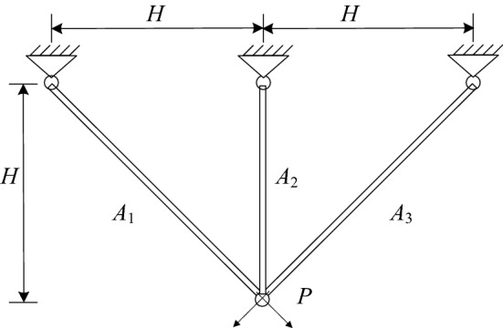
Trusses belong to one of the prefabricated concrete structures. This problem requires finding the minimum volume of the truss according to the decision variables of cross-sectional areas = = 47, as plotted in Fig. 9, the problem are described as follows:
| 6 |
Figure 9.
The three-bar truss design.
The comparison of best solution result for this problem is displayed in Table 10. As can be observed, the results given by Tsai48 are not feasible while MSCA is significantly better than the results reported in other competitive algorithms. From the comparative results, it is possible to conclude that that MSCA is work well over other methods.
Table 10.
The best solution for three-bar truss design problem.
| Algorithm | x1 | x2 | g1 | g2 | g3 | f(x) |
|---|---|---|---|---|---|---|
| Hernández49 | 0.788 | 0.408 | NA | NA | NA | 263.9 |
| Ray and Saini50 | 0.795 | 0.395 | −0.00169 | −0.26124 | −0.74045 | 264.3 |
| Raj et al.51 | 0.78976441 | 0.40517605 | −7.084 × 10⁻⁹ | −1.4675992 | −0.53240078 | 263.89671 |
| Tsai48 | 0.788 | 0.408 | 0.00082 | −0.2674 | −0.73178 | 263.68a |
| Gandomi et al.37 | 0.78867 | 0.40902 | −0.00029 | −0.26853 | −0.73176 | 263.9716 |
| MSCA | 0.788690415 | 0.408205144 | −5.2854 × 10⁻⁸ | −1.464150692 | −0.53584936 | 263.89585052 |
a means not infeasible; NA means not available. Significant values are in bold.
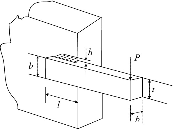
Case II: Vertical deflection I beam problem
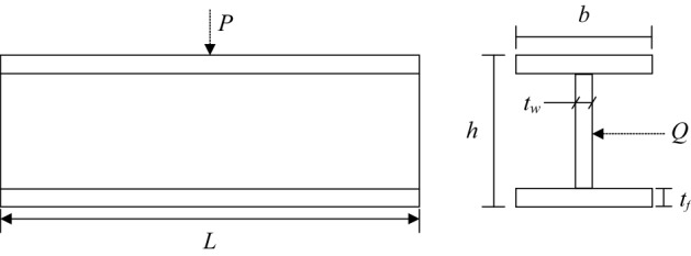
The I-beam structure is one of the design problems for prefabricated buildings with an H-shaped beam in cross-sectional form, as illustrated in Fig. 10. The objective of this problem is to minimize the vertical deflection of an I-beam while satisfying the cross-sectional area and stress constraints for a given load52. Consider the variable x = (x1, x2, x3, x4) = (h, l, t, b), the mathematical formulation of the problem is defined as follows:
| 7 |
Figure 10.
The vertical deflection of an I-beam.
The best solution and statistical results of this problem are listed in Tables 11 and 12, respectively. From Table 11, it can be seen that MSCA obtain the same objective function value as CSA and get better results than ARSM, Improved ARSM and CS methods. It is possible to conclude in Table 12 that again MSCA has noteworthy performance in all metrics.
Table 11.
The best solution for vertical deflection of an I-beam problem.
| Algorithm | h | b | tw | tf | f(x) |
|---|---|---|---|---|---|
| ARSM53 | 80 | 37.05 | 1.71 | 2.31 | 0.0157 |
| Improved ARSM53 | 79.99 | 48.42 | 0.9 | 2.4 | 0.131 |
| CS37 | 80 | 50 | 0.9 | 2.3216715 | 0.0130747 |
| CSA54 | 80 | 49.99999999 | 0.9 | 2.3217923 | 0.01307412 |
| MSCA | 80 | 50 | 0.900000012 | 2.32179198 | 0.01307412 |
Significant values are in bold.
Table 12.
Statistical result for vertical deflection of an I-beam problem.
| Algorithm | Best | Median | Mean | Worst | STD |
|---|---|---|---|---|---|
| CS37 | 0.0130747 | N/A | 0.0132165 | 0.01353646 | 1.345 × 10⁻⁴ |
| CSA54 | 0.01307412 | 0.013091263 | 0.0131397 | 0.01339323 | 9.3686 × 10⁻⁵ |
| MSCA | 0.01307412 | 0.013074137 | 0.01307415 | 0.01307421 | 2.59 × 10⁻⁸ |
Significant values are in bold.
Case III: Tension string design problem.
The main goal of this problem is to minimizes the weight of the tension string with variable include wire diameter(d), mean coil diameter(D) and the number of active coils(n), as shown in Fig. 11. the mathematical model for this problem is given as follows:
| 8 |
Figure 11.
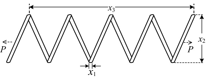
Tension string design.
The comparison results with respect to the best solution between MSCA and existing algorithms are presented in Table 13, and the related statistical information is listed in Table 14. Based on both tables, MSCA exhibits more competitive results than other methods, indicating that the proposed MSCA algorithm has strong engineering practical value.
Table 13.
The best solution for tension string design problem.
| Algorithm | x1 | x2 | x3 | f(x) |
|---|---|---|---|---|
| Belegundu55 | 0.05 | 0.3159 | 14.25 | 0.0128334 |
| Coello56 | 0.05148 | 0.351661 | 11.632201 | 0.01270478 |
| Ray and Saini50 | 0.050417 | 0.321532 | 13.979915 | 0.01306 |
| Coello and Montes57 | 0.051989 | 0.363965 | 10.890522 | 0.012681 |
| Ray and Liew 58 | 0.052160217 | 0.368158695 | 10.64844226 | 0.012669249 |
| Raj et al.51 | 0.053862 | 0.41128365 | 8.6843798 | 0.0127484 |
| Mahdavi et al.59 | 0.05115438 | 0.34987116 | 12.0764321 | 0.0126706 |
| He and Wang60 | 0.051728 | 0.357644 | 11.244543 | 0.0126747 |
| Montes and Coello61 | 0.051643 | 0.35536 | 11.397926 | 0.012698 |
| Kaveh and Talatahari62 | 0.051865 | 0.3615 | 11 | 0.0126432a |
| Coelho63 | 0.051515 | 0.352529 | 11.538862 | 0.012665a |
| Akay and Karaboga64 | 0.051749 | 0.358179 | 11.203763 | 0.012665a |
| MSCA | 0.051781993 | 0.358944836 | 11.16078852 | 0.012666807 |
a means infeasible. Significant values are in bold.
Table 14.
Statistical result for tension string design problem.
| Algorithm | Best | Median | Mean | Worst | STD |
|---|---|---|---|---|---|
| Belegundu55 | 0.0128334 | NA | NA | NA | NA |
| Coello56 | 0.01270478 | 0.01275576 | 0.0127692 | 0.01282208 | 3.9390 × 10⁻⁵ |
| Ray and Saini50 | 0.01306 | NA | 0.015526 | 0.018992 | NA |
| Coello and Montes57 | 0.012681 | NA | 0.012742 | 0.012973 | 5.9000 × 10⁻⁵ |
| Ray and Liew58 | 0.01266925 | 0.01292267 | 0.01292267 | 0.01671727 | 5.92 × 10⁻⁴ |
| He and Wang60 | 0.0126747 | NA | 0.01273 | 0.012924 | 5.1985 × 10⁻⁵ |
| Montes and Coello61 | 0.012698 | NA | 0.013461 | 0.16485 | 9.6600 × 10⁻⁴ |
| Kaveh and Talatahari62 | 0.0126432a | NA | 0.01272a | 0.012884a | 3.4888 × 10⁻⁵ |
| Coelho63 | 0.012665a | 0.012957a | 0.013524a | 0.017759a | 0.001268 |
| Akay and Karaboga64 | 0.012665a | NA | 0.012709a | NA | 0.012813 |
| MSCA | 0.01266681 | 0.01273110 | 0.01281752 | 0.01334238 | 1.90 × 10⁻⁴ |
NA means not available; a means infeasible. Significant values are in bold.
Case IV: Welded beam design problem
Welded beam design is an important part of the engineering design problem, as shown in Fig. 12, the objective is to minimize the costs of welded beam51 by selecting four variables: the thickness of weld h, length of welded joint l, width of the beam t and thickness of the beam b. The optimization model with variable is expressed as follows:
Figure 12.
Welded beam design.
Version I:
| 9 |
where the shear stress is defined as follows:
| 10 |
| 11 |
| 12 |
| 13 |
| 14 |
The MSCA is compared with four optimization methods, and the best solution and statistical results are reported in Tables 15 and 16. the results indicate that MSCA obtained the solution more accurately and more competitive than other methods.
Table 15.
The best solution for welded beam design problem on version I.
| Algorithm | x1 | x2 | x3 | x4 | f(x) |
|---|---|---|---|---|---|
| Ragsdell and Phillips65 | 0.2455 | 6.196 | 8.273 | 0.2455 | 2.385937 |
| Rao66 | 0.2455 | 6.196 | 8.273 | 0.2455 | 2.386 |
| Ray and Liew58 | 0.244438276 | 6.237967234 | 8.288576143 | 0.244566182 | 2.3854347 |
| Hwang and He67 | 0.2231 | 1.5815 | 12.8468 | 0.2245 | 2.25a |
| MSCA | 0.244249519 | 6.206365305 | 8.312174308 | 0.24432385 | 2.383286722 |
a means infeasible. Significant values are in bold.
Table 16.
Statistical result for welded beam design problem on version I.
| Algorithm | Best | Median | Mean | Worst | STD |
|---|---|---|---|---|---|
| Ragsdell and Phillips65 | 2.385937 | NA | NA | NA | NA |
| Rao66 | 2.386 | NA | NA | NA | NA |
| Ray and Liew58 | 2.3854347 | 3.0025883 | 3.2551371 | 6.3996785 | 0.959078 |
| Hwang and He67 | 2.25a | NA | 2.26a | 2.28a | NA |
| MSCA | 2.383286722 | 2.387845945 | 2.388104097 | 2.393825358 | 0.002758472 |
NA means not available; a means infeasible. Significant values are in bold.
Version II
In version II, the researchers modified the definitions of some items on the basis of version I and added a new constraint , which are defined as follows:
| 15 |
| 16 |
| 17 |
Tables 17 and 18 summarize the best solution and statistical results for version II, respectively. It can be seen from the simulation results that MSCA can still obtain convincing results with the addition of constraint of , indicating that the proposed MSCA performs better than existing studies.
Table 17.
The best solution for welded beam design problem on version II.
| Algorithm | x1 | x2 | x3 | x4 | f(x) |
|---|---|---|---|---|---|
| Coello56 | 0.2088 | 3.4205 | 8.9975 | 0.21 | 1.748309 |
| Coello and Montes57 | 0.205986 | 3.471328 | 9.020224 | 0.20648 | 1.728226 |
| He and Wang60 | 0.202369 | 3.544214 | 9.04821 | 0.205723 | 1.728024 |
| Dimopoulos68 | 0.2015 | 3.562 | 9.041398 | 0.205706 | 1.731186 |
| Mahdavi et al.59 | 0.20573 | 3.47049 | 9.03662 | 0.20573 | 1.7248 |
| Montes et al.69 | 0.20573 | 3.470489 | 9.036624 | 0.20573 | 1.724852 |
| Montes and Coello61 | 0.199742 | 3.61206 | 9.0375 | 0.206082 | 1.7373 |
| Cagnina et al.70 | 0.205729 | 3.470488 | 9.036624 | 0.205729 | 1.724852 |
| Kaveh and Talatahari71 | 0.205729 | 3.469875 | 9.036805 | 0.205765 | 1.724849 |
| Kaveh and Talatahari62 | 0.2057 | 3.471131 | 9.036683 | 0.205731 | 1.724918 |
| Gandomi et al.72 | 0.2015 | 3.562 | 9.0414 | 0.2057 | 1.73121 |
| Mehta and Dasgupta73 | 0.20572885 | 3.47050567 | 9.03662392 | 0.20572964 | 1.724855 |
| Akay and Karaboga64 | 0.20573 | 3.470489 | 9.036624 | 0.20573 | 1.724852 |
| MSCA | 0.205187143 | 3.266067065 | 9.03380051 | 0.205913062 | 1.69710013 |
Significant values are in bold.
Table 18.
Statistical result for welded beam design problem on version II.
| Algorithm | Best | Median | Mean | Worst | STD |
|---|---|---|---|---|---|
| Coello56 | 1.748309 | NA | 1.771973 | 1.785835 | 0.01122 |
| Coello and Montes57 | 1.728226 | NA | 1.792654 | 1.993408 | 0.07471 |
| He and Wang60 | 1.728024 | NA | 1.748831 | 1.782143 | 0.012926 |
| Dimopoulos68 | 1.731186 | NA | NA | NA | NA |
| Montes et al.69 | 1.724852 | NA | 1.725 | NA | 1.0 × 10⁻¹⁵ |
| Montes and Coello61 | 1.7373 | NA | 1.81329 | 1.994651 | 0.0705 |
| Cagnina et al.70 | 1.724852 | NA | 2.0574 | NA | 0.2154 |
| Kaveh and Talatahari71 | 1.724849 | NA | 1.727564 | 1.759522 | 0.008254 |
| Kaveh and Talatahari62 | 1.724918 | NA | 1.729752 | 1.775961 | 0.0092 |
| Gandomi et al.72 | 1.7312065 | NA | 1.878656 | 2.3455793 | 0.2677989 |
| Mehta and Dasgupta73 | 1.724855 | 1.724861 | 1.724865 | 1.72489 | NA |
| Akay and Karaboga64 | 1.724852 | NA | 1.741913 | NA | 0.031 |
| MSCA | 1.69710013 | 1.700828362 | 1.70209677 | 1.722162002 | 0.005815737 |
NA means not available. Significant values are in bold.
Case V: Gear train design problem
The gear train design problem was first proposed by Sandgren74 as an unconstrained optimization problem, presented in Fig. 13. The task of the problem is to find the best variable vector to minimize cost of gear ratio. The optimization formula is given as follows:
| 18 |
where gear ratio = .
Figure 13.
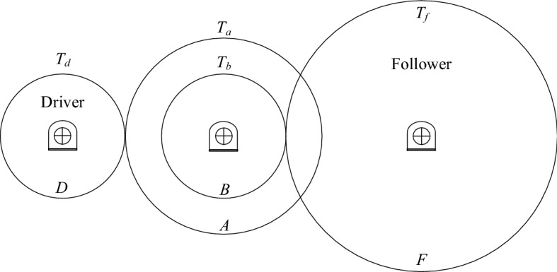
Gear train design.
To address this issue, MSCA was compared with several classical methods, and the best solutions recorded for MSCA and other literature results are listed in Table 19. On the other hand, the corresponding statistical results are represented in Table 20. The both tables show that MSCA provides more stable and accurate solutions than other methods.
Table 19.
The best solution for gear train design problem.
| Algorithm | Td(x1) | Tb(x2) | Ta(x3) | Tf(x4) | Gear ratio | f(x) |
|---|---|---|---|---|---|---|
| Sandgren75 | 18 | 22 | 45 | 60 | 0.146667 | 5.712 × 10⁻⁶ |
| Kannan and Kramer76 | 13 | 15 | 33 | 41 | 0.144124 | 2.146 × 10⁻⁸ |
| Deb and Goyal77 | 19 | 16 | 49 | 43 | 0.144281 | 2.701 × 10⁻¹² |
| Gandomi et al.37 | 19 | 16 | 43 | 49 | 0.144281 | 2.701 × 10⁻¹² |
| Garg78 | 19 | 16 | 43 | 49 | 0.14428096 | 2.7008571 × 10⁻¹² |
| MSCA | 19 | 16 | 43 | 49 | 0.14428096 | 2.7008571 × 10⁻¹² |
Significant values are in bold.
Table 20.
Statistical result for gear train design problem.
| Algorithm | Best | Median | Mean | Worst | STD |
|---|---|---|---|---|---|
| Gandomi et al.78 | 2.7009 × 10⁻¹² | NA | 1.9841 × 10⁻⁹ | 2.3576 × 10⁻⁹ | 3.5546 × 10⁻⁹ |
| Garg37 | 2.7008571 × 10⁻¹² | 9.9215795 × 10⁻¹⁰ | 1.2149276 × 10⁻⁹ | 3.2999231 × 10⁻⁹ | 8.77 × 10⁻¹⁰ |
| MSCA | 2.7008571 × 10⁻¹² | 2.3078157 × 10⁻¹¹ | 4.8092363 × 10⁻¹¹ | 3.0675559 × 10⁻¹⁰ | 7.4270038 × 10⁻¹¹ |
NA means not available. Significant values are in bold.
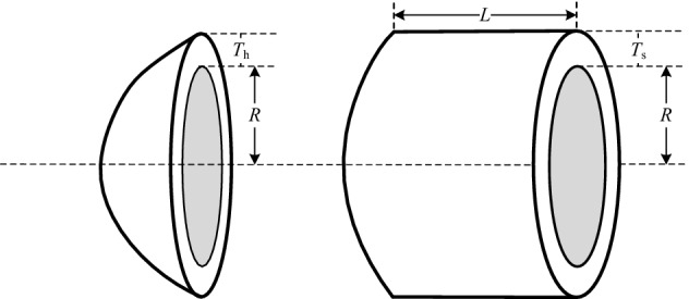
Case VI: Pressure vessel design problem
IN this problem, shown in Fig. 14, the task is to minimize the total cost of the vessel with decision vector = = 79. The optimization model is constructed as follows:
| 19 |
Figure 14.
Pressure vessel design.
Version I:
| 20 |
The best results and statistical results for version I are reported in Tables 21 and 22, respectively. As can be seen from Table 21, MCSA obtain more objective results than other literature, and from Table 22, MCSA further obtains a more concentrated solution distribution, demonstrating the superior search performance of the proposed method.
Table 21.
The best solution for pressure vessel design problem on version I.
| Algorithm | x1 | x2 | x3 | x4 | f(x) |
|---|---|---|---|---|---|
| Sandgren74 | 1.125 | 0.625 | 47.7 | 117.701 | 8129.1036 |
| Kannan and Kramer80 | 1.125 | 0.625 | 58.291 | 43.69 | 7198.0428 |
| Coello and Montes57 | 0.8125 | 0.4375 | 42.097398 | 176.65405 | 6059.946 |
| He and Wang60 | 0.8125 | 0.4375 | 42.091266 | 176.7465 | 6061.0777 |
| Montes and Coello61 | 0.8125 | 0.4375 | 42.098087 | 176.640518 | 6059.7456 |
| Coelho63 | 0.8125 | 0.4375 | 42.0984 | 176.6372 | 6059.7208 |
| He et al.81 | 0.8125 | 0.4375 | 42.098445 | 176.636595 | 6059.7143 |
| Montes et al.69 | 0.8125 | 0.4375 | 42.098446 | 176.636047 | 6059.70166 |
| Gandomi et al.37 | 0.8125 | 0.4375 | 42.0984456 | 176.6365958 | 6059.714335 |
| Akay and Karaboga64 | 0.8125 | 0.4375 | 42.098446 | 176.636596 | 6059.714339 |
| MSCA | 0.780583407 | 0.3917558 | 40.4190779 | 198.964126 | 5917.509793 |
Significant values are in bold.
Table 22.
Statistical result for pressure vessel design problem on version I.
| Algorithm | Best | Median | Mean | Worst | STD |
|---|---|---|---|---|---|
| Sandgren74 | 8129.1036 | NA | N/A | N/A | N/A |
| Kannan and Kramer80 | 7198.0428 | NA | N/A | N/A | N/A |
| Coello and Montes57 | 6059.9463 | NA | 6177.2533 | 6469.322 | 130.9297 |
| Montes and Coello61 | 6059.7456 | NA | 6850.0049 | 7332.8798 | 426 |
| Gandomi et al.37 | 6059.714 | NA | 6447.736 | 6495.347 | 502.693 |
| Coelho63 | 6059.7208 | 6257.5943 | 6440.3786 | 7544.4925 | 448.4711 |
| He et al.81 | 6059.7143 | NA | 6289.92881 | NA | 305.78 |
| Akay and Karaboga64 | 6059.714339 | NA | 6245.30814 | NA | 205 |
| MSCA | 5917.509793 | 5994.4224 | 6029.24374 | 6396.551211 | 113.2470944 |
NA means not available. Significant values are in bold.
Version II:
| 21 |
In version II, the upper bound of the decision variable x4 is set as 240, the best results and statistical results summarized by MSCA and control methods for version II in Tables 23 and 24, respectively. Analysis from both tables, MSCA reveals better performance than the existing studies. The comparison results further prove that MCSA has better feasibility in engineering than the other approaches.
Table 23.
The best solution for pressure vessel design problem on version II.
| Algorithm | x1 | x2 | x3 | x4 | f(x) |
|---|---|---|---|---|---|
| Dimopoulos68 | 0.75 | 0.375 | 38.8601 | 221.36549 | 5850.38306 |
| Mahdavi et al.59 | 0.75 | 0.375 | 38.8601 | 221.36553 | 5849.76169 |
| Gandomi et al.72 | 0.75 | 0.375 | 38.8601 | 221.36547 | 5850.38306 |
| MSCA | 0.73822151 | 0.36818507 | 38.16830296 | 232.73616127 | 5849.52062 |
Significant values are in bold.
Table 24.
Statistical result for pressure vessel design problem on version II.
| Algorithm | Best | Median | Mean | Worst | STD |
|---|---|---|---|---|---|
| Dimopoulos68 | 5850.383060 | NA | NA | NA | NA |
| Mahdavi et al.59 | 5849.761700 | NA | NA | NA | NA |
| Gandomi et al.72 | 5850.383060 | NA | 5937.337900 | 6258.968250 | 164.547470 |
| MSCA | 5849.520622 | 5919.655417 | 5944.332084 | 6217.813607 | 87.356362 |
NA means not available. Significant values are in bold.
Conclusion
In this article, the position update adjustment strategy and Levy random walk mutation mechanism were adopted into the original SCA to create the proposed MCSA. The position update adjustment strategy considers the swarm search for potentially better solutions around the current individual and the global optimal individual, effectively expanding the search and improving the convergence speed of the original SCA. And the Levy random walk mutation mechanism effectively increases the original SCA diversity to ensure that the SCAs jump out of the local optimal position and improve the search accuracy.
For qualitative analysis of proposed method (MSCA), it has been passed two levels of benchmark test suites—the classic and the IEEE CEC2017 function. box plots and convergence curves were employed to verify the performance of robustness and convergence. In addition, Wilcoxon signed-rank test and ranksum test were adopted to verify statistical significance. The experimental results show that MSCA is able to balance the exploration and exploitation process. Finally, MSCA is used to solve six complex real-world engineering design problems, and the comparison with the results of several other state-of-the-art methods proves that the proposed method can achieve competitive results. Based on the convincing results obtained from existing research, in the future we will try to apply the proposed method to image recognition and time series forecasting problems.
Acknowledgements
The writers would like to thank editors and reviewers for their valuable comments and suggestions.
Author contributions
Conceptualization, C.S.; writing—review and editing, C.S.; validation, T.Z.; data curation, T.Z.; writing—original draft preparation, T.Z. methodology, S.L.; software, S.L.; All authors read and agreed to the published version of the manuscript.
Data availability
The data that support the findings of this study are available from the corresponding author upon request. There are no restrictions on data availability.
Competing interests
The authors declare no competing interests.
Footnotes
Publisher's note
Springer Nature remains neutral with regard to jurisdictional claims in published maps and institutional affiliations.
References
- 1.Beheshti Z, Shamsuddin SMH. A review of population-based meta-heuristic algorithms. Int. J. Adv. Soft Comput. Appl. 2013;5(1):1–35. [Google Scholar]
- 2.Mirjalili S. SCA: A sine cosine algorithm for solving optimization problems. Knowl-Based Syst. 2016;96:120–133. doi: 10.1016/j.knosys.2015.12.022. [DOI] [Google Scholar]
- 3.Kaveh, A. Advances in metaheuristic algorithms for optimal design of structures: Springer (2014).
- 4.Mirjalili S, Lewis A. The whale optimization algorithm. Adv. Eng. Softw. 2016;95:51–67. doi: 10.1016/j.advengsoft.2016.01.008. [DOI] [Google Scholar]
- 5.Deb K. An introduction to genetic algorithms. Sadhana. 1999;24:293–315. doi: 10.1007/BF02823145. [DOI] [Google Scholar]
- 6.Deng W, Shang S, Cai X, Zhao H, Song Y, Xu J. An improved differential evolution algorithm and its application in optimization problem. Soft Comput. 2021;25:5277–5298. doi: 10.1007/s00500-020-05527-x. [DOI] [Google Scholar]
- 7.Beyer, H. G., & Sendhoff, B. Evolution strategies for robust optimization. In 2006 IEEE International Conference on Evolutionary Computation (pp. 1346-1353) IEEE. (2006).
- 8.Rashedi E, Nezamabadi-Pour H, Saryazdi S. GSA: A gravitational search algorithm. Inform. Sci. 2009;179:2232–2248. doi: 10.1016/j.ins.2009.03.004. [DOI] [Google Scholar]
- 9.Kaveh A, Talatahari S. A novel heuristic optimization method: Charged system search. Acta Mech. 2010;213:267–289. doi: 10.1007/s00707-009-0270-4. [DOI] [Google Scholar]
- 10.Dorigo M, Birattari M, Stutzle T. Ant colony optimization. IEEE Comput. Intell. Mag. 2006;1(4):28–39. doi: 10.1109/MCI.2006.329691. [DOI] [Google Scholar]
- 11.Marini F, Walczak B. Particle swarm optimization (PSO). A Tutorial. Chemometr. Intell. Lab. 2015;149:153–165. doi: 10.1016/j.chemolab.2015.08.020. [DOI] [Google Scholar]
- 12.Heidari AA, Mirjalili S, Faris H, Aljarah I, Mafarja M, Chen H. Harris hawks optimization: Algorithm and applications. Futur. Gener. Comput. Syst. 2019;97:849–872. doi: 10.1016/j.future.2019.02.028. [DOI] [Google Scholar]
- 13.Sadoun AM, Najjar IR, Alsoruji GS, Wagih A, Abd Elaziz M. Utilizing a long short-term memory algorithm modified by dwarf mongoose optimization to predict thermal expansion of Cu-Al2O3 nanocomposites. Mathematics. 2022;10(7):1050. doi: 10.3390/math10071050. [DOI] [Google Scholar]
- 14.Agushaka JO, Ezugwu AE, Abualigah L. Dwarf mongoose optimization algorithm. Comput. Methods Appl. Mech. Eng. 2022;391:114570. doi: 10.1016/j.cma.2022.114570. [DOI] [Google Scholar]
- 15.Al-Shourbaji I, Helian N, Sun Y, Alshathri S, Abd Elaziz M. Boosting ant colony optimization with reptile search algorithm for churn prediction. Mathematics. 2022;10(7):1031. doi: 10.3390/math10071031. [DOI] [Google Scholar]
- 16.Abualigah L, Abd Elaziz M, Sumari P, Geem ZW, Gandomi AH. Reptile search algorithm (RSA): A nature-inspired meta-heuristic optimizer. Expert Syst. Appl. 2022;191:116158. doi: 10.1016/j.eswa.2021.116158. [DOI] [Google Scholar]
- 17.Oyelade ON, Ezugwu AE. A bioinspired neural architecture search based convolutional neural network for breast cancer detection using histopathology images. Sci. Rep.-UK. 2021;11:1–28. doi: 10.1038/s41598-021-98978-7. [DOI] [PMC free article] [PubMed] [Google Scholar]
- 18.Oyelade ON, Ezugwu AES, Mohamed TIA, Abualigah L. Ebola optimization search algorithm: A new nature-inspired metaheuristic optimization algorithm. IEEE Access. 2022;10:16150–16177. doi: 10.1109/ACCESS.2022.3147821. [DOI] [Google Scholar]
- 19.Xing Q, Wang J, Lu H, Wang S. Research of a novel short-term wind forecasting system based on multi-objective Aquila optimizer for point and interval forecast. Energ. Convers. Manage. 2022;263:115583. doi: 10.1016/j.enconman.2022.115583. [DOI] [Google Scholar]
- 20.Abualigah L, Yousri D, Abd Elaziz M, Ewees AA, Al-Qaness MA, Gandomi AH. Aquila Optimizer: A novel meta-heuristic optimization algorithm. Comput. Indus. Eng. 2021;157:107250. doi: 10.1016/j.cie.2021.107250. [DOI] [Google Scholar]
- 21.Guha, R., Ghosh, K.K., Bera, S.K., Sarkar, R. & Mirjalili, S. Discrete equilibrium optimizer combined with simulated annealing for feature selection. Res. Square (2022).
- 22.Hashim FA, Hussien AG. Snake optimizer: A novel meta-heuristic optimization algorithm. Knowl.-Based Syst. 2022;242:108320. doi: 10.1016/j.knosys.2022.108320. [DOI] [Google Scholar]
- 23.Hussien AG, Abualigah L, Abu Zitar R, Hashim FA, Amin M, Saber A, Gandomi AH. Recent advances in harris hawks optimization: A comparative study and applications. Electronics. 2022;11(12):1919. doi: 10.3390/electronics11121919. [DOI] [Google Scholar]
- 24.Wang S, Hussien AG, Jia H, Abualigah L, Zheng R. Enhanced remora optimization algorithm for solving constrained engineering optimization problems. Mathematics. 2022;10(10):1696. doi: 10.3390/math10101696. [DOI] [Google Scholar]
- 25.Mostafa, R. R., Hussien, A. G., Khan, M. A., Kadry, S., & Hashim, F. A. Enhanced coot optimization algorithm for dimensionality reduction. In: 2022 Fifth International Conference of Women in Data Science at Prince Sultan University (WiDS PSU) (pp. 43-48). IEEE (2022).
- 26.Yu H, Jia H, Zhou J, Hussien A. Enhanced aquila optimizer algorithm for global optimization and constrained engineering problems. Math. Biosci. Eng. 2022;19(12):14173–14211. doi: 10.3934/mbe.2022660. [DOI] [PubMed] [Google Scholar]
- 27.Zheng R, Hussien AG, Jia HM, Abualigah L, Wang S, Wu D. An improved wild horse optimizer for solving optimization problems. Mathematics. 2022;10(8):1311. doi: 10.3390/math10081311. [DOI] [Google Scholar]
- 28.Hussien AG, Amin M. A self-adaptive Harris Hawks optimization algorithm with opposition-based learning and chaotic local search strategy for global optimization and feature selection. Int. J. Mach. Learn. Cyb. 2022;13:309–336. doi: 10.1007/s13042-021-01326-4. [DOI] [Google Scholar]
- 29.Singh S, Singh H, Mittal N, Singh H, Hussien AG, Sroubek F. A feature level image fusion for Night-Vision context enhancement using Arithmetic optimization algorithm based image segmentation. Expert Syst Appl. 2022;209:118272. doi: 10.1016/j.eswa.2022.118272. [DOI] [Google Scholar]
- 30.Abualigah L, Diabat A. Advances in sine cosine algorithm: A comprehensive survey. Artif. Intell. Rev. 2021;54:2567–2608. doi: 10.1007/s10462-020-09909-3. [DOI] [PMC free article] [PubMed] [Google Scholar]
- 31.Abd Elaziz M, Oliva D, Xiong S. An improved opposition-based sine cosine algorithm for global optimization. Expert Syst. Appl. 2017;90:484–500. doi: 10.1016/j.eswa.2017.07.043. [DOI] [Google Scholar]
- 32.Neggaz N, Ewees AA, Elaziz MA, Mafarja M. Boosting salp swarm algorithm by sine cosine algorithm and disrupt operator for feature selection. Expert Syst. Appl. 2020;145:113103. doi: 10.1016/j.eswa.2019.113103. [DOI] [Google Scholar]
- 33.El-Kenawy ESM, Mirjalili S, Ghoneim SS, Eid MM, El-Said M, Khan ZS, Ibrahim A. Advanced ensemble model for solar radiation forecasting using sine cosine algorithm and newton’s laws. IEEE Access. 2021;9:115750–115765. doi: 10.1109/ACCESS.2021.3106233. [DOI] [Google Scholar]
- 34.Gupta S, Deep K, Mirjalili S, Kim JH. A modified Sine Cosine Algorithm with novel transition parameter and mutation operator for global optimization. Expert Syst. Appl. 2020;154:113395. doi: 10.1016/j.eswa.2020.113395. [DOI] [Google Scholar]
- 35.Li Y, Zhao Y, Liu J. Dynamic sine cosine algorithm for large-scale global optimization problems. Expert Syst. Appl. 2021;177:114950. doi: 10.1016/j.eswa.2021.114950. [DOI] [Google Scholar]
- 36.Gupta S, Deep K. A hybrid self-adaptive sine cosine algorithm with opposition based learning. Expert Syst. Appl. 2019;119:210–230. doi: 10.1016/j.eswa.2018.10.050. [DOI] [Google Scholar]
- 37.Gandomi AH, Yang XS, Alavi AH. Cuckoo search algorithm: A metaheuristic approach to solve structural optimization problems. Eng. Comput.-Germany. 2013;29:17–35. doi: 10.1007/s00366-011-0241-y. [DOI] [Google Scholar]
- 38.Yao X, Liu Y, Lin G. Evolutionary programming made faster. IEEE T Evolut. Comput. 1999;3:82–102. doi: 10.1109/4235.771163. [DOI] [Google Scholar]
- 39.Wu, G., Mallipeddi, R. & Suganthan, P.N. Problem definitions and evaluation criteria for the CEC 2017 competition on constrained real-parameter optimization. National University of Defense Technology, Changsha, Hunan, PR China and Kyungpook National University, Daegu, South Korea and Nanyang Technological University, Singapore, Technical Report (2017).
- 40.Whitley D. A genetic algorithm tutorial. Stat. Comput. 1994;4:65–85. doi: 10.1007/BF00175354. [DOI] [Google Scholar]
- 41.Houssein, E.H., Gad, A.G. & Wazery, Y.M. Jaya Algorithm and Applications: A Comprehensive Review. In: Razmjooy N, Ashourian M, Foroozandeh Z, ''editors'. Metaheuristics and Optimization in Computer and Electrical Engineering. Cham: Springer International Publishing; 3–24 (2021).
- 42.Mirjalili S. The ant lion optimizer. Adv. Eng. Softw. 2015;83:80–98. doi: 10.1016/j.advengsoft.2015.01.010. [DOI] [Google Scholar]
- 43.Abualigah L. Multi-verse optimizer algorithm: A comprehensive survey of its results, variants, and applications. Neural Comput. Appl. 2020;32:12381–12401. doi: 10.1007/s00521-020-04839-1. [DOI] [Google Scholar]
- 44.Mirjalili S, Mirjalili SM, Lewis A. Grey wolf optimizer. Adv. Eng. Softw. 2014;69:46–61. doi: 10.1016/j.advengsoft.2013.12.007. [DOI] [Google Scholar]
- 45.Mirjalili S, Gandomi AH, Mirjalili SZ, Saremi S, Faris H, Mirjalili SM. Salp Swarm Algorithm: A bio-inspired optimizer for engineering design problems. ADV ENG SOFTW. 2017;114:163–191. doi: 10.1016/j.advengsoft.2017.07.002. [DOI] [Google Scholar]
- 46.Abualigah L, Diabat A, Mirjalili S, Abd Elaziz M, Gandomi AH. The arithmetic optimization algorithm. Comput. Method Appl. M. 2021;376:113609. doi: 10.1016/j.cma.2020.113609. [DOI] [Google Scholar]
- 47.Nowacki, H. Optimization in pre-contract ship design. (1973).
- 48.Tsai JFA. Global optimization of nonlinear fractional programming problems in engineering design. Eng. Optimiz. 2005;37:399–409. doi: 10.1080/03052150500066737. [DOI] [Google Scholar]
- 49.Hernendez, S. Multiobjective structural optimization. Geo. Opt. Tech. Struct. Design. 341–362 (1994).
- 50.Ray T, Saini P. Engineering design optimization using a swarm with an intelligent information sharing among individuals. Eng. Optimiz. 2001;33:735–748. doi: 10.1080/03052150108940941. [DOI] [Google Scholar]
- 51.Raj KH, Sharma RS, Mishra GS, Dua A, Patvardhan C. An evolutionary computational technique for constrained optimisation in engineering design. J. Inst. Eng. (India): Mech. Eng. Division. 2005;86:121–128. [Google Scholar]
- 52.Gold, S. & Krishnamurty, S. Trade-offs in robust engineering design. (American Society of Mechanical Engineers, 1997), pp. V2T-V29T.
- 53.Wang GG. Adaptive response surface method using inherited Latin hypercube design points. J. Mech. Des., Trans. ASME. 2003;125:210–220. doi: 10.1115/1.1561044. [DOI] [Google Scholar]
- 54.Feng ZK, Niu WJ, Liu S. Cooperation search algorithm: A novel metaheuristic evolutionary intelligence algorithm for numerical optimization and engineering optimization problems. Appl. Soft Comput. 2021;98:106734. doi: 10.1016/j.asoc.2020.106734. [DOI] [Google Scholar]
- 55.Belegundu, A.D. A study of mathematical programming methods for structural optimization. A Study of Mathematical Programming Methods for Structural Optimization (1982).
- 56.Coello Coello CA. Use of a self-adaptive penalty approach for engineering optimization problems. Comput. Ind. 2000;41:113–127. doi: 10.1016/S0166-3615(99)00046-9. [DOI] [Google Scholar]
- 57.Coello Coello CA, Montes EM. Constraint-handling in genetic algorithms through the use of dominance-based tournament selection. Adv. Eng. Inform. 2002;16:193–203. doi: 10.1016/S1474-0346(02)00011-3. [DOI] [Google Scholar]
- 58.Ray T, Liew KM. Society and civilization: An optimization algorithm based on the simulation of social behavior. IEEE T Evolut. Comput. 2003;7:386–396. doi: 10.1109/TEVC.2003.814902. [DOI] [Google Scholar]
- 59.Mahdavi M, Fesanghary M, Damangir E. An improved harmony search algorithm for solving optimization problems. Appl. Math. Comput. 2007;188:1567–1579. [Google Scholar]
- 60.He Q, Wang L. An effective co-evolutionary particle swarm optimization for constrained engineering design problems. Eng. Appl. Artif. Intel. 2007;20:89–99. doi: 10.1016/j.engappai.2006.03.003. [DOI] [Google Scholar]
- 61.Mezura-Montes E, Coello CAC. An empirical study about the usefulness of evolution strategies to solve constrained optimization problems. Int. J Gen. Syst. 2008;37:443–473. doi: 10.1080/03081070701303470. [DOI] [Google Scholar]
- 62.Kaveh A, Talatahari S. An improved ant colony optimization for constrained engineering design problems. Eng. Comput. (Swansea, Wales). 2010;27:155–182. doi: 10.1108/02644401011008577. [DOI] [Google Scholar]
- 63.Coelho LDS. Gaussian quantum-behaved particle swarm optimization approaches for constrained engineering design problems. Expert Syst. Appl. 2010;37:1676–1683. doi: 10.1016/j.eswa.2009.06.044. [DOI] [Google Scholar]
- 64.Akay B, Karaboga D. Artificial bee colony algorithm for large-scale problems and engineering design optimization. J. Intell. Manuf. 2012;23:1001–1014. doi: 10.1007/s10845-010-0393-4. [DOI] [Google Scholar]
- 65.Ragsdell KM, Phillips DT. Optimal design of a class of welded structures using geometric programming. J. Manuf. Sci. E. T. ASME. 1976;98:1021–1025. [Google Scholar]
- 66.Rao, S.S. Engineering optimization: Theory and practice (2019).
- 67.Hwang SF, He RS. A hybrid real-parameter genetic algorithm for function optimization. Adv. Eng. Inform. 2006;20:7–21. doi: 10.1016/j.aei.2005.09.001. [DOI] [Google Scholar]
- 68.Dimopoulos GG. Mixed-variable engineering optimization based on evolutionary and social metaphors. Comput. Method Appl. M. 2007;196:803–817. doi: 10.1016/j.cma.2006.06.010. [DOI] [Google Scholar]
- 69.Mezura-Montes E, Coello CAC, Velázquez-Reyes J, Muñoz-Dávila L. Multiple trial vectors in differential evolution for engineering design. Eng. Optimiz. 2007;39:567–589. doi: 10.1080/03052150701364022. [DOI] [Google Scholar]
- 70.Cagnina LC, Esquivel SC, Coello Coello CA. Solving engineering optimization problems with the simple constrained particle swarm optimizer. Informatica (Ljubljana). 2008;32:319–326. [Google Scholar]
- 71.Kaveh A, Talatahari S. Engineering optimization with hybrid particle swarm and ant colony optimization. Asian J. Civil Eng. 2009;10:611–628. [Google Scholar]
- 72.Gandomi AH, Yang XS, Alavi AH. Mixed variable structural optimization using Firefly Algorithm. Comput. Struct. 2011;89:2325–2336. doi: 10.1016/j.compstruc.2011.08.002. [DOI] [Google Scholar]
- 73.Mehta VK, Dasgupta B. A constrained optimization algorithm based on the simplex search method. Eng. Optimiz. 2012;44:537–550. doi: 10.1080/0305215X.2011.598520. [DOI] [Google Scholar]
- 74.Sandgren, E. Nonlinear integer and discrete programming in mechanical design. In Advances in Design Automation - 1988, (Publ by American Soc of Mechanical Engineers (ASME), New York, NY, United States Kissimmee, FL, USA, 1988), pp. 95–105.
- 75.Sandgren, E. Nonlinear Integer and Discrete Programming in Mechanical Design. ASME 1988 Design Technology Conferences. 95–105 (1988).
- 76.Kannan BK, Kramer SN. An augmented lagrange multiplier based method for mixed integer discrete continuous optimization and its applications to mechanical design. J. Mech. Design. 1994;116:405–411. doi: 10.1115/1.2919393. [DOI] [Google Scholar]
- 77.Deb K, Goyal M. A combined genetic adaptive search (GeneAS) for engineering design. Comput. Sci. Inf. 1996;26:30–45. [Google Scholar]
- 78.Garg H. A hybrid GSA-GA algorithm for constrained optimization problems. Inform. Sci. 2019;478:499–523. doi: 10.1016/j.ins.2018.11.041. [DOI] [Google Scholar]
- 79.Kannan, B.K., Kramer S.N. An augmented Lagrange multiplier based method for mixed integer discrete continuous optimization and its applications to mechanical design. (1994).
- 80.Kannan BK, Kramer SN. An augmented lagrange multiplier based method for mixed integer discrete continuous optimization and its applications to mechanical design. J. Mech. Des., Trans. ASME. 1994;116:405–411. doi: 10.1115/1.2919393. [DOI] [Google Scholar]
- 81.He S, Prempain E, Wu QH. An improved particle swarm optimizer for mechanical design optimization problems. Eng. Optimiz. 2004;36:585–605. doi: 10.1080/03052150410001704854. [DOI] [Google Scholar]
Associated Data
This section collects any data citations, data availability statements, or supplementary materials included in this article.
Data Availability Statement
The data that support the findings of this study are available from the corresponding author upon request. There are no restrictions on data availability.