Study on inversion method of wall erosion information of on-orbit Hall thruster based on low-frequency oscillation signals and neural networks

Abstract

Hall thrusters function as power plants on spacecraft, and its development is crucial for the aerospace industry. The wall erosion of the on-orbit Hall thruster cannot be measured by the control center through ground measurement, but can obtain the discharge current low-frequency oscillation data. Therefore, this study proposes an inversion method to obtain the wall erosion information based on low-frequency oscillation signals and neural networks. Firstly, we use an improved one-dimensional quasi-neutral dynamic fluid mathematical model to build a low-frequency oscillation simulation platform which obtains the corresponding data by varying the cross-sectional area. Secondly, a nonlinear neural network model is established based on the obtained low-frequency oscillation data to invert the wall erosion information. The training function, transfer function, number of hidden layer nodes, and other parameters affecting the results are analyzed and the best model parameters are obtained. The Elman neural network is established and compared with the BP neural network and RBF neural network. The training results of the Elman neural network algorithm present small and stable errors, and the results of multiple predictions remain consistent. The root means square error, average absolute error, and average absolute percentage are 0.0084, 0.0637, and 0.045%, respectively.

Hall thruster; Low-frequency oscillation; Neural network; Wall erosion; Information inversion.

1. Introduction

Electric propulsion devices which can provide power for spacecraft are being developed with the continuous development of space technology. Hall thrusters have become one of most the preferred electric propulsion devices for spacecraft owing to their high efficiency, specific impulse, and long life [1]. Wall erosion is the main factor affecting the life as well as the low-frequency oscillations of Hall thrusters [2]. Low-frequency oscillation is an inherent property of the on-orbit motion of Hall thrusters. This oscillation can cause significant changes in the voltage with a change in the loop current [3].

Extensive research has been conducted on the wall erosion of thruster channels. However, the existing studies were focused on ground-life test measurements and numerical simulation methods. The ground experiment directly reflected the wall erosion, and the life of the thruster was obtained at the end of the experiment. However, the life experiment is expensive and consumes a long time. The numerical simulation of the wall-erosion process of the thruster was performed using a semi-empirical formula which was obtained by fitting the existing experimental data. This method is inexpensive and relatively less time-consuming; however, it does not concur with actual measurements. Abgaryan et al. developed an equivalent ion source model and provided an empirical formula to calculate the wall life based on experimental data and analysis [4]. Baranov et al. also developed a wall erosion prediction formula using wall evolution and ion motion equations [5]. Sommier et al. wrote a set of Hall thruster simulation programs based on the two-dimensional particle-in-cell (PIC) model and conducted a series of studies on Hall thruster wall erosion using these programs [6]. Szabo proposed a model acceleration method to reduce the mass of heavy particles and increase the dielectric constant and developed a full-particle-in-cell simulation method based on this method [7]. Cho et al. proposed an acceleration method which only increases the electron mass, and performed a whole-particle wall corrosion simulation based on this method [8].

The prediction of the wall erosion of Hall thrusters depends on the formula and empirical parameters. This method faces various drawbacks and does not consider the changes in the parameters during the process. The control center cannot measure the wall erosion of the on-orbit Hall thruster using ground measurement but can obtain the low-frequency oscillation data of the discharge current. A neural network can be used to establish a complex nonlinear model which can train and predict unknown and unmeasured data using low-frequency oscillation data. The neural network can input data and classify the output through the low-frequency oscillation data of the discharge current. The neural network was summarized based on these data after running all the sample data. Subsequently, a neural network was used for testing based on the test samples in the test set. A neural network model is successfully established if the test accuracy is high. The wall erosion was then inversed using a neural network [9].

In this study, an improved one-dimensional quasi-neutral fluid model was developed to obtain the sample data of the low-frequency oscillation discharge current by varying the cross-sectional area. The sample set was divided in a ratio of 3:1 and three sets of samples were used to train the nonlinear neural networks which are then used to predict the wall erosion. The remaining samples were used as tests and were compared with the predicted values of the neural network.

2. Improvement of one-dimensional quasi-neutral fluid model

2.1. One-dimensional quasi-neutral fluid model

A one-dimensional quasi-neutral fluid model was used to obtain the low-frequency oscillation current data [10, 11, 12]. The electron and ion densities in the channel are considered to be equal assuming that the plasma in the discharge channel is quasi-neutral [13]. The discharge channel direction was set as the x-axis, with x = 0 at the anode entrance, and x = L at the channel exit. The continuous equation of atomic motion is given as (Eqn 1) [14, 15, 16]:

$$\frac{\partial n_a}{\partial t}+V_{\mathrm{a}}\frac{\partial n_a}{\partial x}=-\beta n{n}_a$$ (1)

where $V_{\mathrm{a}}$ denotes the atomic velocity, $V_{\mathrm{a}}$ is a constant greater than 0, (in m/s), $\beta$ denotes the ionization rate (in m³/s), and denotes the atomic density (in m⁻³).

The model equation also includes the ion continuity equation, which is given as (Eqn 2):

$$\frac{\partial n}{\partial t}+\frac{\partial \mathrm{n}V}{\partial x}=\beta n{n}_a$$ (2)

where V denotes the ion velocity (in m/s).

The ion momentum equation is given as (Eqn 3):

$$\frac{\partial nV}{\partial t}+\frac{\partial n{V}^2}{\partial x}=\frac{en}{M}E+\beta n{n}_a{V}_{\mathrm{a}}$$ (3)

where e denotes the basic charge (C), E denotes the electric field strength (V/m), and M denotes the mass of a single ion or an atom.

The electric field changes dynamically. The form of electron conduction is used to introduce a changing electric field. Therefore, the conduction of electrons is considered to be related only to the strength of the radial magnetic field, and can be obtained as (Eqn 4):

$$E=\frac{I/A-enV}{\sigma \left(\mathrm{x}\right)}$$ (4)

where A denotes the cross-sectional area of the discharge channel (in m²) and $\sigma \left(\mathrm{x}\right)$ denotes the electronic conductivity (in S/m).

The discharge circuit equation is given as (Eqn 5):

$$L_{\mathrm{c}}\frac{\mathrm{d}I}{\mathrm{d}\mathrm{t}}+RI+{\int }_0^{L}E\mathrm{d}\mathrm{x}=U$$ (5)

where $L_{\mathrm{c}}$ represents the inductance, whose unit is H, R represents the resistance, whose unit is $\Omega$, and U represents the power supply voltage, whose unit is V.

The length of the model discharge channel is set to 0.03 m when the power supply voltage is 300 V. The atomic density boundary value, n_a0 is $2.6\times {10}^{19}{\mathrm{m}}^{-3}$, and the ion density boundary value n₀ is 0.001 times that of the atomic density boundary value. The ion velocity boundary value is $V_0=2\times {10}^3\mathrm{m}/\mathrm{s}$. The boundary value of the atomic velocity is $V_0=2\times {10}^2\mathrm{m}/\mathrm{s}$, the magnetic field at the exit is 0.02 T, and the ionization rate $\beta =5\times {10}^{-14}{m}^3/\mathrm{s}$ [17].

2.2. Improvement of one-dimensional quasi-neutral fluid model

The actual measurement of low frequency oscillation data includes noise. Therefore, we have taken measures to predict the erosion morphology more accurately and to ensure that the sample data used to establish the neural network model corresponds more accurately with the actual measurement conditions. The 2.1 model was improved, and disturbance was added to the fluid model. The ionization rate is set to a constant $=5\times {10}^{-14}{\mathrm{m}}^3/\mathrm{s}$, a disturbance is added to this value, and a different value is obtained for each measurement; we thus obtained the discharge current. However, the oscillation is uncertain, which produced noise in the obtained sample data. The disturbance added in this study is a random number which obeys a normal distribution since the addition of disturbance can result in random noise and the ionization rate can also be normally distributed. The disturbance was added, and the sample data of the low-frequency oscillating discharge current after wall erosion were obtained by changing the cross-sectional area of the discharge channel outlet. Figure 1 depicts the low-frequency oscillation of the discharge current for the cross-sectional areas of 25 cm² and 37 cm².

Figure 1.

Variation of discharge current with time.

3. Pretreatment of low-frequency oscillation waveform

The cross-sectional area ranged from 1 cm² to 50 cm² and a total of 491 sample data points were calculated by using the proposed model. The simulated waveform was preprocessed to improve the quality of the data. The preprocessing stage was divided into three modules.

• (1)Integrate the waveform data: The current waveform of the sample data varies with time. Therefore, the features with weak attributes must be selected to avoid redundancy when selecting the sample features.
• (2)Transform the waveform data: A regression method was used to smoothly process the waveform data based on the characteristics of the sample data, and the effects before and after processing were compared.
• (3)Obtain the protocol waveform data: The waveform data demonstrates that there are thousands of values for each sample. Therefore, it is essential to reduce the dataset and extract the features for each sample.

A regression method was used to smooth the data based on the analysis. A comparison is performed between the error before and after denoising in the case of identical neural network and parameters. Table 1, Figure 2, and Figure 3 present the test results, which demon-strate that the effect after denoising is better; therefore, the sample data are denoised.

Table 1.

Error comparison before and after denoising.

	Before denoising	After denoising
Root mean square error (RMSE)	0.7763	0.1733
Mean absolute error (MAE)	2.8026	2.1470
Mean absolute percentage error (MAPE)	3.28%	1.11%

Figure 2.

Original data modeling.

Figure 3.

Data modeling after denoising.

In this study, 491 groups of samples were divided in a ratio of 3:1, and one of each of the four groups was selected as the verification sample to obtain 369 training sets and 122 verification sets.

4. Information inversion of wall erosion

4.1. Neural network modeling

4.1.1. Elman neural network modeling

The Elman network is a recurrent neural network consisting of local memory units and feedback connections. It has a multilayer structure similar to a multilayer forward network. An undertaking layer is added to the hidden layer as a one-step delay operator based on the basic structure of the BP network, to present memory. Therefore, the system can adapt to time-varying characteristics and improve the global stability of the network. Its computing power is better than that of the feedforward neural networks and can solve fast-optimization problems. It belongs to the BP network with feedback and has a short-term memory function [18].

4.1.1.1. Selection of the number of nodes in the hidden layer of the Elman neural network

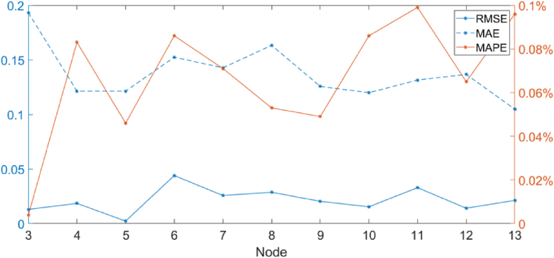
In this study, the input node is 5 and the output node is 1. Therefore, the number of nodes required to train the network is set between 3 and 13 and its error value is calculated. Figure 4 demonstrates that the error is relatively small when the number of nodes is 10. Therefore, the number of nodes in the neural network model was set to 10.

Figure 4.

Error values of different nodes.

4.1.1.2. Selection of the training function

The trainlm algorithm presents the best training effect, as shown in Table 2. Therefore, the Elman neural network model selects the trainlm algorithm as the training function.

Table 2.

Error values of different training functions.

	RMSE	MAE	MAPE
trainlm	0.0121	0.0666	0.045%
trainrp	0.0179	0.0872	0.080%
traingdx	0.0154	0.1199	0.086%

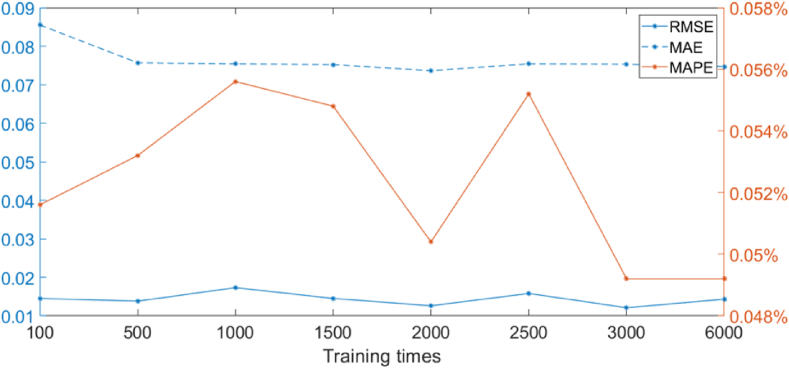
Figure 5 demonstrates that there is no significant change in the error, while the training time increases with the number of training. This article selects 300 as the number of training of the Elman neural network.

Figure 5.

Error values of different training times.

4.1.2. BP neural network modeling

The BP neural network is a multilayer feedforward network that is trained through error backpropagation. It is based on the gradient descent method, which uses the gradient search approach to minimize the mean square error between the actual and expected output value of the network. The BP algorithm involves forward propagation of the signal and backward propagation of the error. The weights and thresholds between the nodes can be adjusted and thus, the error is reduced along the gradient direction. The weights and thresholds obtained after repeated training were consistent with those of the minimum error, and the training was then stopped. The trained neural network can obtain an output value with the smallest error when compared to the actual value when receiving the input information of similar samples [19].

4.1.2.1. Selection of the BP neural network functions

The training effect of the trainlm algorithm was the best, as shown in Table 3. The root means square error, average absolute error, and average absolute percentage error obtained were the smallest when using the tansig and purelin transfer function. Therefore, the BP neural network model selects the training function as the trainlm algorithm and tansig and purelin as the transfer function.

Table 3.

Error results of different network function combinations.

Training function	Transfer function	RMSE	MAE	MAPE
trainlm	tansig purelin	0.0058	0.0314	0.0303%
	logsig tansig	0.0705	0.0937	0.0921%
	logsig purelin	0.0182	0.0843	0.13%
traingdm	tansig purelin	0.8502	12.6357	23.41%
	logsig tansig	1.0193	11.9115	21.65%
	logsig purelin	7.1208	9.5941	5.77%
trainrp	tansig purelin	0.0147	0.3690	0.16%
	logsig tansig	0.0614	1.0474	0.79%
	logsig purelin	0.0939	0.6507	0.17%

4.1.2.2. Selection of the number of nodes in the hidden layer of BP neural network

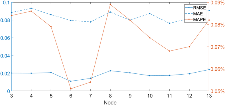
Selecting an appropriate number of hidden nodes required for high accuracy and neural network convergence requires continuous experimentation to determine the number of nodes. Figure 6 demonstrates that the error is minimum when the number of nodes is seven.

Figure 6.

Error values of different nodes.

4.1.2.3. Selection of the momentum factor and learning rate

The BP neural network reached a local minimum during training. The addition of the momentum factor at the stage can update the weight. Furthermore, an appropriate learning rate must be selected to use the BP algorithm. The smaller the learning rate, the greater the accuracy of the learning but the slower the convergence speed. The higher the learning rate, the greater the loss of information.

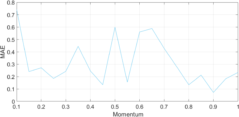
Figures 7 and 8 demonstrates that the average absolute error was the lowest when the momentum factor was 0.9 and the learning rate was 0.03. Therefore, the momentum factor of the model was set to 0.9 and the learning rate was set to 0.03.

Figure 7.

Selection of momentum factors.

Figure 8.

Selection of learning rate.

4.1.2.4. Selection of training time

The error value is small when the number of training iterations is 2000, as shown in Figure 9. Therefore, 2000 is selected as the best training time after stabilizing the number of iterations.

Figure 9.

Error values of different training times.

4.1.3. RBF neural network modeling

The RBF neural network comprises a three-layer feedforward neural network which presents good performance. The input layer receives the input variables and the hidden layer performs nonlinear conversion. Its transfer function is a radially symmetrical nonlinear attenuation function which passes to the output layer in a linear form. The output layer variable determines whether the network error meets the requirements and whether is sufficiently accurate, after which the training is stopped [20].

4.1.3.1. Selection of expansion speed, SPREAD, of the radial basis

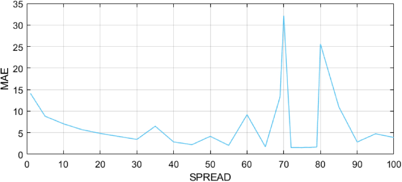
SPREAD is the expansion coefficient of the radial basis function. The larger this value, the smoother the output result. However, a large expansion coefficient can increase the calculation complexity. The expansion coefficient can be reduced appropriately if “Rank Deficient” is observed during the operation of the neural network. The average absolute error, MAE, of the 72–79 network is the smallest, and the expansion coefficient is set as 75, as shown in Figure 10.

Figure 10.

Selection of the expansion coefficient of the radial basis function.

4.1.3.2. Selection of the maximum number of neurons

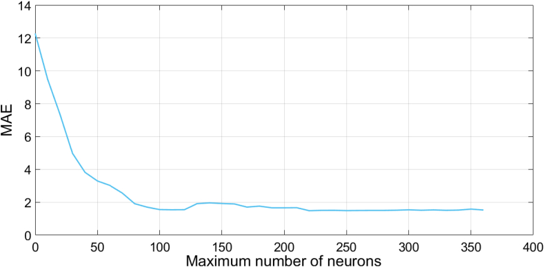
The maximum number of neurons in the hidden layer was determined when the RBF neural network is used to solve the problem. If the maximum number of neurons is too small, the resultant information processing effect is poor, and if it is too large, the calculation time is increased along with the complexity of the network structure. The neural network tends to stabilize after 248. Therefore, the maximum number of neurons is set to 248, and the average absolute error is relatively small, as shown in Figure 11.

Figure 11.

Selection of the maximum number of neurons.

4.2. Verification and comparison of simulation experimental data

The Elman neural network, BP neural network, and RBF neural network were established, and the optimal parameters were selected in the previous section. This section uses the test set for testing, and the root mean square error, mean absolute error, and mean absolute percentage error were used to compare the modeling effect presented by the three neural networks.

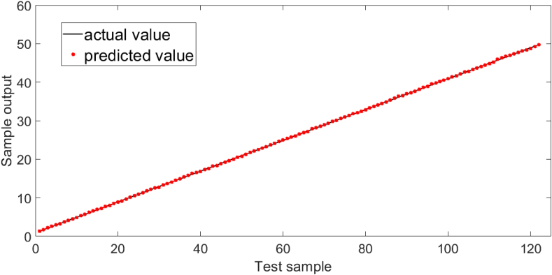
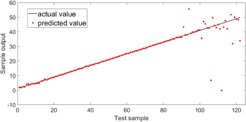
Figures 12, 13, and 14 present the prediction results of the Elman neural network, BP neural network, and RBF neural network models, respectively. Tables 4 and 5 present the comparison between the predicted and actual values of the three models along with some prediction sets. The comparison demonstrates that the prediction effect of the Elman neural network was the best.

Figure 12.

Elman neural network modeling prediction results.

Figure 13.

BP neural network modeling prediction results.

Figure 14.

RBF neural network modeling prediction results.

Table 4.

Model validation results.

	RMSE	MAE	MAPE
Elman Neural Network Modeling	0.0084	0.0637	0.045%
BP Neural Network Modeling	0.0126	0.0736	0.051%
RBF Neural Network Modeling	0.8608	1.4838	4.97%

Table 5.

Partial predicted and actual values of the channel wall.

Actual value of morphology	Elman neural network prediction	BP neural network prediction	RBF neural network prediction
1.3	1.3815	1.2663	1.9601
6.5	6.5729	6.5456	6.5057
12.1	12.2081	12.1759	12.0967
16.5	16.5692	16.5013	16.4623
21.7	21.7195	21.6783	21.6758
29.7	29.7173	29.7932	29.7924
31.3	31.2955	31.2774	31.3076
33.3	33.3583	33.3596	33.3650
36.9	36.9524	36.9093	37.3228

5. Conclusion

This study proposes a method for the inversion of the wall erosion information based on low-frequency oscillation signals and a neural network. An improved one-dimensional quasi-neutral model was developed to construct a low-frequency oscillation simulation platform. The corresponding low-frequency oscillation data were obtained by varying the cross-sectional area. A nonlinear neural network model was then established based on the obtained low-frequency oscillation data to invert the wall erosion information. The prediction results of the neural network present an adequate solution for the measurement problem. The main findings of this study can summarize as follows:

• 1.An improved one-dimensional quasi-neutral dynamic mathematical model was developed and adopted. In the simulation, the cross-sectional area is varied and disturbances are added to demonstrate that the discharge current low-frequency oscillation waveform changes under different cross-sectional areas, which provides the sample data required for neural network modeling.
• 2.Elman neural network modeling, BP neural network modeling, and RBF neural network modeling were performed for wall erosion, and the optimal parameters for the corresponding neural network were selected based on the comparison results. The Elman neural network is more stable and presents less errors, demonstrating that the Elman neural network can be used to predict the channel-wall erosion.

Declarations

Author contribution statement

Ke Han & Jie Wan: Conceived and designed the experiments; Wrote the paper.

Fang Xie & Ying Wang: Performed the experiments; Wrote the paper.

Yu Wang & Lei Zhang: Analyzed and interpreted the data; Wrote the paper.

Mengyao Yu & Jianchun Wang: Analyzed and interpreted the data.

Funding statement

Prof. Ke Han was supported by the National Natural Science Foundation of China [51736003].

Data availability statement

Data included in article/supp. material/referenced in article.

Declaration of interest's statement

The authors declare no conflict of interest.

Additional information

No additional information is available for this paper.

References

- 1.Hofer R R, Mikellides I G, Katz I and Goebel D M 2007 30th International Electric Propulsion Conference
- 2.Mao W., Wu N., Hu Y.L., Shen Y., Yao Z.P., Liu X.H. Plasma Sci. Technol. 2020;22(9):157–166. [Google Scholar]
- 3.Wei L.Q., Wei L.Q., Li W.B., Ding Y.J., Yu D.R. Plasma Sci. Technol. 2018;20(7):143–148. [Google Scholar]
- 4.Abgaryan V, Kaufman H, Kim V, 1994 30th AIAA/SAE/ASME/ASEE Joint Propulsion Conference and Exhibit, Indianapolis, Indiana, AIAA-94-2859
- 5.Baranov V, Nazarenko Y and Petrosov V 2001 27th International Electric Propulsion Conference, Pasadena, CA ,IEPC-01-48
- 6.Sommier E, Allis M, Gascon N andCappelli M 2008 42nd, 29th International Electric Propulsion Conference, Princeton, New Jersey,IEPC-2005-189
- 7.Szabo J J.2001,Fully Kinetic Numerical Modeling of a Plasma Thruster (PhD Thesis)(Boston:Massachusetts Institute of Technology)
- 8.Cho S., Komurasaki K., Arakawa YJPoP. Phys. Plasmas. 2013;20(6) [Google Scholar]
- 9.Rosenblatt FJPr. Psychol. Rev. 1958;65(6):386. doi: 10.1037/h0042519. [DOI] [PubMed] [Google Scholar]
- 10.Taccogna F., Garrigues L. Rev. Mod. Plasma Phys. 2019;3(1):1–63. [Google Scholar]
- 11.Ahedo E., Martınez-Cerezo P., Martınez-Sánchez M. Phys. Plasmas. 2001;8(6):3058–3068. [Google Scholar]
- 12.Kwon K., Walker M.L.R., Mavris D.N. Plasma Sources Sci. Technol. 2011;20(4) [Google Scholar]
- 13.Hara K, Mikellides I G 2018 2018 Joint Propulsion Conference, Cincinnati, Ohio,p4904
- 14.Morozov A.I., Savel’ev V.V. Plasma Phys. Rep. 2000;26(10):875–880. [Google Scholar]
- 15.Morozov A.I., Savel’ev V.V. Plasma Phys. Rep. 2000;26(3):219–224. [Google Scholar]
- 16.Wei L.Q., Han K., Wang C.S., Li H., Zhang C.H., Yu D.R. J. Vac. Sci. Technol.: Vacuum, Surf., Films. 2012;30(6) [Google Scholar]
- 17.Wei L.Q., Han L., Yang Z.Y., Li J., Cao Y., Yu D.R., Du J.H. J. Appl. Phys. 2015;117(5) [Google Scholar]
- 18.Zhang Z Q,Tang Z,Tang G F,Wang X G,Xiong R Q 2007 International Symposium on Neural Networks, 2007,Springer Berlin Heidelberg, Berlin
- 19.Hao Y P 2013 The 25th China Conference on Control and Decision-Making, Guiyang, China
- 20.Liu J K 2013 Radial Basis Function (RBF) Neural Network Control for Mechanical Systems. Springer, Berlin, Heidelberg
Associated Data
This section collects any data citations, data availability statements, or supplementary materials included in this article.