Moving beyond generalization to accurate interpretation of flexible models

Abstract

Machine learning optimizes flexible models to predict data. In scientific applications, there is a rising interest in interpreting these flexible models to derive hypotheses from data. However, it is unknown whether good data prediction guarantees accurate interpretation of flexible models. Here we test this connection using a flexible, yet intrinsically interpretable framework for modelling neural dynamics. We find that many models discovered during optimization predict data equally well, yet they fail to match the correct hypothesis. We develop an alternative approach that identifies models with correct interpretation by comparing model features across data samples to separate true features from noise. We illustrate our findings using recordings of spiking activity from the visual cortex of behaving monkeys. Our results reveal that good predictions cannot substitute for accurate interpretation of flexible models and offer a principled approach to identify models with correct interpretation.

Science progresses by testing theories with empirical observations. Traditionally, theories are validated with experimental data using the classical hypothesis testing paradigm¹. The hypothesis testing evaluates a statistical relationship in the data, whereby an alternative hypothesis is compared to a null hypothesis. An alternative hypothesis proposes a statistical relationship in the data, whereas a null hypothesis proposes no such relationship. Hypothesis testing is usually used for simple relationships, such as “the means are different between two data samples” (alternative hypothesis) versus “the means are the same” (null hypotheses), but elaborate relationships were also considered recently².

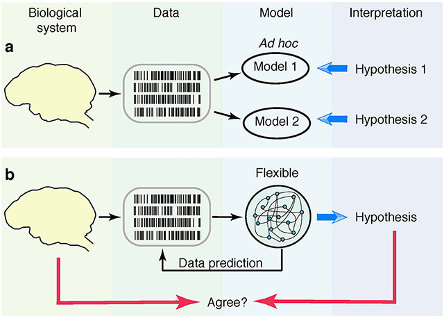
The hypothesis testing does not easily extend to many biological problems that cannot be cast into yes-no questions^3,4. In these situations, a null hypothesis is not obvious, and model selection is often used to arbitrate among several alternative hypotheses⁵. For this purpose, each alternative hypothesis is instantiated as an ad hoc mathematical model (Fig. 1a). For example, neural responses during decision-making were hypothesized to either smoothly ramp or abruptly jump on single trials, reflecting different mechanisms of evidence accumulation^6,7. These competing alternative hypotheses can be instantiated as specific mathematical models⁸. The best fitting model is then selected and used to draw conclusions about biological mechanisms^6,8–11. However, which alternative hypotheses should be considered is generally not obvious. A likely pitfall is that none of a priori guessed hypotheses may be correct⁴. This ad hoc approach, limited to a restricted hypothesis space, critically lacks flexibility.

Fig 1. Deriving theories from data.

(a) Data can be fitted with simple ad hoc models, which are based on a priori hypotheses. The hypothesis corresponding to the best fitting model is interpreted as a biological mechanism. (b) Data can be fitted with a flexible model, which covers many hypotheses within a single model architecture (typically with a large number of parameters, such as in ANNs). The model is optimized for its ability to predict new data (i.e. generalize). The hypothesis is derived by interpreting the structure of the best predictive model. It is unknown whether this approach delivers correct hypotheses that accurately reflect biological reality.

A promising alternative has emerged recently, which seeks to derive hypotheses from data using flexible models^12–15. A flexible model covers a broad class of hypotheses within a single model architecture (Fig. 1b). All hypotheses are parametrized in the same way and smooth parameter changes interpolate between hypotheses. For example, artificial neural networks (ANNs) can generate a broad spectrum of qualitatively different dynamics by adjusting weight-parameters among many interacting components in the model¹². With only loose a priori assumptions, flexible models can discover new hypotheses by fitting data, thus going beyond the classical hypotheses testing and model selection.

Flexible models enable powerful exploration of continuous hypotheses spaces, but require procedures for selecting the best parameters. Classical model selection criteria penalizing the number of parameters (e.g., various information criteria⁵) are unsuitable in this setting. Therefore, flexible models are usually optimized for their ability to predict new data (i.e. to generalize), and the best predictive model is then analysed and interpreted in terms of biological mechanisms^12–17. This widely used approach tacitly assumes that good data prediction implies correct interpretation of the model, i.e. that derived hypotheses accurately reflect physical reality. However, whether this assumption is valid is unknown. Indeed, Ptolemy’s geocentric model of the solar system predicted the movements of celestial bodies as accurately as the Copernicus’s heliocentric model. While interpreting flexible models optimized for prediction is a common practice, the derived theories can be misleading if good generalization does not guarantee correct interpretation of the model.

The link between generalization and interpretation of flexible models remained untested mainly because flexible models generally lack interpretability. Interpreting a model involves establishing the correspondence between a parameter set and the hypothesis it represents. Thus, simple ad hoc models (Fig. 1a) are interpretable by construction, as they are designed to realize one specific hypothesis with clear meaning for each parameter^8,18. In contrast, interpretation of flexible ANNs is ambiguous as it typically requires non-trivial computational steps^13,19.

To overcome this difficulty, we take advantage of a flexible, yet intrinsically interpretable modelling framework, with architecture that directly maps onto a continuous hypotheses space by design. This framework allows us to directly compare derived hypotheses with the ground truth on synthetic data. We find that selecting parameters of a flexible model by optimizing its predictions (the standard validation strategy) often produces overfitted models with spurious features not matching the ground truth. This behaviour arises because validation-based model selection relies on the classical U-shaped bias-variance trade-off, where overfitted models are expected to generalize poorly, which, however, does not always hold for flexible models with high capacity²⁰. As a result, flexible models optimized for data prediction using standard validation techniques cannot be reliably interpreted. We propose an alternative strategy for identifying models with correct interpretation by comparing model features discovered from different data samples to separate true features from noise. We apply our approach to spiking data from the primate cortex, for which the ground truth is unknown, and introduce an operational definition of correct interpretation that can be used in such cases. Counter-intuitive behaviour of flexible models with respect to generalization and model selection is at odds with conventional wisdom based on the classical bias-variance trade-off. As flexible models are gaining popularity for interpreting biological data, our results urge developing new model selection principles that prioritize accurate interpretation. We propose one such principle and demonstrate it within our modelling framework.

Results

Flexible and intrinsically interpretable framework for modelling neural dynamics.

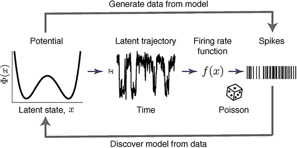
We assessed the accuracy of interpretation of flexible models by taking advantage of a flexible, yet intrinsically interpretable framework for modelling neural dynamics^21,22. This framework allows for direct comparison of the inferred hypotheses with the ground truth on synthetic data, thus testing the correctness of interpretation. Specifically, we focus on modelling dynamics of neural responses on single trials^4,6,8,9. Inference of underlying dynamical models is notoriously hard due to doubly-stochastic nature of neural spike-trains²³, leading to controversial conclusions about biological mechanisms^4,6,8,9. Spikes provide sparse and irregular sampling of noisy firing-rate trajectories on single trials, which are best described as latent dynamics²⁴. Accordingly, we model spike trains as an inhomogeneous Poisson process with time-varying intensity that depends on the latent trajectory x(t) via the firing-rate function f(x) (Fig. 2).

Fig 2. A flexible and intrinsically interpretable framework for modelling neural dynamics.

Spike data are modelled as an inhomogeneous Poisson process with intensity that depends on the latent trajectory x(t) via firing-rate function f(x). Latent dynamics are governed by a non-linear stochastic differential equation Eq. (1) with a deterministic potential Φ(x) and Gaussian noise.

In our framework, the latent dynamics are governed by a non-linear stochastic differential equation^21,22:

$$\dot{x}=-D\frac{d\mathrm{\Phi }(x)}{dx}+\sqrt{2D}\xi (t).$$ (1)

Here Φ(x) is a deterministic potential, and the noise ξ(t) with magnitude D accounts for stochasticity of latent trajectories. The potential Φ(x) can be any continuous function. Hence our framework covers a broad class of hypotheses, each represented by a non-linear dynamical system defined by Φ(x). At the same time, the shape of Φ(x) is intrinsically interpretable within dynamical systems theory, e.g., the potential minima reveal attractors²⁵. For clarity, we focus here on inference of one-dimensional Φ(x) with f(x) and D provided (our results generalize to simultaneous inference of Φ(x), f(x) and D in multiple dimensions, see Supplementary Note 1.5 and Supplementary Fig. 1).

The hypotheses are discovered from spike data Y(t) by optimizing the shape of the potential Φ(x). To efficiently search through the space of all possible Φ(x), we developed a gradient-descent optimization that maximizes the data-likelihood functional $ℒ[Y(t)\mid \mathrm{\Phi }(x)]$ (i.e. minimizes the negative log-likelihood $-\log ℒ[Y(t)\mid \mathrm{\Phi }(x)]$, see Methods). We derived analytical expression for the variational derivative of the negative log-likelihood ${\delta }_{\mathrm{\Phi }}(x)=-\delta \log ℒ[Y(t)\mid \mathrm{\Phi }(x)]/\delta \mathrm{\Phi }(x)$. Our gradient-descent algorithm increases the data likelihood by updating the potential shape: Φ(x) → Φ(x) − γδ_Φ(x) (γ is a learning-rate). Similar gradient-descent algorithms are used for optimizing ANNs²⁶.

Overfitting dynamics to stochastic spikes.

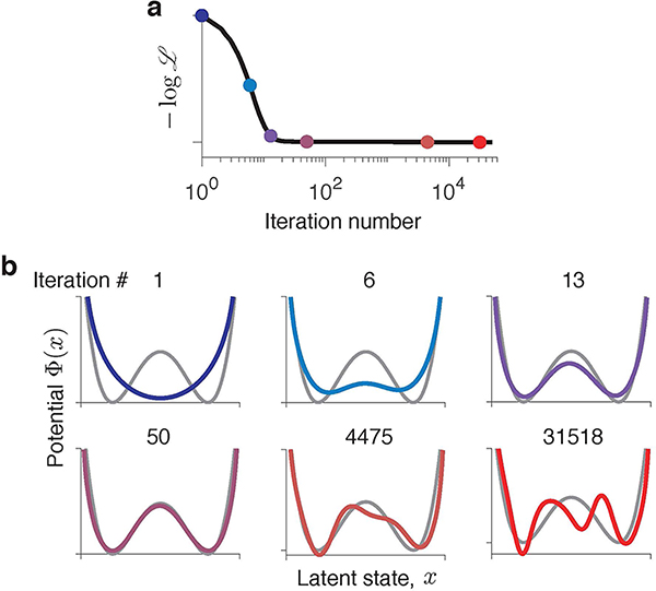
The gradient-descent optimization produces a series of dynamical models, each defined by a different potential shape Φ_n(x) (n = 1, 2, . . . is the iteration number, Fig. 3). At some intermediate iteration, the potential closely matches the ground-truth model. However, as optimization continues, Φ(x) develops spurious features not present in the ground-truth model. These spurious features arise mainly due to overfitting to the finite sample of stochastic spikes and are unique for each data sample. We verified that resampling a new data realization on each gradient-descent iteration—mimicking the infinite data regime—results in a robust recovery of the ground truth model (Extended Data Fig. 1). Overfitting to a finite spike sample is universally observed for different dynamics and data amount (Supplementary Fig. 2), which poses a challenge of selecting the correct model when the ground truth is not available.

Fig 3. Gradient descent optimization produces a series of models with different interpretations.

(a) Negative log-likelihood monotonically decreases during gradient-descent optimization. (b) Fitted potentials Φ_n(x) at selected iterations of the gradient-descent (colours correspond to dots in a) and the ground-truth potential (grey) from which the data was generated. Starting from an unspecific guess (a single-well potential on iteration 1), the optimization accurately recovers the ground-truth model (iteration 50). At later iterations, spurious features develop due to overfitting.

Generalization plateaus.

Multiple techniques exist to combat overfitting, which are all based on the idea that models matching a particular set of data too closely will fail to predict new data reliably. This guiding principle of model selection is based on the classical bias-variance trade-off²⁷. On one hand, too simple models have limited flexibility to fit the training data and hence predict new data poorly. On the other hand, too complex models fit spurious patterns in the training data resulting in poor predictions on new data. This trade-off is summarized in the classical U-shaped curve of generalization error versus model complexity, where the best generalization is achieved by models with the optimal complexity. Accordingly, the model with the best ability to generalize is selected by evaluating its performance on a validation set of data not used for training^24,27. This standard validation strategy aims at selecting models that generalize well, but whether it produces models with correct interpretation (i.e. accurately matching the ground truth) is unknown. The relationship between generalization and interpretation could possibly be non-trivial for flexible models optimized on noisy data. This relationship can be explicitly tested in our framework, which is difficult in ANNs that lack interpretability.

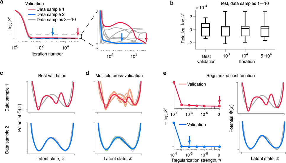
We discovered that good generalization can be achieved by many models with different interpretations. We computed the validated negative log-likelihood for each model produced by the gradient-descent using multiple samples of training and validation data generated from the same ground-truth model. The training and validated likelihoods closely track each other: after rapid initial improvement both curves level off at long plateaus (Fig. 4a, cf. Fig. 3a). Along these plateaus, we observed a continuum of models with similar likelihood but different features. Strikingly, the plateau in the validated negative log-likelihood indicates that all models along this continuum generalize almost equally well. Indeed, spurious features develop on top of the correct potential shape that is discovered first (Fig. 3b) and have little impact on the model’s ability to predict new data. For example, the overfitted models generate spike trains with the first- and second-order statistics virtually indistinguishable from the ground truth (Supplementary Fig. 3). Similar generalization plateaus are also observed in ANNs^28–30 (Extended Data Fig. 2).

Fig 4. Flexible models optimized for data prediction cannot be reliably interpreted.

(a) Validated negative log-likelihoods of models produced by the gradient-descent for ten independent samples of training and validation data generated from the same ground-truth model. Validated negative log-likelihoods exhibit long plateaus indicating a continuum of models that generalize well. A zoomed view (inset to the right) reveals the diversity of shapes of generalization plateaus. Models with the best generalization are selected at the minimum of the validated negative log-likelihood (red and blue arrows for data samples 1 and 2, respectively). (b) Relative log-likelihood with respect to the ground-truth model $\left(\left[\log ℒ-\log {ℒ}_{\text{gt}}\right]/\log {ℒ}_{\text{gt}}\right)$ evaluated on a single test data set, separate from all training and validation data, for the models at selected iterations of the gradient descent and models with the best generalization. The box-whisker plot shows the relative log-likelihood across ten samples of training and validation data. The centre line denotes the median, the box contains 25th to 75th percentiles, and the whiskers extend to the most extreme data points. (c) Models with the best generalization for data samples 1 (red) and 2 (blue) along with the ground-truth potential (grey). The model with the best generalization matches the ground truth for data sample 2 (lower panel), but exhibits spurious features for data sample 1 (upper panel). (d) Models with the best generalization selected on each fold of a nine-fold cross-validation (orange - data sample 1, teal - data sample 2), average of these models (red - data sample 1, blue - data sample 2), and the ground-truth potential (grey). The models with best generalization are correlated across folds. The average model matches the ground truth for data sample 2 (lower panel) and is overfitted for data sample 1 (upper panel). (e) Optimization of a regularized likelihood. The validated negative log-likelihoods (left panels) are shown for the models fitted with different levels of regularization η (x-axis) for data samples 1 (red) and 2 (blue). Arrows indicate the minimum of the validated negative log-likelihood, corresponding to the model with the best generalization at the optimal regularization level η^∗. The corresponding potential Φ^∗(x) (right panels, coloured lines) matches the ground truth (grey) for data sample 2 (lower panel) and is overfitted for data sample 1 (upper panel).

The observed generalization plateaus are consistent with the recent finding that the classical bias-variance trade-off does not always hold for highly flexible models²⁰. Increasing model complexity beyond a certain threshold results in improved generalisation performance. This “double-descent” curve extends the classical U-shaped bias-variance trade-off to the regime where overfitted flexible models generalize well. Our framework, like many other flexible models²⁰, operates in this regime. This idea is supported by the diversity of shapes of generalization plateaus across data samples, revealed in a zoomed view (Fig. 4a inset). The textbook U-shaped generalization curves are rare. Some generalization curves exhibit multiple local minima, some are very flat, and some still decrease at the last iteration despite the model is overfitted. This behaviour indicates that all models along the plateau generalize almost equally well and small differences in the validated likelihood arise largely from noise in the validation data. To verify this idea further, we used a single test data set, separate from all training and validation data, to evaluate log-likelihoods of models discovered at selected iterations along the plateau on different samples of training data (Fig. 4b). Across data samples, the test log-likelihoods are statistically indistinguishable among these models and the ground-truth model (one sample two-sided t-test, p = 0.98, p = 0.91 and p = 0.90 for models at iterations 10³, 10⁴ and 5 · 10⁴, respectively, n = 10), supporting the idea that all these models generalize almost equally well.

Overfitting in model selection.

The classical bias-variance trade-off suggests to control overfitting by selecting the model with the best generalization, but what does this strategy produce in the regime where many models generalize well? Following the standard validation strategy, we choose the model with the best generalization at the minimum of the validated negative log-likelihood. We found that the model with the best generalization shows little consistency across different samples of training and validation data generated from the same ground-truth model. For some data samples, the model with the best generalization closely matches the ground truth (Fig. 4c, lower panel). For other data samples, the model with the best generalization exhibits spurious features (Fig. 4c, upper row). This counter-intuitive behaviour arises because many models generalize well and the validation data, just like the training data, contain noise. As a result, any model along the generalization plateau can be chosen by chance. Note that the validation-based model selection successfully achieves its goal of finding a model with good generalization. Indeed, the log-likelihood evaluated on a test data set (separate from the training and validation data) is statistically indistinguishable between the models with the best generalization and the ground-truth model (Fig. 4b, one sample two-sided t-test, p = 0.78, n = 10). However, models with the best generalization cannot be reliably interpreted as their features do not always match the ground truth.

The problem of overfitting to noise in validation data, known as overfitting in model selection³¹, cannot be overcome with common regularization strategies. So far, we used a form of regularization called early stopping³² by selecting a model at an “early” gradient-descent iteration before reaching convergence (Fig. 4c). To mitigate noise in the validation data, early stopping is often combined with multi-fold cross-validation²⁴. This technique performs multiple rounds (folds) of training and validating the model using different partitions of the data, and the validation results are then combined (e.g., averaged) over the folds to reduce noise. However, we found that multi-fold cross-validation does not prevent overfitting in model selection (Fig. 4d). We performed nine-fold cross-validation, using 8/9 of the data for training and 1/9 for validation and rotating over the subsets used for training and validation on different folds. In this standard cross-validation scheme, the subsets of training data largely overlap between folds. Specifically, 7/8 of the training data is the same and only 1/8 is different for each pair of folds in the nine-fold cross-validation. As a result, overfitting patterns are highly correlated between folds, hence models with the best validation are also very similar across folds (Fig. 4d). Averaging these models often produces overfitted models, similar to what we observed with a single round of training and validation.

Another common regularization technique is based on modifying the optimization objective to penalize complex models²⁷. We modified the optimization objective by adding to the log-likelihood a term that discourages overly complex models:$-\ln ℒ[Y(t)\mid \mathrm{\Phi }(x)]-\eta S[\mathrm{\Phi }(x)]$. As a regularizer, we used the trajectory entropy functional S[Φ(x)], which is defined as a relative entropy between distributions of trajectories generated in the potential Φ(x) and a free diffusion³³ (see Methods). Therefore, maximizing the entropy S[Φ(x)] discourages complex trajectories. The hyperparameter η controls the balance between the data log-likelihood and regularizer: too small η does not prevent overfitting, whereas too large η results in ignoring the data and converging to the regularizer minimum. Choosing the optimal η—just like choosing the optimal iteration for early-stopping (Fig. 4a)—is usually achieved by evaluating models obtained with different η on validation data and selecting η^∗ with the best generalization²⁴. Not surprisingly, for some samples of the training and validation data, the model at η^∗ matches the ground-truth (Fig. 4e, lower row), whereas for other samples, the model at η^∗ exhibits spurious features (Fig. 4e, upper row).

Overfitting in model selection occurs for any flexible model trained and validated on finite noisy data, including ANNs (Extended Data Fig. 2). It affects any model selection procedure based on the classical bias-variance trade-off, such as maximization of Bayesian evidence, optimization of performance bounds and regularization³¹. While overfitting in model selection is less likely with more data, it is still substantial for realistic data amounts (Supplementary Table 2). As a result, flexible models optimized for their predictions cannot be reliably interpreted.

Identifying models with correct interpretation.

Our results entail that correct interpretation of flexible models requires an optimization goal different from generalization. To identify models with correct interpretation, we leverage the fact that true features are the same, whereas noise is different across data samples. Hence, comparing models discovered on different data samples could distinguish the true features from noise. The difficulty is, however, that on different data samples the same features are discovered at different iterations of the gradient-descent (Extended Data Fig. 3a). For meaningful comparisons across models, we therefore need a measure to quantify the complexity of features independent of when they are discovered. Then features of the same complexity can be directly compared to evaluate their consistency across data samples.

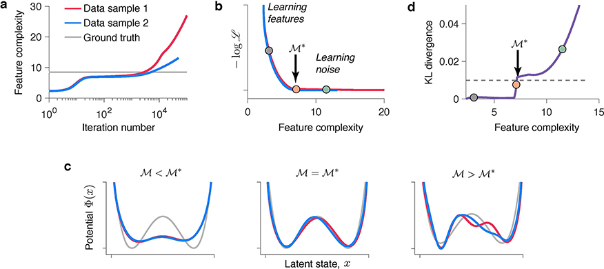
We define feature complexity as a negative entropy of latent trajectories $ℳ=-S[\mathrm{\Phi }(x)]$ (see Methods). Higher feature complexity indicates more structure in the potential Φ(x). The feature complexity increases over gradient-descent iterations, as Φ(x) develops more and more structure (Fig. 5a, similar behaviour is observed in ANNs³⁴). After the true features are discovered, $ℳ$ exceeds the ground-truth complexity, and further increases of $ℳ$ indicate fitting noise in the training data. The iteration when $ℳ$ exceeds the ground-truth complexity varies across data samples (Fig. 5a). In spite of that, the features are aligned along the complexity axis, where the boundary ${ℳ}^{*}$ separates the true features from noise (Fig. 5b). For $ℳ<{ℳ}^{*}$, the potentials of the same complexity tightly overlap between data samples (Fig. 5c, left). For $ℳ>{ℳ}^{*}$, the potentials of the same complexity diverge, since overfitting patterns are unique for each data sample (Fig. 5c, right). The potentials with complexity ${ℳ}^{*}$, where the divergence begins, match the ground-truth model (Fig. 5c, middle).

Fig 5. Identifying models with correct interpretation.

(a) Feature complexity $ℳ$ increases over the gradient-descent iterations at a rate varying across data samples. The ground-truth feature complexity is exceeded at different iterations for different data samples. (b) Normalized validated negative log-likelihood plotted against feature complexity (colours correspond to data in a). The feature complexity boundary ${ℳ}^{*}$ (orange dot) separates the true features from noise. ${ℳ}^{*}$ is the maximal feature complexity for which fitted potentials are consistent across data samples. (c) Potentials at $ℳ<{ℳ}^{*}$ (left, grey dot in b), $ℳ={ℳ}^{*}$ (middle, orange dot in b) and $ℳ>{ℳ}^{*}$ (right, teal dot in b) for data samples 1 and 2 (colours correspond to data in a). (d) KL divergence between models discovered from data samples 1 and 2 at each level of feature complexity. ${ℳ}^{*}$ is defined as the feature complexity for which the KL divergence exceeds a fixed threshold $D_{\text{KL}}^{\text{thresh}}=0.01$ (dashed line). The dots (same as in b) correspond to potentials in c.

We developed an algorithmic procedure for determining the optimal feature complexity ${ℳ}^{*}$ (see Methods). Rather than splitting the data in the usual training and validation sets, we divide the same data in two halves. We train the model on each half of the data and compare potentials with the same feature complexity discovered from the two data halves. To quantify the overlap between two potentials, we use Kullback-Leibler (KL) divergence between the corresponding equilibrium probability distributions (Fig. 5d). The KL-divergence is small for low feature complexity and then rises sharply indicating that for larger feature complexity the potentials discovered from the two data halves diverge. We define ${ℳ}^{*}$ as the feature complexity for which the KL-divergence reaches a threshold. This procedure returns two potentials corresponding to the optimal ${ℳ}^{*}$ (Fig. 5c, middle). The difference between these two potentials serves as error bars, indicating regions where the inference is less certain. The KL-threshold is a hyperparameter that sets the tolerance for mismatch between potentials. A low KL-threshold results in a conservative procedure that selects tightly overlapping potentials and can underfit complex dynamics with little data (Extended Data Fig. 5), whereas a high KL-threshold results in a liberal procedure that tolerates greater mismatch between potentials and can overfit simple dynamics. In our simulations, the KL-threshold of 0.01 produced reliable results for a broad range of ground-truth model complexities and data amounts (Supplementary Table 3).

We confirmed that our procedure reliably identifies models with correct interpretation for different ground-truth dynamics (Extended Data Figs. 3, 4, 5). Using the same amount of data, our procedure reliably identifies the correct model when generalization-based model selection often returns models with spurious features (Supplementary Note 1.7 and Supplementary Fig. 4). The generalization-based model selection tends to overfit for low-to-moderate data amounts. It can also underfit complex ground-truth dynamics for low data amount (Supplementary Table 2). In the latter regime, underfitting is expected and occurs for both methods, whereas overfitting occurs only with generalization-based and not with our feature-consistency method (Supplementary Tables 2,3). The reason for this difference is that two approaches have different objectives. Whereas validation-based model selection aims to find models that generalize well, our procedure is designed to find consistent model features in the regime where many models generalize well. Consistency of features discovered from different data samples can be used for identifying models with correct interpretation in biological data when the ground truth is unknown.

Discovering dynamics from neurophysiological recordings.

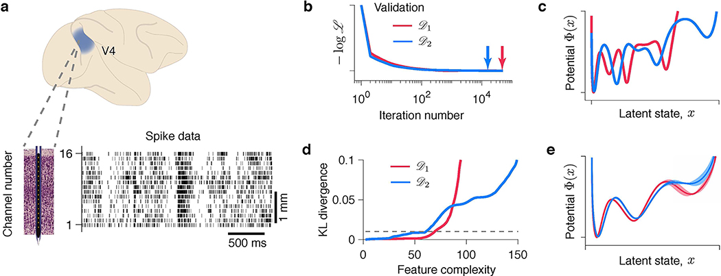
We illustrate our results using recordings of spiking activity from the visual cortex of behaving monkeys (data set from Ref.³⁵). In these data, neural activity spontaneously transitions between episodes of vigorous (On) and faint (Off) spiking that are irregular within and across trials (Fig. 6a). These endogenous On-Off dynamics were previously fitted with a model that assumes abrupt transitions between discrete On and Off states, and with an alternative model, which assumes smooth activity fluctuations³⁵. These ad hoc models with contrasting assumptions can both segment spiking activity into On and Off episodes, but they cannot resolve whether the cortical On-Off dynamics constitute fluctuations around a single attractor or transitions between multiple metastable attractors. Within our framework, these alternative hypotheses correspond to potential shapes with a single or multiple wells (Supplementary Fig. 5).

Fig 6. Discovering interpretable models of neural dynamics from neurophysiological recordings.

(a) An example trial showing spontaneous transitions between episodes of vigorous (On) and faint (Off) spiking in multiunit activity simultaneously recorded with 16-channel electrodes from the primate visual cortical area V4 during a fixation task. Spikes are marked by vertical ticks. Modelling results for an example channel are shown in b-e. (b) Validated negative log-likelihoods of models produced by the gradient-descent for two independent data samples ${𝒟}_1$ and ${𝒟}_2$. Models with the best generalization correspond to minima indicated by arrows. (c) Models with the best generalization are inconsistent across data samples (same colours as in b). (d) KL divergence between models discovered from two halves of ${𝒟}_1$ (red) and from two halves of ${𝒟}_2$ (blue) at each level of feature complexity. KL threshold (dashed line) to define ${ℳ}^{*}$ is set to 0.01. (e) The potentials at ${ℳ}^{*}$ identified independently from ${𝒟}_1$ (red) and ${𝒟}_2$ (blue) are in good agreement. Error bars shade the area between two potentials discovered from the halves of ${𝒟}_1$ (red) and ${𝒟}_2$ (blue). The potential shape supports the hypothesis of metastable transitions.

As the ground truth is not available for biological data, the most stringent test of a model selection procedure is to divide the full data set in two halves ${𝒟}_1$ and ${𝒟}_2$ and perform the optimization and model selection on each half independently. This test is strictly double-blind: optimization and model selection on ${𝒟}_1$ have no access to ${𝒟}_2$ and vice versa. An agreement between models discovered independently from ${𝒟}_1$ and ${𝒟}_2$ would indicate that the procedure reliably identifies models with the same interpretation. We therefore divide the full data set in two halves ${𝒟}_1$ and ${𝒟}_2$, and then further divide each ${𝒟}_1$ and ${𝒟}_2$ in halves: ${𝒟}_1={𝒟}_{11}\cup {𝒟}_{12}$ and ${𝒟}_2={𝒟}_{21}\cup {𝒟}_{22}$. For validation-based model selection, we perform gradient-descent optimization on ${𝒟}_{11}$ and select the model with the best validation on ${𝒟}_{12}$ (Fig. 6b,c). For the feature consistency method, we optimize models on ${𝒟}_{11}$ and ${𝒟}_{12}$ and compare features of these models to find ${ℳ}^{*}$ (Fig. 6d,e). We repeat the same steps using ${𝒟}_{21}$ and ${𝒟}_{22}$ and compare the results. We analyse spikes on each recorded channel separately (example channel in Fig. 6b–e), and then compare model fits across all channels (Extended Data Fig. 6).

With the neurophysiological recordings, we observe the same phenomena as described for synthetic data. The gradient-descent optimization continuously improves the training likelihood, producing a sequence of models with increasing feature complexity. Many of these models generalize equally well, which manifests in a long plateau in the validated negative log-likelihood (Fig. 6b). The models with the best generalization selected using the validation procedure are inconsistent between ${𝒟}_1$ and ${𝒟}_2$ (Fig. 6c), indicating likely overfitting in model selection. The disagreement between these models inferred in the double-blind test suggests that they are unlikely to faithfully capture the true system that generated both ${𝒟}_1$ and ${𝒟}_2$. In contrast, our feature consistency method identifies similar models independently on ${𝒟}_1$ and ${𝒟}_2$ for the example channel (Fig. 6e), which suggests that these models capture some of the true system’s features. The inferred potential exhibits three wells, suggesting that On-Off dynamics are metastable transitions and not fluctuations around a single attractor.

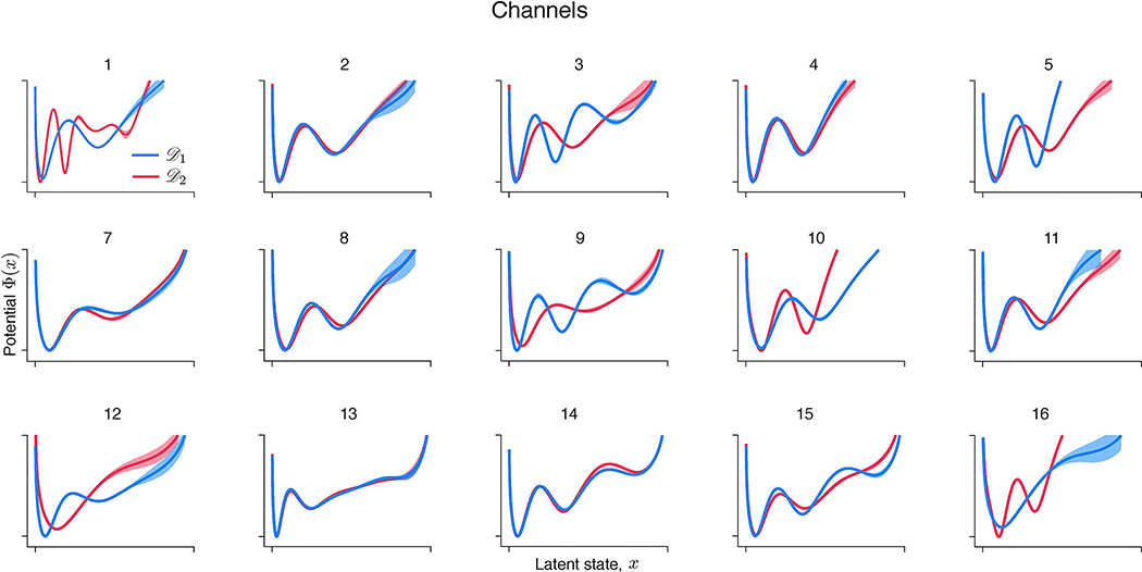
Across channels, the results are more heterogeneous, possibly due to differences in dynamics across cortical layers or underfitting on some channels (Extended Data Fig. 6). For the majority of channels (11 out of 16), the potentials discovered on ${𝒟}_1$ and ${𝒟}_2$ are in good agreement. Among these channels, some (7 out of 11) exhibit potentials with two wells and the rest exhibit three wells. For the remaining channels (5 out of 16), a potential discovered on one half of the data has fewer wells than the potential discovered on the other half. This inconsistency is a likely sign of underfitting due to insufficient data (Supplementary Note 1.7). With insufficient data, model selection is expected to favour simpler models that contain fewer features than the ground truth, which is known as Occam’s principle. Indeed, on synthetic data, our feature consistency method tends to underfit for low data amounts (Supplementary Table 3), because true features can be distorted due to insufficient sampling. In contrast, generalization-based model selection can still overfit for low data amounts (Supplementary Table 2), apparently violating Occam’s principle in the regime where overfitted models generalize well. To verify that differences across channels could arise due to underfitting, we generated synthetic data from the potential discovered by our method for the example channel (Fig. 6e). With sufficient data, our method reliably recovers this potential shape (Extended Data Fig. 5a), whereas for low data amounts, it produces underfitting patterns similar to those observed across V4 channels (Extended Data Fig. 7).

Discussion

Using a flexible and intrinsically interpretable framework, we show that flexible models optimized for data prediction cannot be reliably interpreted. Gradient-descent optimization discovers many models that generalize well despite differences in their features and interpretation. Standard model selection procedures based on the classical bias-variance trade-off yield models that generalize well but not necessarily match the correct hypothesis. Overfitting in model selection affects any flexible model fitted and validated on finite noisy data. Our results raise caution for methods based on fitting data with a flexible model and interpreting the best predictive model as a biological mechanism. Fitting flexible models requires non-trivial hyperparameter tuning geared towards models with the best generalization, and our results demonstrate that interpretation of such models is uncertain.

We introduce a principled approach for identifying models with correct interpretation by comparing features of the same complexity discovered on different data samples. Our approach differs from conventional regularization and model selection strategies routinely used with ANNs, which aim for models with the best generalization. Instead of focusing on generalization, our approach selects models based on the consistency of their features to prioritize accurate interpretation. This new approach relies on quantifying feature complexity of fitted models, which is different from conventional measures of model complexity that characterize the full capacity of the model architecture. Developing similar feature complexity measures and model selection procedures for ANNs is a significant outstanding issue, the solution of which would provide the necessary theoretical foundation for interpretable machine learning.

Our work directly tests the link between generalization and interpretation of flexible models, which have been studied only separately in ANNs that lack interpretability. In contrast to ANNs, our framework is intrinsically interpretable as it provides immediate access to fundamental dynamical features such as attractors. Interpretability is a central goal within a broader research field on automated model discovery, which aims at identification of nonlinear dynamical systems from time-series data^36–40. Within this field, we tackle the especially challenging case when both the dynamics and observations are stochastic, and therefore correctly attributing variability to the dynamics versus spiking is notoriously hard²³. Time-derivatives or time-delay embedding on which many model discovery methods rely^36–38 are not available for discrete, irregular spike trains. To uncover dynamics from stochastic spikes, we develop a gradient-descent optimization that efficiently navigates the high-dimensional space of continuous functions representing driving forces in the latent dynamical system. Other methods were proposed recently for inferring latent dynamical systems from spikes^22,41, but these studies focused exclusively on fitting methods and did not consider the problem of model selection.

Our flexible framework encompasses a broad class of hypotheses defined by general dynamical system equations. In contrast to the classical model selection, where the set of alternative hypotheses is finite and discrete, our flexible framework explores a continuous space of hypotheses, where smooth potential changes interpolate between hypotheses. Whereas the classical model selection can only produce discrete outcomes (e.g., one versus two attractors), the space of possible outcomes is far richer in our framework. The discrete outcomes are contained within this richer space as special cases, but the discovered hypothesis does not have to coincide with any of the discrete outcomes. The entire potential shape influences the interpretation. For example, deep versus shallow wells indicate relative stability of metastable attractors, and transition rates between attractors depend on the relative positions of the wells.

Our analyses of synthetic data focus on inference within the correct model class, but our framework is broadly applicable to data generated outside this model class. For example, our framework correctly infers two-well potential from spikes generated by a recurrent neural network model that exhibits bistable switching dynamics⁴² (Extended Data Fig. 8). Our framework and the spiking network model instantiate the same hypothesis on different levels of abstraction. Our framework operates on the level of population dynamics, whereas the spiking network model implements microscopic interactions among idealized neurons.

Any model involves some level of abstraction, but not every model at the same level of abstraction is accurate. For example, the On-Off dynamics in V4 could be consistent with fluctuations around a single attractor or transitions between multiple attractors. On the level of population dynamics, these alternative hypotheses correspond to potentials with single or multiple wells. The same hypotheses were also instantiated in network models with different microscopic mechanisms. For example, inhibitory stabilization can realize fluctuations around a single attractor⁴³. Short-term synaptic depression⁴⁴ or spike-rate adaption^45,46 can realize metastable transitions between two attractors with high and low firing rates. A high-dimensional recurrent network can realize multiple attractors with different firing rates⁴⁷. If the biological system is multistable, then the single-attractor hypothesis is wrong, irrespective of the underlying microscopic mechanisms. Distinguishing among these alternative hypotheses is difficult with conventional spike statistics, such as interspike interval distributions or correlations, which are similar for qualitatively different dynamics (Supplementary Fig. 3). Our framework enables the insight that cortical fluctuations reflect metastable transitions, which constraints the plausible microscopic models.

For data from complex biological systems, we propose an operational definition of correct interpretation based on an agreement between models inferred in a double-blind test. We use this operational definition to evaluate models of V4 activity (Fig. 6). Accurate statistical interpretation of the data is important for constraining detailed biophysical models, which can further reveal microscopic mechanisms generating the observed dynamics. Although latent dynamical models are widely used for interpreting biological data⁴⁸, their relation to biophysical reality is discussed less often. A promising approach for relating the statistical and biophysical descriptions is to apply the same statistical model to neural recordings and biophysical network models, to see whether the network model can reproduce the statistical structure inferred from data⁴⁹. This approach goes beyond the conventional spike statistics, such as mean rates or correlations, raising the bar for what is considered an agreement between a biophysical model and data. For example, recent studies using this strategy revealed that standard network models fail to capture the low-dimensional statistical structure observed during working memory and motor tasks^50,51, which motivated developing new network models. For this strategy to succeed, however, the statistical model is required to reliably produce correct interpretation of the data, so that the structure inferred from the data and from the correct biophysical model are expected to match, which aligns with our operational definition of correct interpretation. Our framework can therefore provide a critical link between biologically detailed models and data.

Methods

Maximum likelihood inference of latent dynamics.

Here we provide a brief summary of our methods, the full description can be found in Supplementary Notes 1 and 2. In our framework, spikes are modelled as an inhomogeneous Poisson process with time-varying intensity that depends on the latent trajectory x(t) via a non-negative firing-rate function f(x) ⩾ 0. At any moment of time, the instantaneous firing rate is f(x(t)). The latent dynamics x(t) are governed by the Langevin equation (1), where the driving force F(x) = −dΦ(x)/dx derives from the potential Φ(x), and a white Gaussian noise ξ(t) has intensity D. The spiking process is therefore controlled by two continuous functions Φ(x) and f(x), and a scalar D, which need to be inferred from data. Here we focus on inference of one-dimensional Φ(x), assuming D and f(x) are provided (see Supplementary Note 1.5 and Supplementary Fig. 1 for extensions to simultaneous inference of Φ(x), f(x) and D in multiple dimensions). All synthetic data was generated using linear f(x), and the ground-truth f(x) and D were used for the inference. For inference on the V4 data, we also use linear f(x) and fix D. Parameters for all our simulations are provided in Supplementary Note 1.6 and Supplementary Table 1.

We infer the potential Φ(x) from spike data Y (t) by maximizing the data likelihood. The likelihood functional is the probability that the data Y (t) was generated from the given model Φ(x):

$$ℒ[Y(t)\mid \mathrm{\Phi }(x)]=P(Y(t)\mid \mathrm{\Phi }(x)).$$ (2)

Here Y(t) = {t₁, t₂, …, t_N} are spike data that contain the times of all spikes. To maximize the likelihood, we iteratively minimizing the negative log-likelihood using the gradient-descent (GD) algorithm. For better numerical stability, we work with the driving force F(x) rather than potential (Supplementary Note 1.1). Thus, the GD optimization objective reads:

$$F^{*}(x)=\underset{F(x)}{\mathrm{argmin}}(-\log ℒ[Y(t)\mid F(x)]).$$ (3)

We derive analytical expressions for the log-likelihood and its variational derivative, which we evaluate numerically on each GD iteration to update the model. The potential Φ(x) is calculated from the force F(x) by taking an antiderivative (Supplementary Note 1.1).

Likelihood calculation.

Analytical derivation of the likelihood expression²¹ is briefly outlined here, see Supplementary Note 1.2 for details. The likelihood Eq. (2) is calculated via marginalization of the joint probability density $P(𝒳(t),Y(t)\mid F(x))$ of the observed spike-data Y(t) and the latent trajectory $𝒳(t)$:

$$ℒ[Y(t)\mid F(x)]=\int 𝒟𝒳(t)P(𝒳(t),Y(t)\mid F(x)).$$ (4)

Here $𝒳(t)$ represents a continuous path through the latent space, so that Eq. (4) involves a path integral. The brute-force evaluation of Eq. (4) would require intractable integration over all possible continuous latent paths $𝒳(t)$. This calculation can be simplified using the Markov property of the latent dynamics and conditional independence of observations. For the Langevin dynamics Eq. (1), the transition probability density over the latent space $p\left(x_{t_k},t_k\mid x_{t_{k-1}},t_{k-1}\right)$ does not depend on the intermediate states and can be marginalized over all paths connecting $x_{t_{k-1}}$ and $x_{t_k}$. By calculating $p\left(x_{t_k},t_k\mid x_{t_{k-1}},t_{k-1}\right)$, we can therefore effectively reduce the continuous path $𝒳(t)$ to a discrete set of points $X(t)=\left\{x_{t_0},x_{t_1},\dots ,x_{t_N}\right\}$. Since, spikes are independent when conditioned on the latent states, the joint probability density P(X(t), Y(t)) can be factorized into a product of probability densities of spike observations and transition probability densities over the latent space between the adjacent spikes:

$$P(X(t),Y(t))=p\left(x_{t_0}\right)\prod _{k=1}^{N}p\left(y_{t_i}\mid x_{t_i}\right)p\left(x_{t_i}\mid x_{t_{i-1}}\right).$$ (5)

Here Y (t) = {t₁, t₂, …, t_N} are the observed spike times and t₀ is the experiment onset time. $X(t)=\left\{x_{t_0},x_{t_1},\dots ,x_{t_N}\right\}$ is a latent trajectory at the times of spike events. $p\left(y_{t_i}\mid x_{t_i}\right)$ is the probability of observing a spike at time t_i given the latent position $x_{t_i}$. Finally, $p\left(x_{t_i}\mid x_{t_{i-1}}\right)$ is the transition probability density over the latent space from $x_{t_{i-1}}$ to $x_{t_i}$ during the time between adjacent spikes. Note that X(t) is a discretized latent path sampled at N + 1 time points. Marginalization over all intermediate time points is already performed within the transition probability densities. The likelihood is therefore calculated by marginalizing Eq. (5) over the remaining latent space variables $x_{t_i}$:

$$ℒ={\int }_{x_{t_0}}{\int }_{x_{t_1}}\dots {\int }_{x_{t_N}}d{x}_{t_0}d{x}_{t_1}\dots d{x}_{t_N}P(X(t),Y(t)).$$ (6)

The transition probability density over the latent space is a solution of the generalized Fokker-Planck equation²¹:

$$\frac{\partial p(x,t)}{\partial t}=\left(-D\frac{\partial }{\partial x}F(x)+D\frac{\partial }{\partial x^2}-f(x)\right)p(x,t)\equiv -\widehat{𝓗}p(x,t)\text{.}$$ (7)

The first two terms in the operator $\widehat{𝓗}$ are the usual drift and diffusion terms that originate from the Langevin dynamics Eq. (1). The last term −f(x) accounts for the fact that no spikes are observed during the time intervals between each pair of adjacent spikes.

The formal solution of Eq. (7) can be written as $p(x,t+\mathrm{\Delta }t)=p(x,t)\exp \{-\widehat{𝓗}\mathrm{\Delta }t\}$, where $\exp \{-\widehat{𝓗}\mathrm{\Delta }t\}$ is a linear operator that propagates probability density over the latent space. It is more convenient to work with the Hermitian version of Eq. (7) by using the transformation ρ(x, t) = p(x, t) exp(Φ(x)/2) and $𝓗=\exp (\mathrm{\Phi }(x)/2)\widehat{𝓗}\exp (-\mathrm{\Phi }(x)/2)$, where the operator $𝓗$ is Hermitian⁵². The probability density of a spike emission at a given latent state $p\left(y_{t_i}\mid x_{t_i}\right)$ is given by p(y|x) = f(x), just by the definition of the instantaneous firing rate of a Poisson process. Thus a spike emission can also be represented as a linear operator y that simply multiplies the probability density $p\left(x_{t_i}\right)$ by f(x).

Using these linear operators, we substitute Eq. (5) into Eq. (6) and rewrite the resulting likelihood expression in the Dirac’s bra-ket notation (Supplementary Note 1.2). In this notation, the probability densities ρ(x, t) are represented by state vectors ⟨ρ| upon which the linear operators act:

$$ℒ[Y(t)\mid F(x)]=\langle {\alpha }_0\left|e^{-𝓗\mathrm{\Delta }{t}_1}{\mathit{y}}_{t_1}{e}^{-𝓗\mathrm{\Delta }{t}_2}{\mathit{y}}_{t_2}\dots e^{-𝓗\mathrm{\Delta }{t}_N}{\mathit{y}}_{t_N}\right|{\beta }_{N+1}\rangle .$$ (8)

Here Δt_i = t_i −t_i−1 are interspike intervals between adjacent spikes. The bra-vector ⟨α₀| is the initial state at time t₀, and the ket vector |β_N+1⟩ accounts for the integration over $x_{t_N}$ in Eq. (6). Integrations over the intermediate variables $x_{t_i}$ (i = 0, 1, …, N − 1) are automatically realized by consecutive application of the linear operators in Eq. (8).

In computer simulations, Eq. (8) has to be represented in a discrete basis. Once discretized, the bra and ket states are represented by row and column vectors, respectively, and linear operators are represented by matrices. Thus, discretized Eq. (8) is a chain of matrix-vector products realizing the time-evolution of the bra state. The scalar likelihood results from the last dot-product in this chain between the final bra state with the ket |β_N+1⟩. Marginalizations over all intermediate latent variables $x_{t_i}$ (integrals in Eq. (6)) are therefore realized via matrix multiplications. All these calculations are most efficiently implemented in the eigenbasis of the operator $𝓗$. To find this eigenbasis, we solve the eigenvalue-eigenvector problem for the operator $𝓗$ numerically using Spectral Elements Method (SEM) (Supplementary Notes 2.1 and 2.2).

Variational derivatives of the likelihood functional.

We derive the gradient-descent algorithm for minimizing the negative log-likelihood. The gradient-descent update rule can be derived exactly, in contrast to the approximate expectation-maximization algorithm used previously²¹. This update requires to compute the variational derivative $\delta ℒ/\delta F(x)$.

The dependence of the likelihood on F(x) is hidden inside the operator $𝓗$ in Eq. (8). Using the product rule, the variational derivative can be written as:

$$\begin{array}{l}\frac{\delta ℒ}{\delta F(x)}=\sum _{\tau =0}^{N-1}\sum _{i,j}\langle {\alpha }_{\tau }\mid {\mathrm{\Psi }}_i\rangle \frac{\delta \langle {\mathrm{\Psi }}_i\left|e^{-𝓗\mathrm{\Delta }{t}_{\tau }}\right|{\mathrm{\Psi }}_j\rangle }{\delta F}\langle {\mathrm{\Psi }}_j\mid {\beta }_{\tau +1}\rangle +\\ \sum _i\frac{\delta \langle {\alpha }_0\mid {\mathrm{\Psi }}_i\rangle }{\delta F}\langle {\mathrm{\Psi }}_i\mid {\beta }_0\rangle +\langle {\alpha }_N\mid {\mathrm{\Psi }}_i\rangle \frac{\delta \langle {\mathrm{\Psi }}_i\mid {\beta }_{N+1}\rangle }{\delta F}.\end{array}$$ (9)

Here Ψ_i are the eigenvectors of $𝓗$, and ⟨α_τ|, |β_τ⟩ are the intermediate bra and ket states calculated via the forward and backward passes through the chain in Eq. (8), see Supplementary Note 1.2 for definitions.

We derived a compact expression for the variational derivative (Supplementary Note 1.3):

$$\frac{\delta ℒ}{\delta F(x)}=\sum _{ij}{G}_{ij}\frac{D}{2}{p}_{eq}(x)\frac{d\left({\varphi }_i(x){\varphi }_j(x)\right)}{dx}+{\int }_{-1}^x\left(p_{eq}(s)-\frac{{\beta }_0(s)+{\alpha }_N(s)}{2}{\rho }_{\text{eq}}(s)\right)ds.$$ (10)

Here ϕ_i(x) are scaled eigenfunctions of the operator $𝓗$, and the expression for G_ij is given in Supplementary Note 1.3.

Gradient-descent optimization.

GD algorithm updates the driving force F(x) iteratively starting from an initial guess F₀(x). We initialize optimization with F₀(x) corresponding to either a constant Φ₀(x) = −log(1/2) or a single-well Φ₀(x) = −log(cos²(πx/2)) potential (the x-domain is [−1, 1] in this work). These two potentials minimize the feature complexity for the case of Neumann and Dirichlet boundary conditions, respectively. On each iteration we calculate $ℒ$ using Eq. (8) and the variational derivative $\delta ℒ/\delta F$ using Eq. (10). The derivative of the log-likelihood is $\delta \log ℒ/\delta F=(1/ℒ)\delta ℒ/\delta F$. The force is updated as:

$$F_n(x)=F_{n-1}(x)+\gamma \frac{\delta \log ℒ}{\delta F},$$ (11)

where γ is a learning rate²⁶. The learning rate was constant over the GD iterations, but its value was different across simulations (Supplementary Table 1).

Optimization of a regularized likelihood.

In Fig. 4e, we modified the optimization objective by adding to the log-likelihood a term that discourages overly complex models:

$$-\ln ℒ[Y(t)\mid \mathrm{\Phi }(x)]-\eta S[\mathrm{\Phi }(x)],$$ (12)

where η is a hyperparameter. As a regularizer, we use the trajectory entropy functional S[Φ(x)] defined as a Kullback-Leibler divergence between the distributions $P[𝒳(t)]$ and $Q[𝒳(t)]$:

$$S[\mathrm{\Phi }(x)]=-{\int }_0^{t_{\text{obs}}}𝒟𝒳(t)P[𝒳(t)]\ln \frac{P[𝒳(t)]}{Q[𝒳(t)]}.$$ (13)

$P[𝒳(t)]$ is the probability distribution of trajectories generated from the model with the potential Φ(x). $Q[𝒳(t)]$ is the probability distribution of trajectories generated by a free diffusion (a model with a constant potential). The trajectory entropy can be expressed through the parameters of the Langevin dynamics³³ (here we only consider the terms that depend on the potential):

$$S[\mathrm{\Phi }(x)]=-\int {\left(\frac{d\mathrm{\Phi }}{dx}\right)}^2{e}^{-\mathrm{\Phi }}dx.$$ (14)

For GD optimization with the regularized cost function Eq. (12), we derived analytical expression for the variational derivative δS/δF(x) (Supplementary Note 1.4).

Feature complexity.

We define feature complexity as the negative trajectory entropy:

$$ℳ=-S[\mathrm{\Phi }(x)].$$ (15)

This measure of feature complexity is non-negative. Qualitatively, it reflects the structure of the potential Φ(x): potentials with more structure have higher feature complexity. For a particular potential Φ(x), the feature complexity is computed using Eqs. (14),(15).

Determining the optimal feature complexity.

We compare models discovered from two non-intersecting halves of the data to evaluate consistency of their features. We perform the GD optimization independently on each half of the data to obtain two series of models ${\mathrm{\Phi }}_n^1$ and ${\mathrm{\Phi }}_n^2$ (n = 1, 2 . . . is the iteration number). We measure feature complexity of all these models, ${ℳ}_n^1$ and ${ℳ}_n^2$, and quantify the overlap between potentials at the same level of feature complexity. The overlap between two potentials ${\mathrm{\Phi }}_i^1$ and ${\mathrm{\Phi }}_j^2$ is quantified using symmetrized Kullback-Leibler (KL) divergence D_KL between the corresponding equilibrium probability distributions $p_{\text{eq},i}^1$ and $p_{\text{eq},j}^2(p_{\text{eq}}(x)=\exp [-\mathrm{\Phi }(x)]$, Supplementary Note 1.1). D_KL is calculated according to:

$$D_{\text{KL}}=\int [p_{\text{eq},i}^1(x)-p_{\text{eq},j}^2(x)]\log \frac{p_{\text{eq},i}^1(x)}{p_{\text{eq},j}^2(x)}dx,$$ (16)

where the integral is evaluated numerically (Supplementary Note 2.3). Small values of D_KL indicate tight overlap between potentials, i.e. consistency of their features.

Due to noise in the data and a finite GD step-size, the GD optimization usually does not produce pairs of potentials ${\mathrm{\Phi }}_i^1$ and ${\mathrm{\Phi }}_j^2$ with the exact same feature complexity ${ℳ}_i^1={ℳ}_j^2$. Feature complexity can also slightly differ between similar potentials due to nuances of their shapes. Hence it is necessary to allow for a slack in feature complexity when comparing potentials between data samples. Accordingly, for each level of feature complexity $ℳ$, we compare all pairs of potentials ${\mathrm{\Phi }}_i^1$ and ${\mathrm{\Phi }}_j^2$ within a radius R of $ℳ$, i.e. $\left\{i:|{ℳ}_i^1-ℳ|⩽R\right\}$ and $\{j:\left|{ℳ}_j^2-ℳ\right|⩽R\}$. Among these pairs, we select the one with the minimal D_KL. This pair of most overlapping potentials and their D_KL are reported for the given $ℳ$. We repeat this procedure for a grid of $ℳ$ values along the complexity axis to produce the curve $D_{\text{KL}}(ℳ)$, such as in Fig. 5d. The optimal feature complexity ${ℳ}^{*}$ is defined as the feature complexity where this curve reaches a fixed threshold:

$${ℳ}^{*}=\underset{ℳ}{\mathrm{argmax}}{D}_{\text{KL}}(ℳ)<D_{\text{KL}}^{\text{thresh}}.$$ (17)

This procedure for determining ${ℳ}^{*}$ has two hyperparameters: the feature complexity radius R and the KL threshold $D_{\text{KL}}^{\text{thresh}}$. The radius R should be set large enough to avoid underfitting due to failure to identify similar potentials with slightly different feature complexity. Larger values of R, on the other hand, result in more pairwise model comparisons and thus increase computational time. Our procedure is otherwise not sensitive to the precise choice of R, producing the same results for any R greater than roughly 10% of the feature complexity range explored by the GD. Specifically, we use R > 1 for all synthetic data and R > 10 for V4 data. The KL threshold $D_{\text{KL}}^{\text{thresh}}$ sets the tolerance for mismatch between potentials. Choosing higher $D_{\text{KL}}^{\text{thresh}}$ results in greater discrepancy between the two selected potentials. We use $D_{\text{KL}}^{\text{thresh}}=0.01$ in all analyses (except in Extended Data Fig. 5d where we show the effect of varying $D_{\text{KL}}^{\text{thresh}}$).

Neurophysiological data.

We analysed recordings of spiking activity with 16-channel linear array electrodes from single columns of the visual area V4 in monkeys performing a fixation task. Experimental procedures and details of the dataset have been described previously³⁵. In brief, monkeys fixated on a screen for 3s to receive a juice reward. A low-contrast grating stimulus was presented on the screen in the receptive field of the recorded channels for the entire duration of fixation. We analysed activity during a sustained response to the grating stimulus (0.4 to 3s window relative to the stimulus onset).

Extended Data

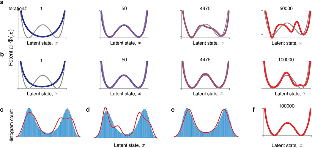
Extended Data Fig. 1. Overfitting does not occur with infinite training data.

(a) A series of models produced by the gradient-descent, when the same finite set of data is used throughout the optimization. Substantial overfitting is observed. (b) Same as a, but optimization is performed with spikes resampled on each iteration of the gradient-descent from a fixed latent trajectory (latent trajectory is the same as in a). Overfitting is still observed. (c) Histogram of the latent trajectory (normalized as probability density) and discovered equilibrium probability density (at iteration 100,000) from the simulation in b. Overfitted model contains features that are not present in the latent trajectory. (d) Same as c, but for a different latent trajectory. Spurious features in c and d are different. (e) Same as c, but with resampling both the latent trajectory and spikes on each iteration of the gradient-descent. No signs of overfitting are observed. (f) After 100,000 iterations, the inferred potential for the simulation in e still perfectly matches the ground truth. These simulations confirm that overfitting emerges largely due to Poisson noise (compare a and b), although noise in the latent trajectory also contributes to overfitting (compare b and f). No overfitting occurs when both spikes and latent trajectory are resampled on each gradient-descent iteration. In all panels, the training data contains ~10,000 spikes generated from a double-well potential.

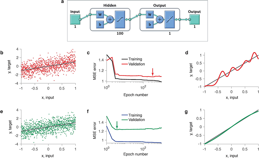
Extended Data Fig. 2. A feedforward neural network exhibits generalization plateaus and overfitting in model selection.

We trained a shallow feedforward neural network (1 hidden layer, 100 neurons, the total number of parameters is 301) on a regression problem. The noisy data set of 1,000 samples was generated from a linear model y = x + 0.2ξ, where $\xi ~𝒩(0,1)$. The network was trained using Matlab Deep Learning toolbox, which runs stochastic gradient-descent with early stopping regularization. We initialized all parameters (weights and biases) from the normal distribution with zero mean and variance 0.01. We verified that our results did not depend on a particular realization of the initial parameters. (a) Network architecture. (b) Example data set (dots) along with the linear ground-truth model (line). (c) Training and validated mean squared errors (MSEs) over the optimization epochs. Long plateau in the validated MSE indicates that many models generalize equally well. Arrow indicates the minimum of the validated MSE, i.e. the model with the best generalization. (d) The model with the best generalization (red line, corresponds to arrow in c) contains spurious features not present in the linear ground-truth model (grey line). (e) Same as b but for a different data sample from the same ground-truth model. (f) Same as c, but for the data sample in e. (g) Same as d, but for the data sample in e. The model with the best generalization (green line, corresponds to arrow in f) closely matches the ground-truth model (grey line).

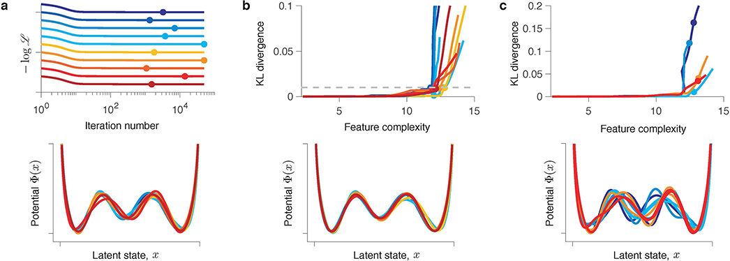
Extended Data Fig. 3. Results of model selection using the best generalization and feature consistency methods for large data amount.

Simulations are shown for ten independent data samples each with 200,000 spikes generated from the same ground-truth model (triple-well potential). Each coloured line represents one simulation. Details of the model selection procedures are provided in Supplementary Note 1.7. (a) Model selection based on the best generalization. Validated negative log-likelihood (upper panel) achieves the minimum (dots) at different gradient-descent iterations on different data samples. Fitted potentials (lower panel) selected at the minimum of the validated negative log-likelihood are consistent across data samples and with the ground-truth model for the large data amount. (b) Model selection based on feature consistency. KL divergence (upper panel) between potentials discovered from two data halves at each level of feature complexity. Models are selected at the feature complexity ${ℳ}^{*}$ (dots) where KL divergence exceeds the threshold $D_{\text{KL}}^{\text{thresh}}$ (dashed line). The selected potentials (lower panel) are consistent across data samples and with the ground-truth model. (c) Same as b, but for models selected at a larger feature complexity $ℳ>{ℳ}^{*}$ (dots). These models differ between the two data halves and are inconsistent across data samples. Only five simulations are shown for clarity.

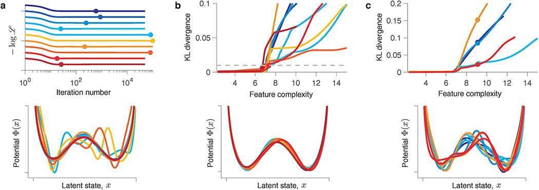
Extended Data Fig. 4. Results of model selection using the best generalization and feature consistency methods for moderate data amount.

Simulations are shown for ten independent data samples each with 20,000 spikes generated from the same ground-truth model (double-well potential). Each coloured line represents one simulation. Details of the model selection procedures are provided in Supplementary Note 1.7. (a) Model selection based on the best generalization. Validated negative log-likelihood (upper panel) achieves the minimum (dots) at different gradient-descent iterations on different data samples. Fitted potentials (lower panel) selected at the minimum of the validated negative log-likelihood are inconsistent across data samples, and many of them exhibit spurious features. (b) Model selection based on feature consistency. KL divergence (upper panel) between potentials discovered from two data halves at each level of feature complexity. Models are selected at the feature complexity ${ℳ}^{*}$ (dots) where KL divergence exceeds the threshold $D_{\text{KL}}^{\text{thresh}}$ (dashed line). The selected potentials (lower panel) are consistent across data samples and with the ground-truth model. (c) Same as b, but for models selected at a larger feature complexity $ℳ>{ℳ}^{*}$ (dots). These models differ between the two data halves and are inconsistent across data samples. Only five simulations are shown for clarity.

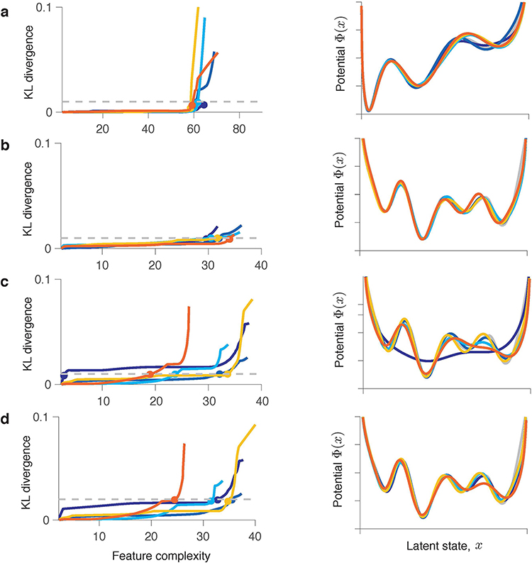
Extended Data Fig. 5. Model selection using feature consistency method for complex potential shapes.

Simulations are shown for five independent data samples generated from the same ground-truth model. Each coloured line represents one simulation. The KL-divergence (left column) between models discovered from two halves of each data sample at different levels of feature complexity. Models are selected at the feature complexity ${ℳ}^{*}$ (coloured dots) where the KL-divergence exceeds the threshold $D_{\text{KL}}^{\text{thresh}}$ (dashed line). The selected models (right column) are consistent across data samples and with the ground truth when the data amount is sufficient (a,b). Underfitting can occur for low data amounts (c,d). (a) The ground-truth is a triple-well potential with the shape inferred for the example V4 channel (Fig. 6e in the main text). Each data sample contains roughly 30,000 spikes.$D_{\text{KL}}^{\text{thresh}}=0.01$. (b) The ground-truth is a complex four-well potential. Each data sample contains roughly 400,000 spikes.$D_{\text{KL}}^{\text{thresh}}=0.01$. All five KL-curves exceed the KL-threshold. The sharp rise of KL-divergence is not yet apparent for this number of GD iterations. (c) The same ground-truth potential as in b. Each sample of synthetic data contains roughly 200,000 spikes.$D_{\text{KL}}^{\text{thresh}}=0.01$. Some of the selected models are underfitted. (d) The same data as in c but with a higher KL-threshold $D_{\text{KL}}^{\text{thresh}}=0.02$. Increasing $D_{\text{KL}}^{\text{thresh}}$ reduces underfitting of these complex dynamics resulting in more correct outcomes, but it also increases the probability of overfitting for simple ground-truth dynamics.

Extended Data Fig. 6. Discovering models of neural dynamics from neurophysiological recordings.

Potentials at ${ℳ}^{*}$ identified independently from two halves of the data, ${𝒟}_1$ (red) and ${𝒟}_2$ (blue), for other 15 channels in the recording (potentials for the example channel 6 are shown in Fig. 6e in the main text). Error bars shade the area between two potentials discovered from the halves of ${𝒟}_1$ (red) and ${𝒟}_2$ (blue). Details of this analysis are provided in the main text.

Extended Data Fig. 7. Underfitting due to small data amount for the potential shape inferred from V4 data.

We generated ten synthetic data samples from the triple-well potential with the same shape as inferred for the example V4 channel (Fig. 6e in the main text). Each sample of synthetic data contained roughly 5,000 spikes (which roughly corresponds to the amount of real data for that channel). We divided each data sample in two halves, performed gradient-descent optimization on each half, and selected the potential at ${ℳ}^{*}$ using our feature-consistency method with $D_{\text{KL}}^{\text{thresh}}=0.01$ (same as for V4 data). The selected potentials (blue) are shown along with the ground-truth (grey) in separate panels for each simulation. Error bars shade the area between potentials discovered from two data halves. Due to small data amount, underfitting is observed in roughly half of the simulations. The pattern of underfitted potential shapes across simulations resembles the pattern of potential shapes observed across V4 channels (cf. Extended Data Fig. 6).

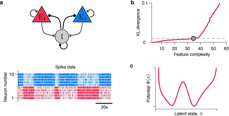
Extended Data Fig. 8. Discovering dynamics from spikes generated by microscopic simulations of a recurrent excitatory-inhibitory network model.

(a) Schematic of a recurrent balanced network model with two excitatory (E₁ and E₂) and one inhibitory (I) populations⁴². Each excitatory population consists of 400 neurons, and the inhibitory population consists of 200 neurons. The spiking neurons are simulated with the generalized integrate-and-fire (GIF) model. Details of the model architecture and simulations are described in Ref.⁴². The model exhibits winner-take-all dynamics, whereby two excitatory populations compete via the common inhibitory population. The model’s activity alternates between two attractor states, where either E₁ or E₂ has higher firing rates (lower spike raster). Spike trains of ten example neurons from E₁ (red) and E₂ (blue) are shown. This microscopic recurrent network exhibits metastable transitions between two attractors, which is the ground truth known from the theoretical analysis of the model⁴². We analysed a data set generated by microscopic simulations of this model, which contained 100 s of spiking activity of 20 neurons from the population E₁. We divided the data set in two halves, performed gradient-descent optimization on each half, and selected the potential at ${ℳ}^{*}$ using our feature-consistency method (same procedures as in all other simulations). (b) KL divergence between models discovered from two data halves at different levels of feature complexity. The model is selected at the feature complexity ${ℳ}^{*}$ (dot) where KL divergence exceeds the threshold $D_{\text{KL}}^{\text{thresh}}=0.01$ (dashed line). (c) The selected potential exhibits two attractor wells, in agreement with the ground-truth dynamics for this network model.

Data availability

All synthetic data reported in this paper can be reproduced using the source code. The synthetic and neurophysiological data are available from the corresponding author upon request.

References

- 1.Neyman J & Pearson ES On the Problem of the Most Efficient Tests of Statistical Hypotheses. Phil. Trans. R. Soc. Lond. Ser. A 231, 289–337 (1933). [Google Scholar]
- 2.Elsayed GF & Cunningham JP Structure in neural population recordings: An expected byproduct of simpler phenomena? Nat. Neurosci. 20, 1310–1318 (2017). [DOI] [PMC free article] [PubMed] [Google Scholar]
- 3.Szucs D & Ioannidis JPA When Null Hypothesis Significance Testing Is Unsuitable for Research: A Reassessment. Front. Hum. Neurosci. 11, 943–21 (2017). [DOI] [PMC free article] [PubMed] [Google Scholar]
- 4.Chandrasekaran C et al. Brittleness in model selection analysis of single neuron firing rates. BioRxiv preprint at 10.1101/430710 (2018). [DOI] [Google Scholar]
- 5.Burnham KP & Anderson DR Model Selection and Multimodel Inference: A Practical Information-Theoretic Appraoch (Springer Science & Business Media, 2007). [Google Scholar]
- 6.Bollimunta A, Totten D & Ditterich J Neural Dynamics of Choice: Single-Trial Analysis of Decision-Related Activity in Parietal Cortex. J. Neurosci. 32, 12684–12701 (2012). [DOI] [PMC free article] [PubMed] [Google Scholar]
- 7.Churchland AK et al. Variance as a Signature of Neural Computations during Decision Making. Neuron 69, 818–831 (2011). [DOI] [PMC free article] [PubMed] [Google Scholar]
- 8.Latimer KW, Yates JL, Meister ML, Huk AC & Pillow JW Single-trial spike trains in parietal cortex reveal discrete steps during decision-making. Science 349, 184–187 (2015). [DOI] [PMC free article] [PubMed] [Google Scholar]
- 9.Zoltowski DM, Latimer KW, Yates JL, Huk AC & Pillow JW Discrete stepping and nonlinear ramping dynamics underlie spiking responses of LIP neurons during decision-making. Neuron 102, 1249–1258 (2019). [DOI] [PubMed] [Google Scholar]
- 10.Durstewitz D, Koppe G & Toutounji H Computational models as statistical tools. Curr. Opin. Behav. Sci. 11, 93–99 (2016). [Google Scholar]
- 11.Linderman SW & Gershman SJ Using computational theory to constrain statistical models of neural data. Curr. Opin. Neurobiol. 46, 14–24 (2017). [DOI] [PMC free article] [PubMed] [Google Scholar]
- 12.Pandarinath C et al. Inferring single-trial neural population dynamics using sequential auto-encoders. Nat. Methods. 15, 805–815 (2018). [DOI] [PMC free article] [PubMed] [Google Scholar]
- 13.Shrikumar A, Greenside P, Shcherbina A & Kundaje A Not just a black box: Learning important features through propagating activation differences. arXiv preprint at arXiv:1605.01713 (2016). [Google Scholar]
- 14.Yamins DLK et al. Performance-optimized hierarchical models predict neural responses in higher visual cortex. Proc. Natl. Acad. Sci. 111, 8619–8624 (2014). [DOI] [PMC free article] [PubMed] [Google Scholar]
- 15.Pospisil DA & Pasupathy A ‘Artiphysiology’reveals V4-like shape tuning in a deep network trained for image classification. eLife 7, e38242 (2018). [DOI] [PMC free article] [PubMed] [Google Scholar]
- 16.Alipanahi B, Delong A, Weirauch MT & Frey BJ Predicting the sequence specificities of DNA- and RNA-binding proteins by deep learning. Nat. Biotechnol. 33, 831–838 (2015). [DOI] [PubMed] [Google Scholar]
- 17.Zhou J & Troyanskaya OG Predicting effects of noncoding variants with deep learning–based sequence model. Nat. Methods 12, 931–934 (2015). [DOI] [PMC free article] [PubMed] [Google Scholar]
- 18.Brunton BW, Botvinick MM & Brody CD Rats and humans can optimally accumulate evidence for decision-making. Science 340, 95–98 (2013). [DOI] [PubMed] [Google Scholar]
- 19.Sussillo D & Barak O Opening the black box: low-dimensional dynamics in high-dimensional recurrent neural networks. Neural Comput. 25, 626–649 (2013). [DOI] [PubMed] [Google Scholar]
- 20.Belkin M, Hsu D, Ma S & Mandal S Reconciling modern machine-learning practice and the classical bias–variance trade-off. Proc. Natl. Acad. Sci. 116, 15849–15854 (2019). [DOI] [PMC free article] [PubMed] [Google Scholar]
- 21.Haas KR, Yang H & Chu JW Expectation-Maximization of the potential of mean force and diffusion coefficient in Langevin dynamics from single molecule FRET data photon by photon. J. Phys. Chem. B 117, 15591–15605 (2013). [DOI] [PubMed] [Google Scholar]
- 22.Duncker L, Bohner G, Boussard J & Sahani M Learning interpretable continuous-time models of latent stochastic dynamical systems. arXiv preprint at arXiv:1902.04420 (2019). [Google Scholar]
- 23.Amarasingham A, Geman S & Harrison MT Ambiguity and nonidentifiability in the statistical analysis of neural codes. Proc. Natl. Acad. Sci. 112, 6455–6460 (2015). [DOI] [PMC free article] [PubMed] [Google Scholar]
- 24.Bishop CM Pattern Recognition and Machine Learning (Springer, 2006). [Google Scholar]
- 25.Yan H et al. Nonequilibrium landscape theory of neural networks. Proc. Natl. Acad. Sci. 110, E4185–94 (2013). [DOI] [PMC free article] [PubMed] [Google Scholar]
- 26.Bottou L, Curtis FE & Nocedal J Optimization Methods for Large-Scale Machine Learning. SIAM Review 60, 223–311 (2018). [Google Scholar]
- 27.Hastie T, Tibshirani R, Friedman J & Franklin J The Elements of Statistical Learning: Data Mining, Inference and Prediction (Springer, 2005). [Google Scholar]
- 28.Zhang C, Bengio S, Hardt M, Recht B & Vinyals O Understanding deep learning requires rethinking generalization. arXiv preprint at arXiv:1611.03530 (2016). [Google Scholar]
- 29.Keskar NS, Mudigere D, Nocedal J, Smelyanskiy M & Tang PTP On large-batch training for deep learning: Generalization gap and sharp minima. arXiv preprint at arXiv:1609.04836 (2016). [Google Scholar]
- 30.Ilyas A et al. Adversarial examples are not bugs, they are features. arXiv preprint at arXiv:1905.02175 (2019). [Google Scholar]
- 31.Cawley GC & Talbot NLC On over-fitting in model selection and subsequent selection bias in performance evaluation. J. Mach. Learn. Res. 11, 2079–2107 (2010). [Google Scholar]
- 32.Prechelt L Early Stopping — But When?, 53–67 (Springer Berlin Heidelberg, Berlin, Heidelberg, 2012). [Google Scholar]
- 33.Haas KR, Yang H & Chu J-W Trajectory entropy of continuous stochastic processes at equilibrium. J. Phys. Chem. Lett. 5, 999–1003 (2014). [DOI] [PubMed] [Google Scholar]
- 34.Nakkiran P et al. SGD on neural networks learns functions of increasing complexity. arXiv preprint at arXiv:1905.11604 (2019). [Google Scholar]
- 35.Engel TA et al. Selective modulation of cortical state during spatial attention. Science 354, 1140–1144 (2016). [DOI] [PubMed] [Google Scholar]
- 36.Schmidt M & Lipson H Distilling free-form natural laws from experimental data. Science 324, 81–85 (2009). [DOI] [PubMed] [Google Scholar]
- 37.Daniels BC & Nemenman I Automated adaptive inference of phenomenological dynamical models. Nat. Commun. 6, 8133–8 (2015). [DOI] [PMC free article] [PubMed] [Google Scholar]
- 38.Brunton SL, Proctor JL & Kutz JN Discovering governing equations from data by sparse identification of nonlinear dynamical systems. Proc. Natl. Acad. Sci. 113, 3932–3937 (2016). [DOI] [PMC free article] [PubMed] [Google Scholar]
- 39.Boninsegna L, Nüske F & Clementi C Sparse learning of stochastic dynamical equations. J. Chem. Phys. 148, 241723–16 (2018). [DOI] [PubMed] [Google Scholar]
- 40.Rudy SH, Nathan Kutz J & Brunton SL Deep learning of dynamics and signal-noise decomposition with time-stepping constraints. J. Comput. Phys. 396, 483–506 (2019). [Google Scholar]
- 41.Zhao Y & Park IM Variational joint filtering. arXiv preprint at arXiv:1707.09049v4 (2017). [Google Scholar]
- 42.Schwalger T, Deger M & Gerstner W Towards a theory of cortical columns: From spiking neurons to interacting neural populations of finite size. PLoS Comput. Biol. 13, e1005507–63 (2017). [DOI] [PMC free article] [PubMed] [Google Scholar]
- 43.Hennequin G, Ahmadian Y, Rubin DB, Lengyel M & Miller KD The dynamical regime of sensory cortex: Stable dynamics around a single stimulus-tuned attractor account for patterns of noise variability. Neuron 98, 846–860.e5 (2018). [DOI] [PMC free article] [PubMed] [Google Scholar]
- 44.Holcman D & Tsodyks M The emergence of Up and Down states in cortical networks. PLoS Comput. Biol. 2 (2006). [DOI] [PMC free article] [PubMed] [Google Scholar]
- 45.Jercog D et al. UP-DOWN cortical dynamics reflect state transitions in a bistable network. eLife 6, e22425 (2017). [DOI] [PMC free article] [PubMed] [Google Scholar]
- 46.Levenstein D, Buzsáki G & Rinzel J NREM sleep in the rodent neocortex and hippocampus reflects excitable dynamics. Nat. Commun. 10, 3252–12 (2019). [DOI] [PMC free article] [PubMed] [Google Scholar]
- 47.Recanatesi S, Pereira U, Murakami M, Mainen ZF & Mazzucato L Metastable attractors explain the variable timing of stable behavioral action sequences. BioRxiv preprint at 10.1101/2020.01.24.919217v1 (2020). [DOI] [PMC free article] [PubMed] [Google Scholar]
- 48.Cunningham JP & Yu BM Dimensionality reduction for large-scale neural recordings. Nat. Neurosci. 17, 1500–1509 (2014). [DOI] [PMC free article] [PubMed] [Google Scholar]
- 49.Williamson RC, Doiron B, Smith MA & Yu BM Bridging large-scale neuronal recordings and large-scale network models using dimensionality reduction. Curr. Opin. Neurobiol. 55, 40–47 (2019). [DOI] [PMC free article] [PubMed] [Google Scholar]
- 50.Murray JD et al. Stable population coding for working memory coexists with heterogeneous neural dynamics in prefrontal cortex. Proc. Natl. Acad. Sci. 114, 394–399 (2017). [DOI] [PMC free article] [PubMed] [Google Scholar]
- 51.Elsayed GF, Lara AH, Kaufman MT, Churchland MM & Cunningham JP Reorganization between preparatory and movement population responses in motor cortex. Nat. Commun. 7, 1062–15 (2016). [DOI] [PMC free article] [PubMed] [Google Scholar]
- 52.Risken H The Fokker-Planck Equation (Springer, 1996). [Google Scholar]
Associated Data
This section collects any data citations, data availability statements, or supplementary materials included in this article.
Supplementary Materials
Data Availability Statement