

Abstract
Climate change is a challenge that endangers societal TBL elements' stability. The countries' economies focus on planning for reducing carbon emissions ‘CE’ and replacing them with low CE energy. This objective needs accurate prediction for CE till 2030 via recording the most significant variables related to CE causes. The variables () are divided into two types tacking in phase I through two steps. The first step classifying the government policies that tackling by the backcasting approach to ranking them. The second step classifies the nature of the energy source which produces CE in Mega ton by SVM. The second phase is fed by phase I outputs to generate a series of prediction values by the LSTM, which is supported by the grey recruitment technique GRPT () to reduce the forecasting errors. The proposed conceptual framework named (Green Eco-Safety Monitoring; GESM), which considered a methodology gathering the backcasting, SVM, and LSTM provided by GRPT () in phase II. The paper tracks 21 governorates' CE. Proactive monitoring helps take corrective actions, enhancing the reduction in errors gap to less than 2.4%. The paper reveals that the industrial sector extracting CE at (38.67%) to 2020 with hopeful reduction of 1.72% annually if the government's interested in supporting carbon sinks, which drastically decreased to 1% by 2020 and to 0.72% annually by 2030.
Keywords: Autonomous Visual control, Cleaner production, Green indicators, Backcasting approach, Grey techniques
Highlights
-
•
Induction of reducing carbon emissions and natural resource depletion via tracking CE rate through enabling cloud technology.
-
•
Suggested conceptual framework (green eco-safety monitoring; GESM) to predict the amount of CE to 2030.
-
•
The GESM platform uses the cloud to manage a dynamic curve expressing CE's so-called visual control trend relies on grey technique.
-
•
This research presents a novel analytical approach and decision-making procedure for new town development.
Autonomous Visual control; Cleaner production; Green indicators; Backcasting approach; Grey techniques
1. Introduction
Electricity is the lifeline of civilization's progress, but it is accompanied by carbon emissions CE which have an extremely detrimental impact on human life and economic growth. The League of Arab States has a goal is to cut their imports from nations that have carbon emissions per unit of their GDP by over 65% by 2030 until their policies changed to make up 20% of primary energy consumption is non-fossil fuel i.e., renewable energy. Therefore, they call to set up projects to generate electrical power via solar, wind, etc. as a top agenda issue to serve as major hubs for replacing the use of fossil fuels like coal, Petrol, and gasoline. This study is a plan to track and predicts carbon emissions to determine the amount of investments in renewable energy economically. For the present low-carbon environmental protection programs, an accurate carbon emission ‘CE’ forecast is extremely important as suggested by Zhou et al. [1]. This concept was led by KSA in Neom City and urban new cities sprawl in Egypt. The research proposes a unique Grey Recruitment technique that discussed the new data recruitment Priority premise to increase the forecasting accuracy (i.e., self-aware). The forecast process creates a dynamic curve that expresses the trajectory of CE through what is known as a “autonomous visual control,” as a grey system theory developmental GRPT (). The Central Agency for Public Mobilization and Statistics in Egypt points to increasing the average fuel consumption to 46.5 mega tons for 12.5 mega vehicles. We are about other companies directly affecting the climate issue and dioxide emissions. In 2018, Egypt produced about 329.4 mega tons of CE ‘eq’ (GHG) emissions, according to the World Resources Institute database [2]. These values are measured in mega tons of carbon dioxide equivalent ‘eq’, representing emissions of greenhouse gases, including carbon dioxide, methane, and nitrous oxide-represented 0.6% of the global total of 49.3 billion tons of carbon dioxide ‘eq’ and nearly 10% of global emissions [3]. Egypt came in third place after Saudi Arabia and South Africa desert. Egypt's total carbon emissions increased by 140% between 1990 and 2020, with an annual average of 3.5%. During that period, Egypt's growth in total emissions was three times faster than the global average [4]. However, Egypt's GDP over the past two decades has grown faster than the growth rate of those emissions, which indicates an improvement in Egypt's carbon footprint over the past years. According to a 2018 report by the US Agency for International Development. The data showed that the energy sector produced 71.4% of carbon emissions in 2018, producing approximately 221 mega tons of [5]. The environment of electricity and heat contributes to the largest part of this %age (45%) compared to other activities in the energy sector that contribute to the rest. They are as follows: transportation (25%), manufacturing and construction (20%), the combustion of other fuels, and fugitive emissions (9%) [6], and bunker fuel (1%) [7], [8], [9]. It is worth noting that the energy sector also outperforms other sectors in the world as the largest contributor to climate change. In 2020, the use and combustion of fossil fuels – which includes coal, oil, and natural gas – emitted nearly three-quarters of greenhouse gases globally [10], [11]. Renewable energy sources accounted for only 3.4% of last year's energy mix. It is estimated that electricity produced from natural gas alone represents between 70 to 75% of the energy mix, according to 2015 World Bank data and Fitch Solutions data for 2020 [12], [13]. The country's natural gas is increasing reserves and giving the government. The priority is to generate electricity using fossil fuels to face the problem of power outages between 2011 and 2018 and as discussed by Xiang et al. [14]. Eventually, Egypt went from being short on electricity to have a surplus, but this new reality created a market that relied heavily on oil and gas. The agricultural sector was the second-largest emitter of greenhouse gases, as it produced 32 mega tons of carbon dioxide ‘eq’ or 10.2% of total emissions in 2018. Emissions from the agricultural sector increased by only 2% between 1990 and 2018. Manufacturing ranked third among the largest sectors of carbon dioxide emissions, as the total emissions from manufacturing activities and industrial processes during 2018 amounted to about 30 mega tons of carbon dioxide ‘eq’, or about 9.7% of the total emissions as understood from the analysis of Zhao et al. [15], Oda et al. [16]. The researchers settled for the density of diesel to be 0.85 kg/liter and that 1 gram of burning diesel rejects 3.16 grams of carbon dioxide and 2 grams of water, arriving at: , 2.67 kg of carbon dioxide per liter of diesel burned and of water. It assumes that about 99% of the fuel will be oxidized in a liquid hydrocarbon-burning engine. Therefore, the amount of carbon for each diesel gallon is multiplied by carbon dioxide's weight by 99%. . Each gallon of diesel fuel produces, on average, 10,084 grams of carbon dioxide, or about 22.2 pounds, as discussed by Andres et al. [17]. So, if a diesel generator uses, say, 15 gallons of diesel fuel per hour, it will produce . As a liter of gasoline weighing 0.74 kg releases 2.3 kg of carbon dioxide and 2 kg of water chemically, gasoline can be assimilated in pure octane, . There are dozens of different gasoline molecules, including additives, but they can be likened to octane. While if the density of gasoline is 0.741 kg/liter and represents a 1 gram of burning gasoline releases 3.09 grams of carbon dioxide and 2 grams of water, it amounts to: of carbon dioxide per liter of gasoline burned and of water. In short, gasoline cars, for example, if 6.0 L is consumed per 100 km, will emit 13.8 kg of CO2 for 100 km to the environment. While we find diesel engines consuming , they will reject of CO2 for 100 km is 130 g/km [3]. The CE in studied region measured by Mt unit as shown in Table 1 and the average for every country are illustrated descriptively in Fig. 1.
Table 1.
The amount of CE by Megaton in the Arab region study CEAR.
| Year | 2000 | 2001 | 2002 | 2003 | 2004 | 2005 | 2006 | 2007 | 2008 |
| CEAR | 357.8 | 364.7 | 384.05 | 415.3 | 532.41 | 823.9 | 841.7 | 856.1 | 870.8 |
| Year | 2009 | 2010 | 2011 | 2012 | 2013 | 2014 | 2015 | 2016 | 2017 |
| CEAR | 884.2 | 898.5 | 911.1 | 916.3 | 919.7 | 918.3 | 917.4 | 911.9 | 923.5 |
Figure 1.

The Arab countries emissions contribution for CE ‘Mton’.
Since the publication of the first estimate of global CE in last of 19th century, significant progress has been achieved in the development of estimating methodologies and the amount of datasets accessible. Although the availability of parallel studies should increase the accuracy and comprehension of emissions estimates, there is still a large difference between estimates and a lack of understanding of why this happens as Andrew [18].
Therefore, this article is interested in discussing a unified conceptual framework aided by KET tools and audited by the two-way of Grey methods to precisely follow the gap between the actual obtained values and the estimated ones. Although decreasing emissions in many industries may result in more upfront investment costs connected with the development of new infrastructure, the decrease in fuel use will reduce recurrent expenses. Solar panels to power a water pump in a rural community, for example, will incur a new expense at first, but the sun's energy is free. Investments in energy efficiency are also trending in the same direction [19]. As a result, these investments take on a convex form, with a cost increase over the following twenty years and a subsequent decline from previous historical levels. The impacted countries try to mitigate the consequences of climate change; additional worldwide investments of between 6 trillion and 10 trillion US dollars from the public and private sectors are required over the next decade, equating to a cumulative rate of 6 to 10% of global GDP yearly. According to IEA estimates, roughly 30% of this additional investment will come from public sources of finance on average at the worldwide level – a cumulative ratio of 2% to 3% of annual GDP during the decade from 2021 to 2030 – while the other 70% will come from private sources of funding. At the national level, the fiscal stimulus offered by governments to aid recovery from the COVID-19 epidemic is a once-in-a-lifetime chance to invest in making the transition to a global low-carbon economy. Governments should aim to shift to a more inclusive system of green budgeting as we go into the post-recovery era, examining both “brown” and “green” budget incentives and assisting budget alignment with NDCs and the Paris Agreement's climate change targets.
1.1. Just transformation
Achieving a just transformation has two primary dimensions: local and international. On the domestic side, governments need to take measures to help families who are already unable to afford necessities to pay for higher energy costs. The benefits of these measures should be communicated to coal miners, other workers, and populations whose livelihoods depend on high-carbon sectors [20]. On the international side, financial support will be necessary for developing economies, which are expected to bear high costs in the transition stage without having sufficient means to cover them.
The largest emitters, such as China, the European Union, Japan, Korea, and the United States, have pledged to bring their net emissions to zero by mid-century. This objective will not only reduce a significant proportion of global emissions. Still, it will provide technological and policy solutions to make it easier for other countries to follow this approach and make it more affordable. However, in the absence of a global climate policy, today's emitting countries will become major emitters as their populations and incomes grow. These countries are also often the countries most affected by climate change. They cannot afford the transition costs more than others due to the rapid growth of their energy needs and the dwindling of space available in their budgets to finance green investments. Previous reports are interested in creating a forecasting curve for carbon dioxide emissions and other pollutants. At the same time, in this research, the authors try to set the final expectation according to the Earth summit vision for 2030 and 2050, then use backcasting [21] to create the emission curve that is audited by the grey methods. The designed curve considers a reference for countries' policies to domesticate the tactics to achieve the desired vision. Fuel emissions are the largest cause of pollution in developing nations, especially if they utilize coke to produce electricity, which significant to GPD [22]. Therefore, establishing tools for detecting environmental violations is crucial to maintaining a stable climate. The review reveals various attempts to record significant variables that have been performed, with the majority of them focusing on regression analysis. Complete control tactics are rare, especially in the Arab Land. The back-casting technique is chosen to help in recruiting the most impacted variables to set effective policy reflect their vision toward CE reduction. This research is it's going perfectly and mimic the approach of Andrew [4] and is an extension to Le Quéré et al. [23] to include the middle east and part of north Africa in the carbon dioxide emission map as a prelude to yielding them to international control. The model's effectiveness is measured using the coefficient of determination and other statistical properties, and the results show that gathered and measured data correspond well. The simulations were run using a user-friendly software package created specifically for this purpose. The paper focuses on the emerging debate over how to use the Industry 4.0 tools such as AI, Augmented reality, Cyber physical and security systems, autonomous internet of things AIoT, and robot machines, Cloud, M2M, and Big data analysis [24], [25], [26] to change the environment need sustainable development goals [27] and Charter and Clark [28]. The peculiarity of this study is that it combines the well-known indications for maintaining a balance among the TBL elements (i.e., triple bottom line; environment, man, and economic investments [29], [30]), which are recognized as the fundamental drivers of the (CE; Circular Economy) transition. As a result, the authors want to further enhance the Local Productive Life Systems by developing a conceptual framework use back-casting to select significant variables to classify them by SVM methods pave to extract LSTM series in minimum errors [31], [32], [33]. John B. Robinson coined the term “backcasting.” Describes the fundamentals of the approach that dictate the depiction of a certain future condition in the 1980s of the previous century. It next comprises an imaginary trip backward in time, in as many steps as necessary, from the future to the present, to show how that exact future may be achieved from the present [34]. The findings show that producing energy businesses have been led and stimulated to seek sustainable environment techniques and policies by “internal variables” rather than “exterior variables” [35], [36]. The grey models described as shown in Table 2. The paper discusses the ranking of variables whether quantitative or qualitative type according to their priority to be recruited into the classification method SVM, then gathered the remaining data and creates a forecasting reference curve for the governments as discussed in Fig. 2.
Table 2.
Different grey model for prediction in brief.
| Abbrev. | Meaning of | Idiom |
|---|---|---|
| GM (1,1) | A grey model based on one variable and tackled through one first-order equation used to predict the outcome of a given situation. | x(0)(k)+az(1)(k)=b |
| DGM (1,1) | First-order equation and one variable in a discrete grey model. | x(1)(k + 1)=β1x(1)(k)+β2 |
| GRPT (1,1) | A one-variable, one-first-order equation model for predicting grey recruitment technique follow Weibull distribution. | |
| LR model | Linear regression model. | x(0)(k)=σ1k + σ2b + ε |
Figure 2.

The paper methodology plan to configure GESM.
Time series Gerami et al. [37] prediction and variable regression are two categories into which CE forecasting techniques fall. Therefore, the hybridization among LSTM expectations after classifying via SVM will lead to good results as suggested by Liu et al. [38].
2. Phase-I; Backcasting platform formulation (classification step)
This phase is interested in classifying the qualitative linguistic variables' effects on government policies to reduce the CE yearly via backcasting approach while is used the SVM in classifying the quantitative or numeric variables of CE rate to focus on significant variables only. According to Andrew [18], try to create a backcasting timely curve for studied phenomena in the Arab countries. Backcasting is a planning strategy [39], [40] that starts with establishing 2030 vision for a set of variables candidates via ridge regression (RR) and back-warded to find policies' control that will connect that optimistic future now. The authors adopted the audio signal indicator as a measure manager created to audit the damage severity through kernel function (i.e., deviation width). To improve the connection weight matrix discussed in Table 1 for the GRPT between the initial hidden layer and the output layer in the first phase, the extreme learning machine algorithm was subjected to the suggested methodology based on applying the kernel function of the SVM. Then use the grey prediction theory to forecast the significant energy consumption in the researched regions from 2000 to 2030. Variables selected from the back-casting are regressed and accurately predict CE if other factors are known in advance, and time series prediction cannot wholly utilize all CE-related data as discussed by Chen et al. [41]. According to the kind of input, the backcasting step combines the Kalman filter (KF), long short-term memory (LSTM) as cited by Graves A, Schmidhuber [42], and support vector machine (SVM) in the recruitment step to enhance the inputs election obtained from the ridge regression (RR) to regress CE values by SVM, and CE is predicted as a time series using LSTM. Consequently, based on their variances, they dubbed SVM-LSTM. The Summit on Climate Change advocated reducing CE from cars and power plants that use a lot of fuel. The authors attempt to keep track of the indicators [27] that fluctuate in relation to as expressed in Eq. (1). The influence of obtained values signals value covers a certain area ‘A; ’ for a given period ‘W; week and is inhabited by 10000 men ‘M’ through its length for numerous obtained values (N).
| (1) |
The equation (1) error is e, where 's is the contribution of the indicators, which correspond to with obtained values and may be calculated using polynomial Equation (2).
| (2) |
The reason why LSTM has increasingly supplanted GM, LSTM, etc. in time series prediction is that many traditional linear approaches are challenging to adapt to multi-input prediction situations. LSTM developed a “forget gate” to address the vanishing gradient issue for RNNs (i.e., BPNN). Today, LSTM is a potent time series prediction tool that is widely employed in the stock, energy, and economic sectors as cited by Gensler et al. [43] and Zhao et al. [44], [45]. The LSTM stages are illustrated in Fig. 3.
Figure 3.

The initial phase of LSTM integrated with the backcasting.
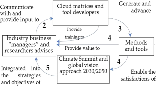
The LSTM in their initial phase based on the (the interval of study) tracked by statistically significant deviation values σs (deviation span of kernel width). The σs and k as the maximum possibility of deviation appearing. The prediction dispersal is proportional to their variance according to the kernel function, where the . () represents the priority of predecessor obtained value. The proposed GESM platform follows the backcasting technique [46], is prioritized. The proposed methodology based on type of variables affects the CE amount yearly. Therefore, suggests the next five stations as shown in Fig. 4 to tackling the qualitative variables discussed by the governments: (A) Idealistic designation for ranking based on the system's level of safety; (B) Norm defines the “as-is” state and its parameters, as well as the suggested idealistic vision, and discovers the disparity between them; (C) The amount of commitment to promoting optimal solutions and bridging gaps, and (D) Choose which imaginative connection concepts are compatible with backcasting requirements and should be implemented as routes for the vision's standard-date. (E) Using a suggested platform, handles all gathered information through autonomous internet of things ‘AIoT’ [47], [48].
Figure 4.

Overview of the conceptual framework.
2.1. The proposed GESM for an empirical action plan SVM-LSTM
The proposed methodology focuses on monitoring and predicting the CE of generating electricity via fossil fuel. The SVM-LSTM (Support Vector Machine-Long short term) model's training and test sets were derived using data on energy use CE from 2000 to 2017. When predicting, the SVM (Support Vector Machine) and LSTM models' outputs were compared with each other (Reinforcement Learning Machine). SVM-LSTM has been demonstrated to have greater accuracy. To anticipate carbon emissions in the region from 2018 to 2022 and subsequently to 2030, we lastly employed the forecasting output of AGOM (Grey Prediction Theory) () and IAGO () as the input of the SVM-LSTM model [49]. This part focuses on ensuring that the impacted variables elected from backcasting targeted the sustainability (ESS) policies [50], [51] as discussed in Fig. 4, (IS), (M) and (ES). Thus, we hypothesize:
-
:
reflect the policy correlation for the variables candidate by RR to track of ESS in their manufacturing operations.
-
:
reflect standby policy correlation of ESS variables of countries, and illustrate the vision map in Fig. 5
Figure 5.
Phase's diagram of desired vision map.
ESS: according to the policy issue (i.e., ESSM), Estimation safety variables derived from CEO interest policies established.
ESS according to the Internal variables (i.e., ESSI); Among the variables to take into account are internal variables related to the operating actions involved, features connected to internal properties, financial resource, culture, infrastructure readiness, exterior pressures, accuracy, and monitoring effectiveness [53], [61].
Variables according to Exterior effects (i.e., ESSE); Exterior variables involved legislation and regulations in the nation that yielded to the climate summit agreement.
Standby (i.e., St); Policy standby is assessed in resource efficiency by standby and resource consumption, which is tested via simplified comparable items such as those used for safety and pollution.
Current Practice (i.e., CP); Respondents the emission causes according to candidate variables from the back-casting to start classified through SVM using kernel function as illustrated in Fig. 6(a, b), while the Fig. 6(c, d) illustrates the main source for CE, which coal and diesel have maximum source for pollution.
Figure 6.

The clues of emissions causes and them relevant.
3. Phase-II: the variables classification
This phase is interested in making clusters among qualitative variables and their effects on quantitative variables to catch the tool of controlling the CE rate to precise pave to prediction which will back impact on decisions' policy. The top backcasting indicators for achieving the future vision are shown in Table 3. When backed by grey methodologies to feed the model with priority variables to be classified as discussed by SVM, then try to extract time series by the LSTM as suggested conceptual framework shown in Figure 7a, Figure 7b. The GESM sketches a reference curve tying historical obtained values each indicator with the future estimation and identifying the deviation according to the Eq. (2), taking into account the kernel function points for to create a new curve as discussed through AGO, and the IAGO method (i.e., Inverse Accumulated Generating Operation) extracts some of the predictive points that have already been transformed into AGO as cited by Li et al. [54], Li [55].
Table 3.
The back-casting establish variables and SVM suggestions (brainstorming).
| A. Safety and Sustainability variables | |||
| Plans and strategies | Measured item | Id | |
| 1. | Policy support | 1-CE rate | ESS.1 |
| 2. | Enough financial resources | 2-alternative source | ESS.2 |
| 3. | Specialization and expertise | 3-CO2 layer thickness | ESS.3 |
| 4. | Excellent infrastructure | 4-renewable projects | ESS.4 |
| 5. | You'll need an effective measuring system to keep track of the performance | 5-Cloud enabling | ESS.5 |
| 6. | Rules and regulations in the nation as well as global trends | ESS.6 | |
| B. Readiness variables | |||
| 1. | The ambition of top policy to promote long-term growth | 1-Working hours | E1 |
| 2. | Assisting with policy and strategy formulation | 2-Energy consumed | E2 |
| 3. | It is made use of specific knowledge and skill | 3-Trash disposal | E3 |
| 4. | Internal infrastructure enabling | 4-Final waste destinations | E4 |
Figure 7a.

The Proposed backcasting steps, grey controlled in an operational based on I4.0 KET for historical data collected from 2000 to 2017 [module I].
Figure 7b.

The hybridization of LSTM-SVM to verify the expected results of CE between [2018–2022] and predict under priority condition the CE from [2022–2030] module (II).
Carbon Emissions Coefficients Associated with Energy Consumption are included in the 2006 IPCC Guidelines for National Greenhouse Gas Inventories as shown in Table 4, which emphasizes that Fossil fuel combustion is the primary source of carbon emissions caused by energy use [56] and expressed in Eq. (3).
| (3) |
where represents the energy usage in tons of standard coal, represents the CE coefficient in mega tons per 109 joules, while the NCV represents the energy's low calorific content in mega J/t, and COF represents the factor for carbon oxidation. Therefore, NCV, CEC, and COF make up the coefficients of carbon emissions as discussed by Zhang et al. [57] as shown in Table 4.
Table 4.
Energy consumption CE coefficient according to their source.
| Raw coal | Petrol | Diesel | Fuel oil | Coke oven gas | Electricity | Natural gas | |
|---|---|---|---|---|---|---|---|
| Discounted coal standard kg.cm−3 | 0.7143 | 1.14714 | 1.4571 | 1.4286 | 0.5714 | 1.229 | 1.33 |
| CEC ton. trillion joule−1 | 26.8 | 18.9 | 20.2 | 21.1 | 12.1 | 10.07 t/GWh | 15.3 |
| NCV 108 J.t−1 | 209.08 | 430.7 | 426.52 | 418.16 | 173.53 | 35.96 kwh/t | 389.31 |
| COF % | 99.8 | 99.5 | 99.3 | 99.2 | 99.7 | 100 | 99.4 |
| RR P-value | ≤2.e−16 | 0.152 | 0.0154 | 0.6136 | ≤2.15.e−31 | ≤2.19.e−16 | ≤2.95.e−10 |
| PCC P-value | ≤2.19.e−16 | ≤2.1.e−9 | ≤2.1.e−8 | ≤3.86.e−42 | ≤2.15.e−31 | ≤6.68.e−62 | ≤1.54.e−25 |
a. The Eco safety variables' setup to the estimation
Despite the hundreds of cases in the design and policy literature specialized in optimizing the objective via the grey method and attempting to improve the simulation of Andrew [18], while the basic methods used grey recruitment priority estimating steps for each indicator by the GRPT () process on the doctrine Schrooten et al. [58], [61].
-
i.During period W, assemble a single indication set based on a time series as expressed in Eq. (4).
(4) -
ii.Begin by putting together the first accumulation order (differential), at , which acquire an expectable series of the AGO path, formulated as expressed in Eq. (5):
With(5) -
iii.Recruit the values of
(6) -
iv.
Following pair of v for a certain indication while , are organized for AGO for GRPT (), which identified the first differential equation in grey aspect as . If integrated to be at the interval [] [61], which discussed in Eq. (6) above.
-
v.LS guesstimate the developer coefficient φ and δ, therefore set
(8) (9) - vi.
-
vii.(IAGO) checks the approximation value of , where
(10a)
According to Mohr et al. and Ceylan [59], [60], [61], the compatibility of a government's policy norms [43]. The expected emissions via implementation the proposed technique shown in Table 5.
Table 5.
The expected CE from 2018 to 2022 based on GRPT (1,1).
| Year | ∼2018 | 2019 | 2020 | 2021 | 2022 |
|---|---|---|---|---|---|
| CE in (Mega ton) | 916.8 | 916.7 | 916.9 | 916.95 | 916.99 |
The SVM-LSTM model was then used to anticipate CE linked to energy use in the research area. We discovered the ideal model parameters after 100 tests, as shown in Table 6.
Table 6.
The SVM-LSTM model parameter set.
| Parameters | Value |
|---|---|
| The maximum number of nodes in hidden layer | 100 |
| RBF kernel parameter | 0.1 |
| Regularization coefficient C | 17 |
4. Monitoring reliability and accuracy
Check the ε% by the Eq. (11). When checking the correctness of control for each , use the Average Relative Percentage Error as expressed in Eq. (12). The accuracy standard indicators point to if ARPE is less than 10%, accurate if ARPE is between 10% and 20%, and incorrect if ARPE is greater than 50% [7] as calculated by Eq. (13). GRPT () has a precision of 92.01%, while SES's highest projected value for any indication is 86.81% as expect by Eq. (14).
| (11) |
| (12) |
| (13) |
| (14) |
The findings indicated that carbon emissions are significantly influenced by the quantity of energy consumed. We discovered that CE in the studied area can be kept below 9.59 mega tons by 2030 and that the energy consumption of electricity will be 47%. Therefore, the government's main duty in reducing the amount of carbon emissions in the following stage will be to accelerate the upgrading of the industrial structure. Selecting CE-related variables by RR comes first. Since it may successfully avoid various collinearities, RR is a standard method for choosing the most significant relevant variables to perform regression on. RR is biased since it only uses incomplete information, but the coefficients are more trustworthy. To prevent numerous collinearities and eliminate redundant information, RR is used to filter variables since we prepared 15 prospective variables that may be associated to CE and the Pearson correlation coefficients (PCC) between them and CE are all quite high with low P-values. The loss function is the primary distinction between RR and conventional linear regression. According to Eq. (15), the loss function for normal linear regression is as follows, whereas Eq. (16) as discussed in Table 5 above.
| (15) |
| (16) |
A Cronbach's alpha of 0.025, the average inter-item correlation indicates the reliability as a relation of (Backcasting outputs (ESSM, IE, EV, CP, St) + f (SVM outputs (highly energy CE sources)) [61]; a majority indicates that the data are very consistent. The countries' readiness to attain the wanted contribution has been monitored by their companies and vehicle consumption for fuel [61], [62]. The authors take the fuel consumption at different 21 governorates in Egypt that have been classified as shown in Fig. 8, CP. # 19, 8, 11, 4, 3, 21, 20, 10, 16, 9, 7, and 1 stand out in their operating system for adhering to eco-safety regulations. On the other hand, CP #18, 2, 13, 15, 6, and 5 produce a divergence. The other CPs 14, 17, and 12 may be acceptable, but they are not ideal. Fig. 9 illustrates the IoT [37] control through the AR technique; (Augmented reality) for governorate eco safety CP # 19. Table 6 depicts the obtained values deployment speed used to estimate carbon dioxide emissions during energy generation and fuel consumption at every governorate. The average values observed in participation and emission are summarized in Table 9, where Table 9 shows that ‘IS. ‘Policy’ and ‘ES.’ Take most value above the candidate variables for adopting a sustainable environment plan (), while ‘Policy’ and ‘ES.’ have the lowest value. Variables are lower in comparison () according to kernel center. Fig. 10 illustrates CE without classification or recruitment for elective data according to kernel position, while the hybridization of LSTM-SVM reduces the estimation error as illustrates in Fig. 11a if compared with native SVM or LSTM methods and with historical data only as illustrates in Fig. 11b. Table 7 shows the span series values for CE for a certain governorate over 72 weeks, where (σs in kernel width). This deviation for governorates # 19 that hopeful limit of CO2 shrinking earlier 2030. According to the findings, CE leveled out between 2000 and 2017, as seen in Fig. 12. The prediction is then verified using the actual CE forecast from 2018 to 2022 to verification stage, followed by the suggested SVM-LSTM forecast from 2020 to 2030 (Table 8). We might utilize the error covariance of training results as a rough approximation as we were unable to determine the actual error covariance of our prediction result. Soil organic carbon (SOC) and aboveground carbon (AGC) were added to obtain total ecosystem carbon stocks (TECS) as cited by Sanderman et al. [13]. This result was then multiplied by a factor of 0.48 to obtain carbon values (Kauffman and Donato [63]) according to their SOC dataset and mangrove dataset AGC as cited by Simard et al. [64]. In order to enhance CO2 sequestration and reduce future greenhouse gas emissions, the examined regions must improve their ecosystems by 0.1% year according to the prediction model. According to the SVM algorithm's basic methodology, when applied to regression fitting analysis, the goal of the algorithm is to find a classification surface that can reduce the error of all training samples from the ideal classification surface rather than to find the ideal classification surface to separate candidate samples. Carbon emission forecasting is a linearly inseparable problem due to many influencing factors. The kernel function can be used to project the sample into the high-dimensional space and simplify calculations at high latitudes. For a training candidate sample mapping via a kernel function, the sample can be mapped to a high dimensional linear space: . The issue is changed into a convex function linear programming problem by adding the relaxation factor I since the rigid constraint constraints are difficult for computers to solve as discussed in Eq. (17) and Eq. (18)
| (17) |
Quoting Lagrange factor:
| (18) |
To obtain the Lagrange dual problem, the problem is transformed into solving the equation , Eq. (19) where
| (19) |
Figure 8.

The classification of Arab countries.
Figure 9.

The visual assessment at quarter #3 of study for Co. #19 according the TBL ecosystem values.
Table 9.
The comparison indicators of the three models.
| Technique | RMSE (100%) | R2 (100%) | MRE |
|---|---|---|---|
| SVM | 40.61 | 97.97 | 6.05 |
| LSTM | 45.27 | 99.6 | 7.36 |
| SVM-LSTM | 12.34 | 99.78 | 1.63 |
Figure 10.

The recruitment impact on curve slope.
Figure 11.

The training data according to proposed technique.
Table 7.
The σs deviation for Lieq for recording and estimated data laboratory via GRPT.
| M/D | Jan | Feb | Mar | Apr | May | Jun | Jul | Aug | Sep | Oct | Nov | Dec |
|---|---|---|---|---|---|---|---|---|---|---|---|---|
| 1 | 96.30 | 97.1 | 95.4 | 128.1 | 143.0 | 156.0 | 149.1 | 149.0 | 156.0 | 151.2 | 161.0 | 161.1 |
| 2 | 96.0 | 97.0 | 99.0 | 124.0 | 134.0 | 142.0 | 151.0 | 143.1 | 155.0 | 145.1 | 163.0 | 163.0 |
| 3 | 91.0 | 90.0 | 117.0 | 94.2 | 136.0 | 141.0 | 136.1 | 154 | 141.1 | 150.2 | 139.1 | 155.0 |
| 4 | 94.0 | 92.0 | 121.0 | 95.0 | 137.1 | 142.0 | 142.0 | 153 | 142.0 | 156.1 | 157.0 | 159.0 |
| 5 | 93.0 | 91.1 | 125.0 | 100.2 | 138.0 | 150.0 | 147.1 | 156 | 150.0 | 149.0 | 160.0 | 163.1 |
| 6 | 98.0 | 122.0 | 128.1 | 130.1 | 160.0 | 160.0 | 175.0 | 185 | 190.1 | 194.0 | 197.0 | 215.1 |
Figure 12.

The results of LSTM-SVM technique based on suggested grey recruitment priority.
Table 8.
The comparing between the actual CE values and proposed prediction model, AGO, Liner regression, Long Short-Term Method, and Back Propagation Neural Network [52].
| The year | Documented values | GRPT () |
AGO () |
LR model |
LSTM |
BPNN |
|||||
|---|---|---|---|---|---|---|---|---|---|---|---|
| x(0)(k) | RPE (%) | RPE (%) | RPE (%) | RPE (%) | RPE (%) | ||||||
| 2000 | 357.8 | 445.3 | 19.65% | 449.3 | 25.57% | 452.2 | 26.38% | 467.5 | 30.66% | 601.8 | 22.73% |
| 2001 | 364.7 | 461.5 | 20.98% | 459.5 | 25.99% | 459.6 | 26.02% | 466.4 | 27.89% | 595.9 | 21.13% |
| 2002 | 384.04 | 577.7 | 33.52% | 564.7 | 47.04% | 568.5 | 48.03% | 586.8 | 52.80% | 649.6 | 23.05% |
| 2003 | 415.3 | 593.9 | 30.07% | 581.6 | 40.04% | 580.4 | 39.75% | 618.1 | 48.83% | 653.8 | 19.14% |
| 2004 | 532.41 | 540.1 | 1.42% | 560.7 | 5.31% | 562.5 | 5.65% | 545 | 2.36% | 631.9 | 6.23% |
| 2005 | 823.25 | 826.3 | 0.37% | 813.5 | 1.18% | 809.5 | 1.67% | 841.9 | 2.27% | 987 | 6.63% |
| 2006 | 841.02 | 842.5 | 0.18% | 826.5 | 1.73% | 824.1 | 2.01% | 865 | 2.85% | 964.4 | 4.89% |
| 2007 | 856.77 | 856.7 | 0.01% | 839.7 | 1.99% | 838.6 | 2.12% | 859.3 | 0.30% | 918 | 2.38% |
| 2008 | 870.05 | 870.3 | 0.03% | 853.4 | 1.91% | 853.1 | 1.95% | 887.7 | 2.03% | 1067.8 | 7.58% |
| 2009 | 884.73 | 881.7 | 0.34% | 866.7 | 2.04% | 867.7 | 1.92% | 902.8 | 2.04% | 1105.9 | 8.33% |
| 2010 | 898.96 | 897.9 | 0.12% | 880.5 | 2.05% | 882.2 | 1.86% | 922.2 | 2.59% | 1033.7 | 5.00% |
| 2011 | 911.17 | 914.1 | 0.32% | 894.5 | 1.83% | 896.8 | 1.58% | 916.4 | 0.57% | 1209 | 10.90% |
| 2012 | 916.27 | 922.7 | 0.70% | 908.8 | 0.82% | 911.4 | 0.53% | 934.7 | 2.01% | 1119.4 | 7.39% |
| 2013 | 919.71 | 921.2 | 0.16% | 923.2 | 0.38% | 925.9 | 0.67% | 929 | 1.01% | 1247.9 | 11.89% |
| 2014 | 918.67 | 920.8 | 0.23% | 937.9 | 2.09% | 940.5 | 2.38% | 939.6 | 2.28% | 1223.4 | 11.06% |
| 2015 | 917.44 | 919.5 | 0.22% | 952.9 | 3.87% | 955.1 | 4.10% | 937.7 | 2.21% | 991.7 | 2.70% |
| 2016 | 946.51 | 949.1 | 0.27% | 965.1 | 1.96% | 969.6 | 2.44% | 959.7 | 1.39% | 1147.8 | 7.09% |
| 2017 | 956.41 | 959.1 | 0.28% | 979.1 | 2.37% | 984.1 | 2.90% | 964.2 | 0.81% | 1064.9 | 3.78% |
| 2.27 | 2.22 | 2.20 | 2.4 | 1.141 | |||||||
| Validation sample | |||||||||||
| 2018 | 966.31 | 969.2 | 0.30% | 992.9 | 2.75% | 998.7 | 3.35% | 991 | 2.56% | 1211.4 | 8.45% |
| 2019 | 976.21 | 979.3 | 0.32% | 1006.9 | 3.14% | 1013.2 | 3.79% | 988.1 | 1.22% | 1247.7 | 9.27% |
| 2020 | 986.12 | 989.4 | 0.33% | 1020.8 | 3.52% | 1027.8 | 4.23% | 1008.8 | 2.30% | 1007.8 | 0.73% |
| 2021 | 996.02 | 999.5 | 0.35% | 1034.7 | 3.88% | 1042.3 | 4.65% | 1002 | 0.60% | 1242.3 | 8.24% |
| 2022 | 1005.9 | 1009.6 | 0.37% | 1048.7 | 4.25% | 1056.9 | 5.07% | 1024.9 | 1.89% | 1340.5 | 11.09% |
| 3.2 | 4.41 | 4.6 | 4.45 | 14.87 | |||||||
| 0.06 | −1.27 | −1.4 | −1.32 | −11.1 | |||||||
5. The statistical results
Table 9 shows the ideal values for the three SVM-LSTM model indicators: , , and . As demonstrated in Fig. 12 above, which summarizes the results, carbon emissions in the examined area will be gradually predicted by the model as mainly suggested by Maria et al. [12] and Abed et al. [57], [61]. While Table 10 shows the priority of variables relations between qualitative and quantitative type.
Table 10.
The weight matrix characteristics to select priority according to GPRT (1,1) data inputs for policies control the CE.
| Safety plans | ESSI | ESSE | Policy readiness | Standby Measures | |
|---|---|---|---|---|---|
| Policy ESSM | 0.7460 | ||||
| ESS-I | 0.0460 | 0.8880 | |||
| ESS-E | 0.1030 | 0.4330** | 0.7010 | ||
| Policy Readiness (E) | 0.751** | 0.0520 | 0.1780 | / | |
| Standby for Internal Variables (St-v) | -0.1670 | 0.4020** | 0.3230** | 0.0210 | 0.8651 |
| Integration of sustainability | -0.301* | 0.2561* | 0.1871 | -0.1111 | 0.420** |
For each latent variable α, the diagonal represents the Cronbach's coefficient. Other values represent the correlation weight matrix between the pairings of quantitative and qualitative variables. **, *: p-values and statistical significance were <0.01, 0.05, respectively.
As shown in Table 11, Charter and Clark advise that policy should address the following problems by concentrating less on specific areas and more on the overall framework.
Table 11.
The average policy readiness scores for the ESS variables.
| Rules | Id | Average | |
|---|---|---|---|
| A. ESS variables | |||
| Top Policy issue | ESS-M | 4.405 | |
| 1. | Senior policy responsibilities (Put your positive attention on the opportunities) | 4.1960 | |
| 2. | Supportive policy intervention (Encourage taking experience-based learning) | 4.6121 | |
| Interior resources | ESS-I | 5.0511 | |
| 3. | Enterprises targets | 5.0430 | |
| 4. | Financial resources | 5.1191 | |
| 5. | Specific expertise | 5.1171 | |
| 6. | Infrastructure developmental | 4.8741 | |
| 7. | Monitoring the performance and efficiency | 5.1031 | |
| Tackling the Exterior Variables | ESS-E | 4.5581 | |
| 8. | The bylaws in studied regions (Set up a legal foundation) | 4.2141 | |
| 9. | Socio-economic stressors | 4.3151 | |
| 10. | Exterior requirements and world trend | 5.1451 | |
| B. St. Policy | 4.3121 | ||
| 11. | Readiness of Senior policy toward a sustainable environment | S1 | 4.3121 |
| Should-be (Supporting Resource) | SS-R | 4.520 | |
| 12. | Supporting strategies set (Assign priorities) | 4.7890 | |
| 13. | financial capacity | 4.5131 | |
| 14. | Particular knowledge | 4.5460 | |
| 15. | Infrastructure construction | 4.8021 | |
| 16. | Governorate culture toward visual monitoring their environment | 4.5561 | |
| 17. | The level of sustainability environment that supports the business, comparing strategies to another environment | 3.9141 | |
| As-Is (status quo Practices) | 4.030 | ||
| 18. | Environment Resources allocation | CPx1 | 4.1031 |
5.1. Student-test
The H1 and/or H2 tested using proposed techniques according one-tailed of critical values t-test. The results of the arithmetical procedures statistically are summarized in Table 12, where the H1: , since an average over 3.56 has a favorable motivating impact (i.e., ESS implementation). The type-I error threshold of significance is .
Table 12.
The t-test results.
| The targets | Significant value | t |
Sig. | T. Value = 3.56 |
|
|---|---|---|---|---|---|
| df = 100 | Avg. (μ) | σ. | |||
| 1. ESS X Mng. | 3.34 | 09.01 | <0.001 | 4.404 | 0.86 |
| 2. ESS x Internal S variables | 3.37 | 24.98 | <0.001 | 5.0510 | 0.51 |
| 3. ESS x Exterior S variables | 3.341 | 13.120 | <0.001 | 4.558 | 0.68 |
| 4. policy Readiness | 3.231 | 05.961 | <0.001 | 4.312 | 1.140 |
| 5. supportive internal Standby measures | 3.361 | 15.171 | <0.001 | 4.520 | 0.611 |
| 6. ESS Level | 3.270 | 03.551 | 0.01 | 4.031 | 0.960 |
The primary backcasting characteristics correlation study indicates in (Table 10), where ‘Policy Readiness Culture’ results in a substantial and robust association between ‘desirable procedures’ and ‘Policy Readiness’ (0.751**). ‘IS Variables,’ ‘ES,’ and ‘Readiness’ about ‘IS’ are strongly correlated with the CE. Fig. 13 shows the best optimization tuning for monitoring CE in that impact eco safety indicators.
Figure 13.

The optimization values to control the operations to prevent the CE over allowable values.
6. Discuss
The results demonstrate that although policy preparedness is only moderately rated by generating energy businesses and environmental enterprises, they view the elements' favorable safety influence on policy's environmental, both IS and ES (Table 9 and Table 10). These activities support the claim (H1) that there is a positive correlation between policy eagerness and motivational factors (policy motivation). The information supports the second hypothesis (H2), which states that motivational traits and generating power enterprises' sustainability readiness are positively correlated. The results show that internal causes encourage internal behavior. The significant relationship between “internal supporting measures” and exterior and internal motivating factors demonstrates how motivating factors influence “internal supporting measures,” as seen in Table 10, Table 11, Table 12.
6.1. The GESM effectiveness
According to most responding countries, sustainability initiatives have a somewhat higher beneficial influence on governorate growth than other strategies toward the green vision. (: = 4.1031). Meanwhile, suggested technique fed by resources as (: = 4.11 and : = 3.91). Where, Table 9 shows the average statistical level of ESS sustainability in the governorate organization and vehicle consumption that indicates outstanding environmental performance.
Fig. 14 shows the backward of GRPT () prediction impacts to set the visual of CE value, which sketches a smooth reference path for evaluating the strategies. Also, Fig. 15 shows the which affects the obtained values. At the same time, Fig. 16 illustrates the partial success from 2000 to 2030.
Figure 14.

The predictive fluctuated points using grey LSTM method.
Figure 15.

The sound deployment at specific area for specific point appeared at Fig. 12.
Figure 16.

The prediction of most four CE sources based on the LSTM-SVM.
7. Conclusions
The proposed framework depended on two phases. The first step in the first phase uses the backcasting approach (ABCDE) to classify the qualitative variables for highlighting their impact on CE phenomena. The second step in the first phase uses the SVM to classify the quantitative variables for focusing on the high source impact of CE. The second phase presents a proactive monitoring curve built by LSTM time series based on the Grey technique GRPT () reduces the error by recruiting the important and priority variables' values. The GRPT () is a unique grey recruitment priority technique (self-aware) for fresh data during predicting the CE. The prediction generates a dynamic curve that expresses the trend of CE so-called visual control, which aims to build a Green eco-safety monitoring GESM platform managed by the cloud and considered a function of f (Backcasting, SVM, LSTM) provided by GRPT (). Therefore, called the proposed methodology SVM-LSTM because this hybridization makes direct enhancement on the predicted values as validated through the period 2000–2022. The industrial sector contributed the most to overall emissions in the first year (38.67%), followed by the construction sector (29.36%) and the transportation sector (28.20%). In the event of a redistributed scenario across all sectors, the industrial sector still accounts for the majority of carbon emissions from 2015 to 2030, with a somewhat larger percentage in the construction and industrial sectors. When compared to carbon sinks, the first year sees the removal of 1.72% of carbon emissions. The carbon sinks are drastically decreased to 1% by 2020 and to 0.72% by 2030 with the conversion of non-built regions to developed areas, proving that no program has enhanced the carbon sink. Therefore, the authors recommend cultivation of hydra trees for their reputations for absorbing CE by 1.2%. Fig. 17 guides us to focus on controlling the energy subsectors of the whole Arab governorates. Green investments are critical to the transition to a low-carbon economy and help react to the carbon price system's deployment. Investments should be increased to finance the transition from fossil fuels [65] to renewable energy sources, the adoption of intelligent electricity networks [66], energy efficiency measures, and the change to the use of electricity in different sectors such as transportation, cement industry [67], electricity generation, and construction to achieve a fundamental transformation in the current energy system. There is little question that considerable expenditures will be required throughout the transition period. Backcasting combined with the grey technique is overtly normative, entailing “traveling backward” from a certain end-point k policy measures are required to get there [68], [69]. The Grey prediction Model GRPT () is used to derive the expectations 2030–2050, as illustrated in Fig. 18. According to the examination of acquisition data, 65.8% of projects are viable. In 2000, the GESM index for the chosen regions was 52.28%, indicating that they should continue to overcome all hurdles to make good development, which hopeful reduces carbon emissions by 37% and natural resource depletion by 14% through online monitoring. For example, suppose electric vehicle charging stations are more readily available. In that case, a person looking to buy a new automobile may be more eager to buy an electric car rather than a gasoline car. Investment in research and development is also essential, and additional technological advancement will be necessary to achieve net-zero emissions.
Figure 17.

The Egyptian GHG percentage emissions.
Figure 18.

Alternative global CO2 emission pathways leading to a CO2 concentration of 400 ppm in 2100 for a reference case [5], [52], [69].
Declarations
Author contribution statement
Ahmed M. Abed, Ali AlArjani: Conceived and designed the experiments; Performed the experiments; Analyzed and interpreted the data; Contributed reagents, materials, analysis tools or data; Wrote the paper.
Funding statement
Ahmed M. Abed was supported by the Deputyship for Research & Innovation, Ministry of Education in Saudi Arabia [IF-PSAU-2022/01/22745].
Data availability statement
Data associated with this study has been deposited at https://drive.google.com/file/d/1uG_5loQCJ4HR4pF17r4jG3N_5-Rz68zo/view?usp=sharing.
Declaration of interests statement
The authors declare no conflict of interest.
Additional information
No additional information is available for this paper.
Acknowledgements
The authors extend their appreciation to the Deputyship for Research & Innovation, Ministry of Education in Saudi Arabia for funding this research work through the project number (IF-PSAU-2022/01/22745).
References
- 1.Zhou Wenhao, Zeng Bo, Wang Xiaoshuang, Luo Jianzhou, Liu Xianzhou. Forecasting Chinese carbon emissions using a novel grey rolling prediction model. Chaos Solitons Fractals. 2021;147 [Google Scholar]
- 2.https://www.iea.org/reports/co2-emissions-from-fuel-combustion-overview International Energy Agency (OECD/IEA): CO2 emissions from fuel combustion, available at.
- 3.https://www.iea.org/articles/global-co2-emissions-in-2019 International Energy Agency (OECD/IEA): global CO2 emissions in 2019, available at.
- 4.Andrew R.M. Timely estimates of India's annual and monthly fossil CO2 emissions. Earth Syst. Sci. Data. 2020;12:2411–2421. [Google Scholar]
- 5.Mabkhot M.M., Ferreira P., Maffei A., Podržaj P., Mądziel M., Antonelli D., Lanzetta M., Barata J., Boffa E., Finžgar M., et al. Mapping Industry 4.0 enabling technologies into United Nations sustainability development goals. Sustainability. 2021;13:2560. [Google Scholar]
- 6.Agora Energiewende and Sandbag The European power sector in 2018. Up-to-date analysis on the electricity transition. 2019. January 2019. https://sandbag.org.uk/project/power2018/https://sandbag.org.uk/project/ets-emissions-2018/ and update.
- 7.Crippa M., Oreggioni G., Guizzardi D., Muntean M., Schaaf E., Lo Vullo E., Solazzo E., Monforti-Ferrario F., Olivier J.G.J., Vignati E. Publications Office of the European Union; Luxembourg: 2019. Fossil CO2 emissions of all world countries.https://edgar.jrc.ec.europa.eu/overview.php?v=booklet2019 2019 Report – Study, EUR 29849 EN, JRC117610. [Google Scholar]
- 8.Crippa M., Guizzardi D., Muntean M., Schaaf E., Solazzo E., Monforti-Ferrario F., Olivier J.G.J., Vignati E. Publications Office of the European Union; Luxembourg: 2020. Fossil CO2 emissions of all world countries. 2020 Report, EUR 30358 EN, JRC121460. [Google Scholar]
- 9.Gilfillan Dennis, Marland Gregg. CDIAC-FF: global and national CO2 emissions from fossil fuel combustion and cement manufacture: 1751–2017. Earth Syst. Sci. Data. 2021;13:1667–1680. [Google Scholar]
- 10.Santoalha A., Boschma R. Diversifying in green technologies in European regions: does political support matter? Reg. Stud. 2021;55:182–195. [Google Scholar]
- 11.Olivier J.G.J., Peters J.A.H.W. PBL Netherlands Environmental Assessment Agency; The Hague: 2018. Trends in global CO2 and total GHG emissions.https://www.pbl.nl/en/publications/trends-in-global-co2-and-total-greenhouse-gasemissions-2018-report 2018 Report. [Google Scholar]
- 12.Adame Maria F., Connolly Rod M., Turschwell Mischa P., et al. Future carbon emissions from global mangrove forest loss. Glob. Change Biol. 2021;27:2856–2866. doi: 10.1111/gcb.15571. [DOI] [PMC free article] [PubMed] [Google Scholar]
- 13.Sanderman J., Hengl T., Fiske G., Solvik K., Adame M.F., Benson L., Bukoski J.J., Carnell P., Cifuentes-Jara M., Donato D., Duncan C., Eid E.M., Ermgassen P.Z., Lewis C.J.E., Macreadie P.I., Glass L., Gress S., Jardine S.L., Jones T.G., et al. A global map of mangrove forest soil carbon at 30 m spatial resolution. Environ. Res. Lett. 2018;13 [Google Scholar]
- 14.Xiang X., Cai Y., Xie S. Application of a new information priority accumulated grey model with Simpson to forecast carbon dioxide emission. J. Adv. Math. Comput. Sci. 2020;35(2):70–83. [Google Scholar]
- 15.Zhao H.R., Huang G., Yan N. Forecasting energy-related CO2 emissions employing a novel SSA-LSSVM model: considering structural factors in China. Energies. 2018;11:781. [Google Scholar]
- 16.Oda T., Maksyutov S., Andres R.J. The open-source data inventory for anthropogenic CO2, version 2018 (ODIAC2018): a global monthly fossil fuel CO2 gridded emissions data product for tracer transport simulations and surface flux inversions. Earth Syst. Sci. Data. 2020;10:87–107. doi: 10.5194/essd-10-87-2018. [DOI] [PMC free article] [PubMed] [Google Scholar]
- 17.Andres R.J., Boden T.A., Bréon F.-M., Ciais P., Davis S., Erickson D., Gregg J.S., Jacobson A., Marland G., Miller J., Oda T., Olivier J.G.J., Raupach M.R., Rayner P., Treanton K. A synthesis of carbon dioxide emissions from fossil-fuel combustion. Biogeosciences. 2012;9:1845–1871. [Google Scholar]
- 18.Andrew R.M. A comparison of estimates of global carbon dioxide emissions from fossil carbon sources. Earth Syst. Sci. Data. 2020;12:1437–1465. [Google Scholar]
- 19.EIA EIA projects U.S. energy-related CO2 emissions will remain near current level through 2050. Today Energy. 20 March 2019 [Google Scholar]
- 20.Liu Weiguo, Wang Jingxin, Bhattacharyya Debangsu, Jiang Yuan, Devallance David. Economic and environmental analyses of coal and biomass to liquid fuels. Energy. 2017;141:76–86. [Google Scholar]
- 21.Dreborg K.H. Essence of backcasting. Futures. November 1996;28(9):813–828. [Google Scholar]
- 22.Pui K.L., Othman J. The influence of economic, technical, and social aspects on energy-associated CO2 emissions in Malaysia: an extended Kaya identity approach. Energy. 2019;181:468–493. [Google Scholar]
- 23.Le Quéré C., Korsbakken J.I., Wilson C., Tosun J., Andrew R., Andres R.J., Canadell J.G., Jordan A., Peters G.P., van Vuuren D.P. Drivers of declining CO2 emissions in 18 developed economies. Nat. Clim. Change. 2019;9:213–217. [Google Scholar]
- 24.Mavropoulos A., Waage Nilsen A. John Wiley and Sons; Chichester, UK: 2020. Industry 4.0 and Circular Economy: Towards a Wasteless Future or a Wasteful Planet? [Google Scholar]
- 25.Ramirez P. In: Industry 4.0 and Regional Transformations. De Propris L., Bailey D., editors. Routledge; London, UK: 2020. Sustainable production: creating a regional forest-based bio-economy; pp. 97–111. [Google Scholar]
- 26.Zhijun P., Bo P., Weiguo H., Jianzhong S., Bangpeng X., Wenkai Z., Jialin W., Xiaopeng L., Jing G., Yang W., et al. Energy monitoring method based on big data intelligent analysis technology and energy cloud platform. 16 August 2019. https://worldwide.espacenet.com/patent/search/family/067583244/publication/CN110138877A?q=pn%3DCN110138877A Patent CN 110138877A, Available online.
- 27.Hermans F.L.P. In: Rethinking Clusters: Place-Based Value Creation in Sustainability Transitions. Sedita S.R., Blasi S., editors. Springer Nature Switzerland AG; Cham, Switzerland: 2021. Bioclusters and sustainable regional development; pp. 81–91. [Google Scholar]
- 28.Charter M., Clark T. Sustainable Innovation, 2003–2006. University College for the Creative Arts; Farnham, UK: 2007. Sustainable innovation: key conclusions from sustainable innovation conferences 2003–2006 organised by the Centre for Sustainable Design. [Google Scholar]
- 29.Cai Y., Etzkowitz H. Theorizing the Triple Helix model: past, present, and future. Triple Helix. 2020;7:189–226. [Google Scholar]
- 30.Le Moigne R. The power of digital technologies to enable the circular economy. 2021. https://medium.com/circulatenews/the-power-of-digital-technologies-to-enable-the-circular-economy-5471d097ee7f Available online.
- 31.Bellandi M., Plechero M., Santini E. Forms of place leadership in local productive systems: from endogenous rerouting to deliberate resistance to change. Reg. Stud. 2021;55:1327–1336. [Google Scholar]
- 32.Sandborn Peter, Lucyshyn William. Handbook of Advanced Performability Engineering. 2021. Sustainment strategies for system performance enhancement; pp. 271–297. [Google Scholar]
- 33.Satyro W.C., Contador J.C., Contador J.L., Fragomeni M.A., Monken S.F.d.P., Ribeiro A.F., de Lima A.F., Gomes J.A., do Nascimento J.R., de Araújo J.L., et al. Implementing Industry 4.0 through cleaner production and social stakeholders: holistic and sustainable model. Sustainability. 2021;13:12479. [Google Scholar]
- 34.Robinson J.B. Unlearning and backcasting: rethinking some of the questions we ask about the future. Technol. Forecast. Soc. Change. July 1988;33(4):325–338. [Google Scholar]
- 35.Hoppe T., Miedema M.A. Governance approach to regional energy transition: meaning, conceptualization and practice. Sustainability. 2020;12:915. [Google Scholar]
- 36.Kant Nikhil. Industry, Innovation and Infrastructure. 2020. Climate strategy proactivity (CSP) and its theoretical underpinnings; pp. 1–13. [Google Scholar]
- 37.Gerami M.H., Rabbaniha M. Forecasting the anchovy kilka fishery in the Caspian Sea using a time series approach. Turk. J. Fish. Aquat. Sci. 2018;18:1288–1292. [Google Scholar]
- 38.Liu H., Mi X.W., Li Y.F. An experimental investigation of three new hybrid wind speed forecasting models using multi-decomposing strategy and ELM algorithm. Renew. Energy. 2018;123:694–705. [Google Scholar]
- 39.Bailey D., Pitelis C., Tomlinson P. Strategic policy and regional industrial strategy: cross-fertilization to mutual advantage. Reg. Stud. 2020;54:647–659. [Google Scholar]
- 40.Han P., Zeng N., Oda T., Lin X., Crippa M., Guan D., Janssens-Maenhout G., Ma X., Liu Z., Shan Y., Tao S., Wang H., Wang R., Wu L., Yun X., Zhang Q., Zhao F., Zheng B. Evaluating China's fossil-fuel CO2 emissions from a comprehensive dataset of nine inventories. Atmos. Chem. Phys. 2020;20:11371–11385. [Google Scholar]
- 41.Chen K., Zhou Y., Dai F. A LSTM-based method for stock returns prediction: a case study of China stock market. 2015 IEEE International Conference on Big Data; Big Data; IEEE; 2015. pp. 2823–2824. [Google Scholar]
- 42.Graves A., Schmidhuber J. Framewise phoneme classification with bidirectional LSTM and other neural network architectures. Neural Netw. 2005;2005(18):602–610. doi: 10.1016/j.neunet.2005.06.042. [DOI] [PubMed] [Google Scholar]
- 43.Gensler A., Henze J., Sick B., Raabe N. Deep learning for solar power forecasting—an approach using auto encoder and LSTM neural networks. 2016 IEEE International Conference on Systems, Man, and Cybernetics; SMC; IEEE; 2016. pp. 2858–2865. [Google Scholar]
- 44.Zhao Z.D., Hu C.Z. Grey prediction models for the standard limit of vehicle noise. Proc. Inst. Mech. Eng., Part D, J. Automob. Eng. 2018;2018(232):973–979. [Google Scholar]
- 45.Zhao T., Hu Y., Zang T., Cheng L. Identifying Alzheimer's disease-related proteins by LRRGD. BMC Bioinform. 2019;2019(20):570. doi: 10.1186/s12859-019-3124-7. [DOI] [PMC free article] [PubMed] [Google Scholar]
- 46.Alberti F.G., Belfanti F. In: Rethinking Clusters: Place-Based Value Creation in Sustainability Transitions. Sedita S.R., Blasi S., editors. Springer Nature Switzerland AG; Cham, Switzerland: 2021. How to successfully translate shared value agendas into action? Evidences from the case of 21 Invest; pp. 143–158. [Google Scholar]
- 47.De Propris L., Bailey D. Routledge; London, UK: 2020. Industry 4.0 and Regional Transformations. [Google Scholar]
- 48.Watz M., Hallstedt S.I., Watze M. Profile model for policy of sustainability integration in engineering design requirements. J. Clean. Prod. 2020;247 [Google Scholar]
- 49.Bertoni A., Hallstedt S.I., Dasari S.K., Andersson P. Integration of value and sustainability control in design space exploration by machine learning: an aerospace application. Des. Sci. 2020;6:E2. [Google Scholar]
- 50.Fürst Christine. Sustainable Land Policy in a European Context. 2021. Upcoming challenges in land use science—an international perspective; pp. 319–336. [Google Scholar]
- 51.Nielsen Kristian Roed. Policymakers' views on sustainable end-user innovation: implications for sustainable innovation. J. Clean. Prod. 2020 [Google Scholar]
- 52.Abed Ahmed M., Elattar Samia, Alrowais Fadwa. Safety maintains lean sustainability and increases performance through fault control. Appl. Sci. 2020;10(19):6851. [Google Scholar]
- 53.Zhong Qirui, Shen Huizhong, Yun Xiao, Chen Yilin, Ren Yu'ang, Xu Haoran, Shen Guofeng, Du Wei, Meng Jing. Global sulfur dioxide emissions and the driving forces. Environ. Sci. Technol. 2020-06-02;54(11):6508–6517. doi: 10.1021/acs.est.9b07696. [DOI] [PubMed] [Google Scholar]
- 54.Li Menglu, Wang Wei, De Gejirifu, Ji Xionghua, Tan Zhongfu. Forecasting carbon emissions related to energy consumption in Beijing-Tianjin-Hebei region based on grey prediction theory and extreme learning machine optimized by support vector machine algorithm. Energies. 2018;11:2475. [Google Scholar]
- 55.Li Yan. Forecasting Chinese carbon emissions based on a novel time series prediction method. Energy Sci. Eng. 2020 [Google Scholar]
- 56.2006. https://www.ipcc-nggip.iges.or.jp/public/2006gl/ IPCC guidelines for national greenhouse gas inventories, Available online.
- 57.Zhang S., Wang J., Zheng W. Decomposition analysis of energy-related CO2 emissions and decoupling status in China's logistics industry. Sustainability. 2018;10:1340. [Google Scholar]
- 58.Schrooten Liesbeth, De Vlieger I., Int Panis Luc, Styns Karel, Torfs Rudi. Inventory and forecasting of maritime emissions in the Belgian sea territory, an activity based emission model. Atmos. Environ. 2008;42(4):667–676. [Google Scholar]
- 59.Ceylan Salih, Deniz Soygeniş Murat. A design studio experience: impacts of social sustainability. Int. J. Archit. Res. 2019 [Google Scholar]
- 60.Mohr S.H., Wang J., Ellem G., Ward J., Giurco D. Projection of world fossil fuels by country. Fuel. 2015;141:120–135. Retrieved 19 November 2016. [Google Scholar]
- 61.Abed Ahmed M., Seddek Laila F., Gaafar Tamer S. Green eco-safety controlled via grey conceptual framework integrated with backcasting approach managed through key enabling technologies. Int. J. Innov. Sci. Res. Technol. 2022;7(2):583–593. [Google Scholar]
- 62.Wankhede V.A., Vinodh S. State of the art review on Industry 4.0 in production with the focus on automotive sector. Int. J. Lean Six Sigma. 2021 [Google Scholar]
- 63.Kauffman J.B., Donato D.C. Center For International Forestry Research; Bogor, Indonesia: 2012. Protocols for the obtained value, monitoring and reporting of structure, biomass, and carbon stocks in mangrove forests. Working paper 86. 50 pp. [Google Scholar]
- 64.Simard M., Fatoyinbo L., Smetanka C., Rivera-Monroy V.H., Castañeda-Moya E., Thomas N., Van der Stocken T. Mangrove canopy height is globally related to precipitation, temperature, and cyclone frequency. Nat. Geosci. 2019;12(1):40–45. [Google Scholar]
- 65.Abed Ahmed M., Elattar Samia, Gaafar Tamer, Alrowais Fadwa. The neural network revamping the process's reliability in deep lean via internet of things. Processes. 2020;8(6):729. [Google Scholar]
- 66.Gilfillan D., Marland G., Boden T., Andres R.J. Global, regional, and national fossil-fuel CO2 emissions: 1751–2017. Zenodo. 2020 [Google Scholar]
- 67.Wei J., Cen K. A preliminary calculation of cement carbon dioxide in China from 1949 to 2050. Mitig. Adapt. Strategies Glob. Change. 2019;24:1343–1362. [Google Scholar]
- 68.Beer A., McKenzie F., Blazec J., Sotarauta M., Ayres S. Taylor & Francis; Abingdon, UK: 2020. Every Place Matters: Towards Effective Place-Based Policy. (Regional Studies Policy Impact Books). [Google Scholar]
- 69.Breque M., De Nul L., Petridis A. Publication Office of the European Union; Luxemburg: 2021. Industry 5.0. Towards a Sustainable, Human-Centric and Resilient European Industry. [Google Scholar]
Associated Data
This section collects any data citations, data availability statements, or supplementary materials included in this article.
Data Availability Statement
Data associated with this study has been deposited at https://drive.google.com/file/d/1uG_5loQCJ4HR4pF17r4jG3N_5-Rz68zo/view?usp=sharing.