Pyrimethanil and chlorpyrifos air concentrations and pregnant women’s urinary metabolites in the Infants’ Environmental Health Study (ISA), Costa Rica

Abstract

Background:

Only few studies have compared environmental pesticide air concentrations with specific urinary metabolites to evaluate pathways of exposure. Therefore, we compared pyrimethanil and chlorpyrifos concentrations in air with urinary 4-hydroxypyrimethanil (OHP, metabolite of pyrimethanil) and 3,5,6-trichloro-2-pyridinol (TCPy, metabolite of chlorpyrifos) among pregnant women from the Infant’s Environmental Health Study (ISA) in Matina County, Costa Rica.

Methods:

During pregnancy, we obtained repeat urinary samples from 448 women enrolled in the ISA study. We extrapolated pyrimethanil and chlorpyrifos concentrations measured with passive air samplers (PAS) (n = 48, from 12 schools), across space and time using a Bayesian spatiotemporal model. We subsequently compared these concentrations with urinary OHP and TCPy in 915 samples from 448 women, using separate mixed models and considering several covariables.

Results:

A 10% increase in air pyrimethanil (ng/m³) was associated with a 5.7% (95% confidence interval (CI 4.6, 6.8) increase in OHP (μg/L). Women living further from banana plantations had lower OHP: −0.7% (95% CI −1.2, −0.3) for each 10% increase in distance (meters) as well as women who ate rice and beans ≥15 times a week −23% (95% CI −38, −4). In addition, each 1 ng/m³ increase in chlorpyrifos in air was associated with a 1.5% (95% CI 0.2, 2.8) increase in TCPy (μg/L), and women working in agriculture tended to have increased TCPy (21%, 95% CI −2, 49).

Conclusion:

The Bayesian spatiotemporal models were useful to estimate pyrimethanil and chlorpyrifos air concentrations across space and time. Our results suggest inhalation of pyrimethanil and chlorpyrifos is a pathway of environmental exposure. PAS seems a useful technique to monitor environmental current-use pesticide exposures. For future studies, we recommend increasing the number of locations of environmental air measurements, obtaining all air and urine measurements during the same month, and, ideally, including dermal exposure estimates as well.

1. Introduction

Several studies in agricultural workers have studied routes of exposure by comparing personal air and dermal exposure measurements with internal markers of exposure, such as urinary pesticide metabolites (Curl et al., 2002; Taneepanichskul et al., 2014). In occupational settings, especially dermal exposure has shown to be important for pesticides that are moderately volatile and easily absorbed by the skin (Curl et al., 2002; Yusa et al., 2015). For populations who live near agricultural fields, environmental exposure by air and dust has been considered an important route of exposure (Deziel et al., 2017, 2015; Hore et al., 2006; Weppner et al., 2006).

Although several studies have assessed factors explaining urinary pesticide exposure concentrations in agricultural populations (e.g., (Rodríguez et al., 2006)), few have compared pesticide concentrations in air with urinary pesticide metabolites to explore pathways of exposure (Pirard et al., 2020). Some studies compared pesticides in air with personal (Hamsan et al., 2017; Han, 2011; Lozier et al., 2013; Pirard et al., 2020) or environmental measurements (Kawahara et al., 2005), and other studies evaluated dust, air, and/or urinary metabolites (Hines et al., 2011; Raherison et al., 2019; Roitzsch et al., 2019; Smith et al., 2017; Tsakirakis et al., 2014; Weppner et al., 2006). Yet, few researchers have compared external with internal exposure measurements of pesticides in environmentally exposed populations living in agricultural regions (Kim et al., 2013).

Biomarkers of exposure, such as urinary metabolites, often are considered the gold standard of exposure assessment as they integrate all routes of exposure (inhalation, dermal, ingestion)(Fenske et al., 2005). Because most current-use pesticides have short toxicokinetic half-lives, urinary pesticide metabolite concentrations generally reflect exposure concentrations during the last 24 h and samples obtained on different occasions have shown substantial day-to-day or intraindividual variability (Yusa et al., 2015). Obtaining repeat exposure measurements improves the ability to correctly classify a person’s exposure yet, if concentrations fluctuate considerably, exposure-effect associations will still be attenuated, particularly when evaluating chronic effects.

The Infants’ Environmental Health (ISA) study is a community-based birth cohort study in Matina county, Limón, Costa Rica, that examines effects of pesticide exposure and manganese on children’s and women’s health (Mora et al., 2020, 2018; van Wendel de Joode et al., 2014). All year round, banana growing for export purposes is the main economic activity in the study area, and about half of the pregnant women lived less than 200 m from banana plantations at enrollment. Pesticides are intensively used at these plantations and include aerial spraying of the fungicide pyrimethanil and application of chlorpyrifos-treated bags around banana fruit (Bravo et al., 2013). To control Black Sigatoka Disease, aerial pyrimethanil applications are altered with about 11 other fungicides, including mancozeb, tridemorph, and chlorothalonil, amongst others. Insecticide-treated bags against thrips (Thysanoptera) are constantly used, and here chlorpyrifos is altered with bags containing both bifenthrin and buprofezin.

It is important to evaluate exposures to these pesticides, as for example pyrimethanil, a relatively new fungicide, has been associated with endocrine disrupting effects in rodents, frogs, and zebrafish (i.e. (Bernabò et al., 2017; Hurley et al., 1998; Wang et al., 2018). In addition, chlorpyrifos in the US has been phased-out from practically all uses resulting in residential exposure because of observed neurodevelopmental effects (Britton et al., 2016) and in 2021 US-EPA announced measures that will cancel registered food uses of chlorpyrifos. In Europe, chlorpyrifos is being phased out because of possible neurodevelopmental and genotoxic effects (European Commission, 2020; Food and Authority, 2019).

Within the context of the ISA study, we previously measured air concentrations in 12 schools with passive air sampling (PAS), four times at each school, and detected chlorpyrifos and pyrimethanil in, respectively, 98% and 81% of the samples (Córdoba Gamboa et al., 2020). Schools situated at less than 100 m from banana plantations had higher chlorpyrifos and pyrimethanil air concentrations as compared to schools located at > 1.5 km distance. Additional results from the ISA study showed measurable concentrations of specific metabolites of these pesticides, 4-hydroxy pyrimethanil (OHP) and 3,5,6-trichloro-2-pyridinol (TCPy), in, respectively, 87% and 100% of pregnant women’s urine samples in Matina County, Costa Rica. Yet, so far, we did not explore if pesticides detected in air explained their specific metabolites measured in urine.

Therefore, the aims of this study were: 1) to evaluate the associations between environmental air concentrations of pyrimethanil and chlorpyrifos with their specific urinary pesticide metabolite concentrations, OHP and TCPy, respectively, in pregnant women from the ISA study and 2) to understand what other occupational, environmental, and sociodemographic factors explained OHP and TCPy urinary concentrations.

2. Material and methods

2.1. Study population and area

The study population consisted of 448 pregnant women from Matina County, Costa Rica, who were enrolled between March 2010 and June 2011 in the ISA birth cohort. A total of 480 eligible pregnant women were identified; of these, 451 (94%) agreed to participate, of whom 448 donated at least one urine sample during pregnancy. For a detailed description of study population and data collection see (van Wendel de Joode et al., 2014). Women were eligible if aged ≥ 15 years, <33 weeks of gestation, and living within 5 km of banana plantations in Matina County.

From March 2010 until November 2011, women were visited 1–3 times during pregnancy, depending on their gestational age at enrollment (n = 85, 259, and 104 had one, two, and three visits respectively). Mean (±SD) time between first and second, and second and third, visit was 10.6 ± 4.0 and 9.6 ± 3.6 weeks, respectively. At each visit, we applied structured questionnaires, obtained urine samples, recorded the latitude and longitude of the households to capture location. All study activities were approved by the Scientific Ethical Committee of the Universidad Nacional in Costa Rica (CECUNA) and women gave written informed consent prior to participating. For women aged less than 18 years, parents or legal representatives gave additional informed consent.

In addition, from June 2010 to December 2011, we obtained environmental air samples at 12 schools located in the study area (see 2.2.3), four times at each school (Córdoba Gamboa et al., 2020). Fig. 1 shows the spatial distribution of study participants and banana plantation, within the study area, and the blue dots represent schools with pesticide air measurements.

Fig. 1.

Spatial distribution of pregnant women enrolled in the ISA cohort study (n = 448), Matina County, Costa Rica.

2.2. Data collection and chemical analysis

2.2.1. Structured questionnaires

Data collection has been described in detail before (van Wendel de Joode et al., 2014). In short, to collect information about sociodemographic, occupational, environmental, and dietary variables, amongst others, we applied structured questionnaires to the enrolled women at each study visit (1–3 times) at their homes. In addition, we calculated residential distance by measuring Euclidean distances from residence to the nearest border of the closest banana plantation using Geographical Information Systems.

2.2.2. Urinary pesticide metabolites

We obtained spot urine samples 1–3 times during pregnancy in 100 mL beakers (Vacuette®, sterile). We aliquoted them into 15 mL tubes (PerformR™ Centrifuge tubes, Labcon®, sterile), and then stored them at −20 °C until shipment to the Division of Occupational and Environmental Medicine at Lund University, Sweden. We subsequently quantified in each urine sample the pesticide metabolites OHP and TCPy using liquid chromatography tandem mass spectrometry (LC-MS/MS; QTRAP 5500; AB Sciex, Framingham, MA, USA) (Norén et al., 2020). We determined urinary specific gravity (kg/L) using a hand refractometer. Metabolite concentrations were corrected for specific-gravity (unit-less) using the formula MSG = M × [(1.017 − 1) / (SG − 1)], where MSG is the specific gravity-corrected metabolite concentration (μg/L), M is the observed metabolite concentration (μg/L), SG is the specific gravity of the urine sample, and 1.017 kg/L is the average specific gravity for all urine samples included in these analyses (n = 915). Values were reported in μg/L corrected for specific gravity. OHP was detected in 87% (LOD = 0.06 μg/L) and TCP in 100% (LOD = 0.05 μg/L) of urine samples, respectively. For OHP, for samples below LOD, we used the value indicated by the analytical equipment if it was ≥ LOD/2 (5.8%), and LOD/2 (7.2%) if the value indicated by the equipment was < LOD/2.

2.2.3. Air measurements

Between June 2010 and October 2011, passive air samples (PAS) with polyurethane foam (PUF) disk (Tisch Environmental, Cleves, OH, USA) were installed at 12 different schools in the study area: ten proximal (<100 m’ distance from banana plantations) and two non-proximal schools (>1.5 km distance) on four occasions at each school (n = 48) (Córdoba Gamboa et al., 2020); the total sampling period was from June 2010 to December 2011. PUF were cleaned prior to locating them in the field, using standardized procedures. We have published the results of these air measurements previously; for details on sampling materials and preparation, data collection, chemical analysis and results see (Córdoba Gamboa et al., 2020).

In short, we collocated the PUF in a stainless steel, domed chamber (22 cm diameter, Tisch Environmental) to protect the PUF from wind, precipitation, and sunlight at 3–5 m height during, on average, 6.7 weeks (SD = 1.9). We collected a blank sample at the first day of each of the four sampling periods and recorded the latitude and longitude of the schools to document location. After, on average, 6.7 weeks (SD, 1.9; range 3.9, 12.1 weeks), we recollected PUF and stored them at −20 °C until extraction and chemical analysis. We spiked each sample with chlorpyrifos D10 as an internal standard before extraction. We extracted, concentrated, and analyzed each PUF twice as described previously. We determined pyrimethanil and chlorpyrifos concentrations with gas chromatography (Agilent 7890 A) with mass detector (Agilent, 5975C), in the Selected Ion Monitoring (SIM) mode; for details see (Córdoba Gamboa et al., 2020). We calculated limits of detection (LODs) with WINSTAT® 3, version 2.1.0.056 (Stockholm University), using a linear regression of pesticide concentrations and MS response. The concentrations in the air of pyrimethanil and chlorpyrifos were expressed in ng/m³. We detected pyrimethanil in 81% (>0.5 ng/m³), and chlorpyrifos in 98% (>0.5 ng/m³) of the samples, respectively. Samples below LOD were imputed with LOD/2.

2.3. Statistical analysis

We ran descriptive statistics and distributional plots for all variables. Because urinary OHP and TCPy, and air pyrimethanil were right skewed, we used their base-10 logarithms as the responses of interest in statistical analyses. Chlorpyrifos in air followed a normal distribution and was therefore not transformed. We used the “ICC” R package to estimate intra-class correlation coefficients (ICCs) of women’s urinary concentrations and pesticide air concentrations, where the group is defined by the woman where the measurements came from, or school, respectively (Wolak et al., 2012).

Table 1 provides variables collected in the structured questionnaire. Table 1 shows the values of characteristics provided at the enrollment visit, variables with missing values at enrollment were poverty (n = 9/448), fruit consumption (n = 11/448), rice and bean consumption (n = 10/448), washing work clothes at day of study visit (n = 3/448), washing work clothes at day before study visit (n = 6/448), and aerial applications near woman (n = 4/448). Before the final response regressions, the missing poverty observations were imputed using a logistic regression on the other covariates; however, these imputations are not reflected in Table 1.

Table 1.

Characteristics of 448 women who donated at least one urine sample during pregnancy, ISA birth cohort study (2010–2011).

Variable	Median (p25, p75) at enrollment(n = 448)	% yes at enrollment (n = 448)
Woman’s age at enrollment (years)	22 (19, 28)
Residential distance to banana plantation at enrollment (meters)	218 (56, 565)
Woman has 6th grade or less of scholarity		52
Woman lives below Costa Rica poverty line		60*
Woman eats fruits ≥ 5 times per week		23*
Woman eats rice and beans ≥ 15 times per week		30*
Woman works in agriculture at enrollment		8**
Woman has family members working in agriculture at time of study visit		68
Woman washed work clothes at day of study visit		27*
Woman washed work clothes at day before study visit		25*
There were aerial applications near woman or woman’s home at day of study visit		25*

^*Missing data exists for poverty (n=9/448), fruit consumption (n=11/448), rice and bean consumption (n=10/448), washing work clothes at day of study visit (n=3/448), washing work clothes at day before study visit (n=6/448), and aerial applications near woman (n=4/448).

^**7.4% (n=33) out of 8% (n=36) of the women worked on banana plantations.

To predict pyrimethanil and chlorpyrifos air concentrations across time (month of urine sample) and space (pregnant woman’s residential location) of each urine sample, we first fitted two separate Bayesian spatiotemporal models for log₁₀ pyrimethanil and chlorpyrifos, respectively, using the measured concentrations of these pesticides (n = 48) at the 12 air-measurement locations (see Fig. 1). These models were continuous over space (“geostatistical”) but discrete in time (data considered monthly). For each location, the months inside one of the four sampling periods were assigned that sample’s value. We then fit the following model, in which s is used to index location and t is used to index the time point:

$$Y_1(s)~\mu (s)+E_1(s),$$

$$Y_t(s)~\mu (s)+\varphi \left\{Y_{t-1}(s)-\mu (s)\right\}+E_t(s),$$

where Y_t denotes the exposure (log₁₀ pyrimethanil or chlorpyrifos), μ is a Gaussian process (GP) with exponential spatial covariance and parameters (β₀, ρ_μ, σ²_μ) and E_t are independent GPs with exponential spatial covariance and parameters (0, ρ_E, σ²_E). The first formula corresponds to the first time point (t = 1); the second formula corresponds to all other time points (t > 1). Here μ represents the mean exposure levels across space (averaged over time), while the E_t variables represent the spatially correlated error term at time t. The three GP parameters correspond to the mean, variance, and spatial range, respectively. The second equation includes the autoregressive (AR) term ϕ{Y_t−1 (s) −μ(s)}, where the coefficient ϕ determines how much influence the previous Y values have on the current Y value. Uninformative priors were given as follows: ϕ is distributed standard normal; β₀ is distributed Normal (0, 100); logρ_μ and logρ_E are distributed Normal (−1, 1); and σ²_μ and σ²_E are distributed InverseGamma (0.1, 0.1). The model was estimated on T = 19 consecutive months, and no covariates were used. Note that when previous observations were not available for a particular air measurement location, the ϕ term is ignored.

This model allows for spatially varying errors at each time-step, and estimates the mean, time-invariant GP μ which represents the average value of exposure over space. Moreover, the observed exposures from the previous month were used to increase accuracy, using an autoregressive term. The model was estimated using Markov chain Monte Carlo (MCMC) with the software Just Another Gibbs Sampler (JAGS) (Plummer, 2003). Fig. 5 shows the estimated mean and uncertainty in the estimated μ for both pyrimethanil and chlorpyrifos. Subsequently, we used the estimated parameters of these models to impute exposure values at the times/locations in which urine measurements were taken. For all 12 school locations in which air measurements were taken (48 data points), any months that had missing data were imputed by using the Kriging equations. After all the 12 schools had either observed or estimated values for all months, the Kriging equations were applied again to impute the concentrations at the spatiotemporal locations of the urinary measurements. To validate the accuracy of the spatiotemporal models, both models were rerun on a randomly selected 70% training set, and the subsequent imputed values were compared to the remaining 30% test set.

Fig. 5. Mean and standard deviation of μ(s) for log₁₀ pyrimethanil and chlorpyrifos concentrations (ng/m³).

The left two figures show the predicted mean level of μ(s) for log₁₀ pyrimethanil and chlorpyrifos across space. The right two figures show the estimated standard deviation of μ(s) across space, which reflects uncertainty. X’s denote the schools where the air measurements were taken.

We then used these air concentrations as independent variables (fixed effect) in separate multivariate linear mixed regression models to evaluate their associations with urinary pesticide metabolite concentrations (dependent variable), including ‘id of pregnant woman as a random effect’, as these models included data from visits 1–3. We considered the inclusion of additional co-variables indicated in Table 1 as fixed effects. We selected these variables as they may explain urinary pesticide metabolite concentrations (van Wendel de Joode et al., 2014). When variable values were missing (≤5%) for visit 2 or 3, they were filled in with the values from the nearest visit. For continuous variables, this was done by taking the mean of the other values; for binary variables, the mean was taken and rounded to either zero or one, with means of 0.5 randomly assigned to zero or one. The inclusion of these co-variables was determined with backward variable selection, keeping the model with the lowest conditional Akaike information criterion (cAIC) measure, which is similar to the standard AIC statistic used for model selection, but designed for mixed models.

We evaluated normality of residuals and homoscedasticity, which were appropriate assumptions. Non-linearity was assessed inspecting residuals visually and determined not to be a concern. To evaluate model fit, we looked at two variants of the traditional R² used for random effects models: the marginal R² $\left({\mathrm{R}}_{\mathrm{m}}^2\right)$ represents variability explained by the fixed effects; the conditional R2 (R2c) represents variability explained by both fixed and random effects (Bartón, 2020; Nakagawa and Schielzeth, 2013). We considered associations statistically significant if p < 0.05. Statistical analyses were performed with R 4.0.2 (R Core Team, 2020).

3. Results

Women were relatively young, a quarter were aged 19 years or less at enrollment and had low school attainment (52% only primary education or less), and 60% lived below the Costa Rica poverty line. Women frequently ate rice and beans 15 times a week or more (30%), as it is the basis of Costa Rican cuisine. Women frequently lived with family members working in agriculture (68%). Relatively few women (n = 36, 8%) worked in agriculture during pregnancy themselves; 33 out of 36 women worked on banana plantations.

The distributions of pregnant women’s urinary OHP and TCPy concentrations are shown in Fig. 2. Measured OHP concentrations had 10th, 50th, and 90th percentiles of 0.06, 0.39, and 2.75 μg/L, while TCPy concentrations were generally higher with 10th, 50th, and 90th percentiles of 0.75, 1.63, and 4.27 μg/L, respectively. The intra-class correlation coefficients (ICCs), for log₁₀ OHP and log₁₀ TCPy were 0.28 and 0.37, respectively. Additionally, Figs. S1 and S2 in the Supplement show their variograms across both distance and time.

Fig. 2.

Distributions of measured specific-gravity corrected urinary OHP and TCPy concentrations (μg/L), n = 915 in 448 pregnant women from the ISA cohort.

Fig. 3 shows the distributions of observed pyrimethanil and chlorpyrifos measured in air. Pyrimethanil air concentrations had 10th, 50th, and 90th percentiles of 0.27, 1.33, and 17.0 ng/m³, respectively, whereas 10th and 50th percentile of chlorpyrifos concentrations were more than a tenfold higher, with 10th, 50th, and 90th percentiles of 4.38, 15.62, and 24.19 ng/m³, respectively. The intra-class correlation coefficients (ICCs) for log₁₀ pyrimethanil and unlogged chlorpyrifos were 0.88 and 0.80, respectively, where the group was defined by the school the measurements came from. Supplemental Figs. S3 and S4 show the variograms across both distance and time.

Fig. 3.

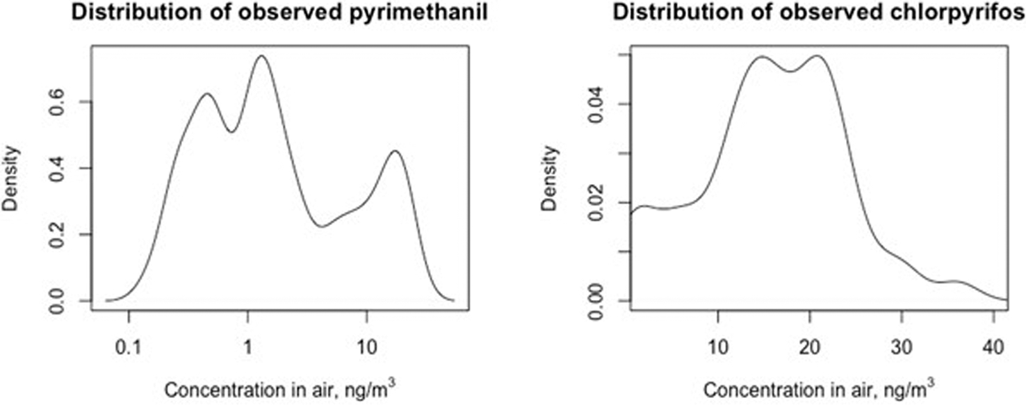
Distributions of measured pyrimethanil and chlorpyrifos concentrations in air (ng/m3), n = 48 from 12 schools in Matina County, Costa Rica.

The estimated parameters from the two spatiotemporal models for pesticide air concentrations are shown in Table 2. Both the pyrimethanil and chlorpyrifos concentrations exhibit μ terms that capture substantial variability compared to the E_t terms and are much more correlated across space, with spatial range parameters of 0.40 and 0.32°, for pyrimethanil and chlorpyrifos, respectively. Intuitively, the autoregressive parameter ϕ is significant and positive in both models, indicating correlation over time.

Table 2. Spatiotemporal parameter estimates and 95% credible intervals.

Both pyrimethanil and chlorpyrifos are measured in ng/m³.

Parameter*	Log10 pyrimethanil	Chlorpyrifos
β0	0.01 (−4.49, 4.36)	3.38 (−15.1, 19.0)
${\mathrm{\sigma }}_{\mathrm{\mu }}^2$	6.07 (0.44, 28.6)	608 (64.3, 2,721)
ρμ	0.40 (0.03, 1.81)	0.32 (0.04, 1.38)
φ	0.36 (0.10, 0.66)	0.51 (0.17, 0.96)
${\mathrm{\sigma }}_{\mathrm{E}}^2$	0.05 (0.03, 0.07)	7.58 (1.09, 12.9)
ρE	0.01 (0.01, 0.02)	0.02 (0.01, 0.03)

^*β₀ is the global mean for the time-invariant GP μ; _μ and ${\mathrm{\sigma }}_{\mathrm{\mu }}^2$ are the spatial range and variance of the time-invariant GP μ. ρ_E and ${\mathrm{\sigma }}_{\mathrm{E}}^2$ are the spatial range and variance of the time-specific GPs E_t.

The imputed values at the air measurement locations given by these estimated parameters are shown in Fig. 4. This figure shows the original observed values at the 12 different air measurement locations, and the values after the missing data had been imputed. Fig. S5 of the Supplement gives the distributions of both the observed and imputed exposures. These imputed values largely revert to the mean of the observed values at each location. Note that for pyrimethanil, the Kriging equations specify the expected mean of log₁₀ pyrimethanil, which is then exponentiated with base 10 to obtain imputed values. These values can be interpreted as the estimated median (non-logged) pyrimethanil values given by the Kriging distribution; however, they differ from the mean pyrimethanil value, due to its highly skewed distribution. With respect to the accuracy results for the validation of the spatiotemporal models: for pyrimethanil, the (non-logged) average absolute error was 3.4, which is close to half the observed standard deviation of 6.5 in the air measurements. For chlorpyrifos, the average absolute error was 7.4, slightly below the observed standard deviation of 8.1. Given the small original sample size from which the test set was taken (70% of 48 data points), these numbers give confidence that the full models have reasonable predictive accuracy. Fig. S6 in the Supplementary Material illustrates this accuracy. The spatiotemporal model shows the trend reasonably well, although does deviate for several datapoints. Moreover, the predictions tend to revert towards the mean, giving over-predictions for small values, and under-predictions for large values. This is particularly apparent in the large chlorpyrifos test set values, which are well above any of the training set values.

Fig. 4. Observed and imputed pyrimethanil and chlorpyrifos concentrations measured in air (ng/m³).

The left two figures show the observed values of pyrimethanil and chlorpyrifos across time at each location. As seen by breaks in the lines, there is substantial missing data. The right two figures impute the missing values for these data using the spatiotemporal model described in the Statistical Analysis Section.

Fig. 5 illustrates the mean levels and uncertainty associated with the two μ fields, which represent the time-averaged exposures across space. The two left figures give the average level of μ(s) for log₁₀ pyrimethanil and chlorpyrifos. Log₁₀pyrimethanil in air was relatively high at two locations, whilst chlorpyrifos in air also was high at two locations, but more uniformly distributed throughout the study area, and its concentrations followed a normal distribution. The two right figures give the standard deviation of μ(s) for log₁₀ pyrimethanil and chlorpyrifos, reflecting the uncertainty in the mean. Uncertainty is lowest at locations with observed air measurements and highest at the extreme borders of the area.

The final models selected by backwards selection are given in Tables 3 and 4. With respect to pyrimethanil, as both air pyrimethanil and OHP were log₁₀transformed prior to statistical analysis because of their distributions, a 10% increase in pyrimethanil air concentrations was associated with a 5.7% (95% CI 4.6, 6.8) increase in urinary OHP. The two additional covariates selected by backwards selection were “log₁₀ distance to the banana plantation” and “eats rice and beans 15 or more times a week”. Residential distance from the banana plantation was inversely associated with OHP, with each 10% increase in distance (meters), OHP decreased −0.7% (95% CI −1.2, −0.3). Eating rice and beans 15 or more times a week was associated with a 23% decrease in OHP. Lastly, the fixed effects explain 15% of the response variability of which pyrimethanil air concentrations explained 13%. The explained variability increased to 28% once random effects were included. For chlorpyrifos, an increase in 1 ng/m³ of chlorpyrifos in air was associated with a 1.5% (95% CI 0.2, 2.8) increase in urinary TCPy, all else being equal. As mentioned previously, chlorpyrifos air concentrations were not log₁₀-transformed as these followed a normal distribution. In addition, the binary variable “works for a banana plantation or other agricultural job (current)” was selected by the backwards modelling and associated with a 21% (95% CI −1.9, 48.9) increase in TCPy. These fixed effects explained only 1.2% of the variance, and after including the person-level random effects 37% of response variability.

Table 3.

Log₁₀ OHP model chosen by variable selection, with random effects (n = 894)^§.

Fixed effects		Random Effects		Explained variability a
Variables	% change in OHP (95% CI)	Person	Residuals	$R_m^2$	$R_c^2$
Intercept	−0.46*** (−0.58, −0.33)	0.06	0.31	0.15	0.28
For each 10% increase in pyrimethanil concentration (ng/m3)	5.72*** (4.64, 6.82)b
For each 10% increase in distance to banana plantation (meters)	−0.72** (−1.17, −0.27)b
For eating rice and beans 15 times a week or more	−23.0* (−38.2, −4.03)c

^a${\mathrm{R}}_{\mathrm{m}}^2$ represents variability explained by the fixed effects; ${\mathrm{R}}_{\mathrm{c}}^2$ represents variability explained by both fixed and random effects.

^bThe β estimates for pyrimethanil and distance to plantation reflect % increase in OHP per 10% increase in pyrimethanil concentration and distance to plantation, respectively.

^cThe β estimate for eating rice and beans reflects % increase in OHP expected for women who eat rice and beans 15 + times a week compared to those that do not.

^***denotes significance at the 0.001 level

^**the 0.01 level

^*the 0.05 level.

^§The unadjusted estimates (95% CI) from the regression for the intercept = −0.65 (−0.71, −0.59), and for each 10% increase in pyrimethanil concentration = 5.83 (4.84, 6.84).

Table 4.

Log10 TCPy model chosen by variable selection, with random effects (n = 915)^§.

Fixed effects		Random Effects		Explained variability a
Variables	% change in TCPy (95% CI)	Person	Residuals	$R_m^2$	$R_c^2$
Intercept	0.15*** (0.06, 0.23)	0.04	0.07	0.01	0.37
For each 1-unit increase in chlorpyrifos concentration in air (ng/m3)	1.45* (0.16, 2.75)b
For women working in agriculture	20.8 (−1.94, 48.9)c

^***denotes significance at the 0.001 level

^**the 0.01 level

^*the 0.05 level.

^a${\mathrm{R}}_{\mathrm{m}}^2$ represents variability explained by the fixed effects; ${\mathrm{R}}_{\mathrm{c}}^2$ represents variability explained by both fixed and random effects.

^bThe β estimate for chlorpyrifos reflects % increase in TCPy per ng/m³ increase in the chlorpyrifos air concentration.

^cThe β estimate for women working in agriculture reflects % increase in TCPy expected for women in agriculture compared to those not in agriculture.

^§The unadjusted estimates (95% CI) from the regression for the intercept=0.16 (0.09, 0.23), and for each ng increase in chlorpyrifos concentration=1.46 (0.38, 2.55).

4. Discussion

Pesticide air concentrations explained some of the variability of urinary pesticide metabolite concentrations, particularly for the fungicide pyrimethanil which is applied by light aircrafts, and only slightly for chlorpyrifos applied by pretreated bags used to cover the bananas bunches when ripening. Air pyrimethanil was highest very near banana plantations and its concentrations followed a lognormal distribution, while the insecticide chlorpyrifos was also higher near banana plantations but distributed more uniformly throughout the study area and its concentrations followed a normal distribution. This coincided with our finding that women who lived at a longer distance from banana plantations had lower urinary fungicide concentrations (OHP) than women living near banana plantations. For TCPy, residential distance was not selected by the backward modeling. When including it manually, it also showed an inverse association, though this association was imprecise: for each 10% increase in residential distance TCPy decreases −0.11% (95% CI −0.43, 0.21) (data not shown). The more uniform distribution of chlorpyrifos exposure is reflected by its higher detection frequency and higher median concentrations in both air (>LOD = 98%, median = 15.62 ng/m³) and of its metabolite in urine (>LOD 100%, median = 1.63 μg/L) while for pyrimethanil, detection frequency was lower (>LOD 81%, median = 1.33 ng/m³ in air; >LOD 87%, median = 0.39 μg/L in urine). The chlorpyrifos-treated bags are likely to produce a relatively constant emission to air, as chlorpyrifos is moderately volatile, while aerial application of the non-volatile fungicide pyrimethanil is expected to particularly expose women living near the plantations, possibly by inhaling aerosols near aerial application sites (Córdoba Gamboa et al., 2020). Furthermore, women working at banana plantations or performing other agricultural work had slightly higher chlorpyrifos exposures, which can be explained as they will spend more time near chlorpyrifos-treated bags as compared to women who do not perform these jobs. We did not observe this tendency for the fungicide pyrimethanil, while we did in a previous analysis for the also aerially applied fungicide mancozeb (van Wendel de Joode et al., 2014). Possibly, because mancozeb is used more extensively (26.14 kg active ingredient (a.i.)/hectare (ha) per year) than pyrimethanil (0.60 kg a.i./ha per year) (Bravo et al., 2013), which is also reflected by the overall higher median urinary concentrations of urinary ethylene thiourea (median = 3.0 μg/L) (van Wendel de Joode et al., 2014), the main metabolite of mancozeb, as compared to urinary OHP (median = 0.4 μg/L). Finally, eating rice and beans more frequently was associated with lower OHP, a finding we cannot explain.

One important consideration in interpreting these results is the low ICC values shown for log₁₀ OHP and log₁₀ TCPy (0.28 and 0.37). This ICC for TCPy is generally in line with other estimates in the literature (Fortenberry et al., 2014; Li et al., 2019; van Wendel de Joode et al., 2016), although is significantly below the estimate from Klimowska et al. (2020). The ICC can be interpreted as the correlation between measurements from the same person, or equivalently, the proportion of total variability coming from inter-person variation. In this case, these low correlations imply that urine measurements may change across visits for the same person. This is a key limitation when estimating the contribution of air exposure to urinary levels, as it means the response in the final regressions will contain significant noise, and the relative air contribution to urine concentrations will possibly be attenuated. This is likely one reason for the low R² values in the regressions. One solution to address this in future studies would be to collect more samples for each person. (The air measurements for log₁₀ pyrimethanil and chlorpyrifos showed much higher ICCs: 0.88 and 0.80, respectively, and are thus less of a concern).

Few researchers have studied the relation between pesticides air concentration and urinary pesticide metabolites in agricultural populations. Raherison and colleagues (Raherison et al., 2019) measured pesticides in air and urinary metabolites in vineyards in France, nevertheless, they did not analyze if pesticide air concentration explained the variability of urinary pesticide metabolites. Another study conducted in Belgium, measured current-use pesticides in air, their metabolites, and sometimes parent compounds, in children’s urine (Pirard et al., 2020). The authors concluded air did not seem to contribute substantially to internal exposures as urinary metabolites of pesticides frequently detected in air were not frequently detected in urine and vice-versa. Yet, the comparisons between external and internal exposure measurements were limited by the relatively low detection frequency of specific pesticides in either air or urine.

The strength of this analysis lies in the unique variables measured over time and space, which allows for a novel look at the relationship between air concentrations of pyrimethanil and chlorpyrifos with urinary pesticide metabolite concentrations of OHP and TCPy. In the same vein, however, a key limitation of this analysis is the relatively small size of the dataset with which to examine these relationships. More comprehensive data across space and time would undoubtedly increase the accuracy of the spatiotemporal model, and better isolate the association between these variables. Furthermore, our analysis was limited to static environmental air measurements, instead of personal air measurements, and did not include assessment of dermal exposure which may be relevant not only for occupational pesticide exposure but also environmental pesticide exposure (van Wendel de Joode et al., 2012). Nevertheless, we were able to address variables related to food intake, which is important as diet is a common source of pesticide exposure (McKone et al., 2007). Yet, in this study consumption of fruits and vegetables did not seem to increase exposure to chlorpyrifos or pyrimethanil.

5. Conclusions

Despite differences in exposure assessment approach (environmental versus personal, not always covering same period) and intra-class correlation coefficients (high for air samples, at least these two pesticides, versus low for urinary metabolites), air measurements still explained some of the variability of urinary pesticide metabolite concentrations which suggest pregnant women participating in the ISA study are environmentally exposed to pesticides used at banana plantations by inhalation. We recommend plantation owners implement measures to reduce these exposures, such as increasing distance between banana plantations and residential areas, including schools, and replacing the use of synthetic pesticides with less toxic alternatives.

In conclusion, the Bayesian spatiotemporal models were useful to extrapolate pyrimethanil and chlorpyrifos air concentrations across space and time. Our results suggest inhalation of pyrimethanil and chlorpyrifos is a pathway of environmental exposure. PAS seems a useful technique to monitor environmental current-use pesticide exposures. For future studies, we recommend increasing the number of locations of environmental air measurements, obtaining both air and urine measurement during the same period, and, ideally, including dermal exposure estimates as well.

References

- Bartón K, 2020. MuMIN: multi-model inference. R package version 1.43.17. [Google Scholar]
- Bernabò I, Guardia A, MacIrella R, Tripepi S, Brunelli E, 2017. Chronic exposures to fungicide pyrimethanil: Multi-organ effects on Italian tree frog (Hyla intermedia). Sci. Rep 7, 1–16. 10.1038/s41598-017-07367-6. [DOI] [PMC free article] [PubMed] [Google Scholar]
- Bravo V, Malavassi E de la C, Herrera G, Ramírez F, 2013. Uso de plaguicidas en cultivos agricolas como agriculture pesticides use as tool for monitoring health. Uniciencia 27, 351–376. [Google Scholar]
- Britton W, Drew D, Holman E, Lowe K, Lowit A, Rickard K, Health Effect Division, 7509P, Office of Pesticide Programs, Tan, C., (NERL), N.E.R.L., Development, O. of R. an, 2016. Chlorpyrifos: Revised Human Health Risk Assessment for Registration Review, EPA-HQ-OPP-2015–0653-0454
- Córdoba Gamboa L, Solano Díaz K, Ruepert C, van Wendel de Joode B, 2020. Passive monitoring techniques to evaluate environmental pesticide exposure: Results from the Infant’s Environmental Health study (ISA). Environ. Res 184, 109243. doi: 10.1016/j.envres.2020.109243. [DOI] [PMC free article] [PubMed] [Google Scholar]
- Curl CL, Fenske RA, Kissel JC, Shirai JH, Moate TF, Griffith W, Coronado G, Thompson B, 2002. Evaluation of take-home organophosphorus pesticide exposure among agricultural workers and their children. Environ. Health Perspect 110, 787–792. 10.1289/ehp.021100787. [DOI] [PMC free article] [PubMed] [Google Scholar]
- Deziel NC, Freeman LEB, Graubard BI, Jones RR, Hoppin JA, Thomas K, Hines CJ, Blair A, Sandler DP, Chen H, Lubin JH, Andreotti G, Alavanja MCR, Friesen MC, 2017. Relative contributions of agricultural drift, para-occupational, and residential use exposure pathways to house dust pesticide concentrations: Meta-regression of published data. Environ. Health Perspect 125 (3), 296–305. 10.1289/EHP426. [DOI] [PMC free article] [PubMed] [Google Scholar]
- Deziel NC, Friesen MC, Hoppin JA, Hines CJ, Thomas K, Freeman LEB, 2015. A Review of Nonoccupational Pathways for Pesticide Exposure in Women Living in Agricultural Areas. Environ. Health Perspect 123 (6), 515–524. 10.1289/ehp.1408273. [DOI] [PMC free article] [PubMed] [Google Scholar]
- European Commission, 2020. COMMISSION REGULATION (EU) 2020/1085. Off. J. Eur. Union [Google Scholar]
- Fenske RA, Bradman A, Whyatt RM, Wolff MS, Barr DB, 2005. Lessons Learned for the Assessment of Children’s Pesticide Exposure: Critical Sampling and Analytical Issues for Future Studies. Environ. Health Perspect 113 (10), 1455–1462. 10.1289/ehp.7674. [DOI] [PMC free article] [PubMed] [Google Scholar]
- Food E, Authority S, 2019. Statement on the available outcomes of the human health assessment in the context of the pesticides peer review of the active substance chlorpyrifos. EFSA J 17. doi: 10.2903/j.efsa.2019.5809. [DOI] [PMC free article] [PubMed] [Google Scholar]
- Fortenberry GZ, Meeker JD, Sánchez BN, Barr DB, Panuwet P, Bellinger D, Schnaas L, Solano-González M, Ettinger AS, Hernandez-Avila M, Hu H, Tellez-Rojo MM, 2014. Urinary 3, 5, 6-trichloro-2-pyridinol (TCPY) in pregnant women from Mexico City: distribution, temporal variability, and relationship with child attention and hyperactivity. Int. J. Hyg. Environ. Health 217 (2–3), 405–412. [DOI] [PMC free article] [PubMed] [Google Scholar]
- Hamsan H, Ho YB, Zaidon SZ, Hashim Z, Saari N, Karami A, 2017. Occurrence of commonly used pesticides in personal air samples and their associated health risk among paddy farmers. Sci. Total Environ 603–604, 381–389. 10.1016/j.scitotenv.2017.06.096. [DOI] [PubMed] [Google Scholar]
- Han D-H, 2011. Airborne concentrations of organophosphorus pesticides in Korean pesticide manufacturing/ formulation workplaces. Ind. Health 49 (6), 703–713. 10.2486/indhealth.MS1304. [DOI] [PubMed] [Google Scholar]
- Hines CJ, Deddens JA, Coble J, Kamel F, Alavanja MCR, 2011. Determinants of captan air and dermal exposures among orchard pesticide applicators in the agricultural health study. Ann. Occup. Hyg 55, 620–633. 10.1093/annhyg/mer008. [DOI] [PMC free article] [PubMed] [Google Scholar]
- Hore P, Zartarian V, Xue J, Özkaynak H, Wang S-W, Yang Y-C, Chu P-L, Sheldon L, Robson M, Needham L, Barr D, Freeman N, Georgopoulos P, Lioy PJ, 2006. Children’s residential exposure to chlorpyrifos: Application of CPPAES field measurements of chlorpyrifos and TCPy within MENTOR/SHEDS-Pesticides model. Sci. Total Environ 366 (2–3), 525–537. 10.1016/j.scitotenv.2005.10.012. [DOI] [PubMed] [Google Scholar]
- Hurley PM, Hill RN, Whiting RJ, 1998. Mode of carcinogenic action of pesticides inducing thyroid follicular cell tumors in rodents. Environ. Health Perspect 106, 437–445. 10.1289/ehp.98106437. [DOI] [PMC free article] [PubMed] [Google Scholar]
- Kawahara J, Horikoshi R, Yamaguchi T, Kumagai K, Yanagisawa Y, 2005. Air pollution and young children’s inhalation exposure to organophosphorus pesticide in an agricultural community in Japan. Environ. Int 31 (8), 1123–1132. 10.1016/j.envint.2005.04.001. [DOI] [PubMed] [Google Scholar]
- Kim H-H, Lim Y-W, Yang J-Y, Shin D-C, Ham H-S, Choi B-S, Lee J-Y, 2013. Health risk assessment of exposure to chlorpyrifos and dichlorvos in children at childcare facilities. Sci. Total Environ 444, 441–450. 10.1016/j.scitotenv.2012.11.102. [DOI] [PubMed] [Google Scholar]
- Klimowska A, Amenda K, Rodzaj W, Wileńska M, Jurewicz J, Wielgomas B, 2020. Evaluation of 1-year urinary excretion of eight metabolites of synthetic pyrethroids, chlorpyrifos, and neonicotinoids. Environ. Int 145, 106119. 10.1016/j.envint.2020.106119. [DOI] [PubMed] [Google Scholar]
- Li AJ, Martinez-Moral M-P, Kannan K, 2019. Temporal variability in urinary pesticide concentrations in repeated-spot and first-morning-void samples and its association with oxidative stress in healthy individuals. Environ. Int 130, 104904. 10.1016/j.envint.2019.104904. [DOI] [PMC free article] [PubMed] [Google Scholar]
- Lozier MJ, Montoya JFL, del Rosario A, Martínez EP, Fuortes L, Cook TM, Sanderson WT, 2013. Personal air sampling and risks of inhalation exposure during atrazine application in honduras. Int. Arch. Occup. Environ. Health 86 (4), 479–488. 10.1007/s00420-012-0776-2. [DOI] [PubMed] [Google Scholar]
- McKone TE, Castorina R, Harnly ME, Kuwabara Y.u., Eskenazi B, Bradman A, 2007. Merging models and biomonitoring data to characterize sources and pathways of human exposure to organophosphorus pesticides in the Salinas Valley of California. Environ. Sci. Technol 41 (9), 3233–3240. 10.1021/es061844710.1021/es0618447.s001. [DOI] [PubMed] [Google Scholar]
- Mora AM, Córdoba L, Cano JC, Hernandez-Bonilla D, Pardo L, Schnaas L, Smith DR, Menezes-Filho JA, Mergler D, Lindh CH, Eskenazi B, de Joode B van W, 2018. Prenatal mancozeb exposure, excess manganese, and neurodevelopment at 1 year of age in the infants’ environmental health (ISA) study. Environ. Health Perspect 126. doi: 10.1289/EHP1955. [DOI] [PMC free article] [PubMed] [Google Scholar]
- Mora AM, Hoppin JA, Córdoba L, Cano JC, Soto-Martínez M, Eskenazi B, Lindh CH, van Wendel de Joode B, 2020. Prenatal pesticide exposure and respiratory health outcomes in the first year of life: Results from the infants’ Environmental Health (ISA) study. Int. J. Hyg. Environ. Health 225, 113474. doi: 10.1016/j.ijheh.2020.113474. [DOI] [PMC free article] [PubMed] [Google Scholar]
- Nakagawa S, Schielzeth H, O’Hara RB, 2013. A general and simple method for obtaining R 2 from generalized linear mixed-effects models. Methods Ecol. Evol 4 (2), 133–142. 10.1111/j.2041-210x.2012.00261.x. [DOI] [Google Scholar]
- Norén E, Lindh C, Rylander L, Glynn A, Axelsson J, Littorin M, Faniband M, Larsson E, Nielsen C, 2020. Concentrations and temporal trends in pesticide biomarkers in urine of Swedish adolescents, 2000–2017. J. Expo. Sci. Environ. Epidemiol 30 (4), 756–767. 10.1038/s41370-020-0212-8. [DOI] [PMC free article] [PubMed] [Google Scholar]
- Pirard C, Remy S, Giusti A, Champon L, Charlier C, 2020. Assessment of children’s exposure to currently used pesticides in wallonia. Belgium. Toxicol. Lett 329, 1–11. 10.1016/j.toxlet.2020.04.020. [DOI] [PubMed] [Google Scholar]
- Plummer M, 2003. JAGS: A Program for Analysis of Bayesian Graphical Models Using Gibbs Sampling In: Proceedings of the 3rd International Workshop on Distributed Statistical Computing. Vienna, Austria, pp. 1–10. [Google Scholar]
- R Core Team, 2020. R: A language and environment for statisticalcomputing
- Raherison C, Baldi I, Pouquet M, Berteaud E, Moesch C, Bouvier G, Canal-Raffin M, 2019. Pesticides Exposure by Air in Vineyard Rural Area and Respiratory Health in Children: A pilot study. Environ. Res 169, 189–195. 10.1016/j.envres.2018.11.002. [DOI] [PubMed] [Google Scholar]
- Rodríguez T, Younglove L, Lu C, Funez A, Weppner S, Barr DB, Fenske RA, 2006. Biological monitoring of pesticide exposures among applicators and their children in Nicaragua. Int. J. Occup. Environ. Health 12 (4), 312–320. 10.1179/oeh.2006.12.4.312. [DOI] [PubMed] [Google Scholar]
- Roitzsch M, Schäferhenrich A, Baumgärtel A, Ludwig-Fischer K, Hebisch R, Göen T, 2019. Dermal and Inhalation Exposure of Workers during Control of Oak Processionary Moth (OPM) by Spray Applications. Ann. Work Expo. Heal 63, 294–304. 10.1093/annweh/wxy108. [DOI] [PubMed] [Google Scholar]
- Smith MN, Workman T, McDonald KM, Vredevoogd MA, Vigoren EM, Griffith WC, Thompson B, Coronado GD, Barr D, Faustman EM, 2017. Seasonal and occupational trends of five organophosphate pesticides in house dust. J. Expo. Sci. Environ. Epidemiol 27 (4), 372–378. 10.1038/jes.2016.45. [DOI] [PubMed] [Google Scholar]
- Taneepanichskul N, Norkaew S, Siriwong W, Siripattanakul-Ratpukdi S, Maldonado Pérez HL, Robson MG, 2014. Organophosphate pesticide exposure and dialkyl phosphate urinary metabolites among chili farmers in northeastern Thailand. Rocz. Panstw. Zakl. Hig 65, 291–299. [PubMed] [Google Scholar]
- Tsakirakis AN, Kasiotis KM, Charistou AN, Arapaki N, Tsatsakis A, Tsakalof A, Machera K, 2014. Dermal & inhalation exposure of operators during fungicide application in vineyards. Evaluation of coverall performance. Sci. Total Environ 470–471, 282–289. 10.1016/j.scitotenv.2013.09.021. [DOI] [PubMed] [Google Scholar]
- van Wendel de Joode B, Barraza D, Ruepert C, Mora AM, Córdoba L, Öberg M, Wesseling C, Mergler D, Lindh CH, 2012. Indigenous children living nearby plantations with chlorpyrifos-treated bags have elevated 3,5,6-trichloro-2-pyridinol (TCPy) urinary concentrations. Environ. Res 117, 17–26. 10.1016/j.envres.2012.04.006. [DOI] [PubMed] [Google Scholar]
- van Wendel de Joode B, Mora A, Córdoba L, Cano J, Quesada R, Faniband M, Wesseling C, Ruepert C, Öberg M, Eskenazi B, Mergler D, Lindh C, 2014. Aerial Application of Mancozeb and Urinary Ethylene Thiourea (ETU) Concentrations among Pregnant Women in Costa Rica: The Infants’ Environmental Health Study (ISA). Environ. Health Perspect 122, 1321–1328. doi: 10.1289/ehp.122-a321. [DOI] [PMC free article] [PubMed] [Google Scholar]
- van Wendel de Joode B, Mora AM, Lindh CH, Hernández-Bonilla D, Córdoba L, Wesseling C, Hoppin JA, Mergler D, 2016. Pesticide exposure and neurodevelopment in children aged 6–9 years from Talamanca, Costa Rica. Cortex, 85, pp.137–150. [DOI] [PubMed] [Google Scholar]
- Wang Y, Wu S, Chen J, Zhang C, Xu Z, Li G, Cai L, Shen W, Wang Q, 2018. Single and joint toxicity assessment of four currently used pesticides to zebrafish (Danio rerio) using traditional and molecular endpoints. Chemosphere 192, 14–23. 10.1016/j.chemosphere.2017.10.129. [DOI] [PubMed] [Google Scholar]
- Weppner S, Elgethun K, Lu C, Hebert V, Yost MG, Fenske RA, 2006. The Washington aerial spray drift study: Children’s exposure to methamidophos in an agricultural community following fixed-wing aircraft applications. J. Expo. Sci. Environ. Epidemiol 16 (5), 387–396. 10.1038/sj.jea.7500461. [DOI] [PubMed] [Google Scholar]
- Wolak ME, Fairbairn DJ, Paulsen YR, 2012. Guidelines for estimating repeatability. Methods Ecol. Evol 3, 129–137. 10.1111/j.2041-210X.2011.00125.x. [DOI] [Google Scholar]
- Yusa V, Millet M, Coscolla C, Roca M, 2015. Analytical methods for human biomonitoring of pesticides. A review. Anal. Chim. Acta 891, 15–31. 10.1016/j.aca.2015.05.032. [DOI] [PubMed] [Google Scholar]
Associated Data
This section collects any data citations, data availability statements, or supplementary materials included in this article.