

Abstract
To suppress the streak artifacts in images reconstructed from sparse-view projections in computed tomography (CT), a residual, attention-based, dense UNet (RAD-UNet) deep network is proposed to achieve accurate sparse reconstruction. The filtered back projection (FBP) algorithm is used to reconstruct the CT image with streak artifacts from sparse-view projections. Then, the image is processed by the RAD-UNet to suppress streak artifacts and obtain high-quality CT image. Those images with streak artifacts are used as the input of the RAD-UNet, and the output-label images are the corresponding high-quality images. Through training via the large-scale training data, the RAD-UNet can obtain the capability of suppressing streak artifacts. This network combines residual connection, attention mechanism, dense connection and perceptual loss. This network can improve the nonlinear fitting capability and the performance of suppressing streak artifacts. The experimental results show that the RAD-UNet can improve the reconstruction accuracy compared with three existing representative deep networks. It may not only suppress streak artifacts but also better preserve image details. The proposed networks may be readily applied to other image processing tasks including image denoising, image deblurring, and image super-resolution.
Keywords: Attention mechanism, Residual connection, Sparse-view CT, Streak artifacts, UNet
Introduction
Computed tomography (CT) is the most widely used medical imaging technology. However, the X-ray radiation to the human body during CT scan increases the risk of disease to the patients. Therefore, low-dose CT has become the mainstream direction of the current CT study. There are two implementation methods for low-dose CT. One is to reduce the radiation dose at each projection-view, and the other is to collect projections only from sparse views. Reconstructing image from sparse-view projections is the so-called sparse reconstruction. This paper focuses on the second low-dose CT reconstruction method, i.e., sparse reconstruction. Analytical methods, such as filtered back projection (FBP) [1] algorithm, are the mainstream algorithms for commercial CT imagers. But, sparse reconstruction via these algorithms may produce serious streak artifacts, which can affect subsequent medical diagnosis. So, people explored many accurate CT sparse-reconstruction algorithms in the last twenty years.
In 2006, Sidky et al. proposed a total variation (TV) minimization algorithm that is an iterative algorithm based on compressed sensing (CS) [2] and capable of achieving accurate CT sparse reconstruction [3, 4]. Since then, many modified TV algorithms have been proposed to further improve the accuracy of sparse reconstruction, such as adaptive weighted TV (awTV) [5], edge-preserving TV (EPTV) [6], anisotropic TV (aTV) [7], high order TV (HOTV) [8], non-local TV (NLTV) [9], and total p-variation (TpV) [10]. These TV algorithms have strongly promoted the development of sparse reconstruction. In addition, other reconstruction algorithms based on CS have also been deeply studied, such as the methods based on dictionary learning [11] and the methods based on rank minimization [12].
The deep learning (DL)-based image reconstruction method brings a new perspective to CT sparse reconstruction, which can be roughly divided into four types [13, 14].
The first type is end-to-end direct reconstruction, which directly allows the deep network to learn the mapping between the projections and the reconstructed images, and AUTOMAP, which was a typical representative of this method [15]. However, this method is not suitable for high-resolution image reconstruction and high-dimensional image reconstruction. For example, in 3D cone-beam CT reconstruction, both the projections and the 3D object are very large. By using this method to reconstruct image, the network will be very huge, and massive training data are required. These factors limit the application of this method.
The second one is the projection domain processing method, which essentially uses DL-based method to process the projection sinogram. Lee et al. used convolutional neural networks (CNN) to interpolate the sparse sampled sinogram of CT images to obtain complete projections [16]. Dong et al. also applied the residual UNet to perform this task, which not only improved the image quality but also greatly reduced the computational cost [17].
The third one is the combination of the DL-based method and the iterative method, which essentially changes the iterative process into a network form, and then learns the regularization term and some reconstruction parameters. Chen et al. proposed the LEARN network, which used CNN to learn the regularization term and some parameters in the iterative process at the same time. The accuracy of the reconstructed image was higher than the traditional TV method [18]. The ADMM-Net proposed by Yang et al. combined the ADMM algorithm with CNN for image reconstruction, which had an effective improvement in the accuracy and speed of image reconstruction [19].
The fourth one is the image domain processing method, which essentially uses the deep networks to process the low-quality images reconstructed by the analytical methods. The RED-CNN proposed by Chen et al. combined deconvolution [20] and residual learning [21], achieving excellent results in low-dose CT reconstruction [22]. Wolterink et al. used the generative adversarial networks (GANs) [23] to achieve improvement in low-dose CT reconstruction [24]. Han et al. proved that learning streak artifacts was easier than learning the original signal directly and proposed a deep residual learning method based on UNet [25]. The proposed method estimated streak artifacts for obtaining high-quality CT images [26]. The FBPConvNet proposed by Jin et al. combined the residual UNet with the FBP algorithm to suppress the streak artifacts in CT sparse reconstruction. Compared with the traditional TV algorithm, this method suppressed the streak artifacts more effectively [27]. The DD-Net proposed by Zhang et al. combined dense connection [28] with deconvolution, overcame the problems of gradient disappearance, gradient explosion, and increased the size of model parameters to improve the training performance of network [29]. Han and Ye evaluated the limitations of image edge-blur caused by UNet and proposed a multi-resolution deep learning network: dual frame and the tight frame UNets, which enhanced the high-frequency features of the image. The quality of the image reconstruction is better than the traditional TV algorithm [30]. The FD-UNet proposed by Steven et al. introduced dense connection in the contraction and expansion paths of the UNet to suppress streak artifacts, enhancing the flow of information and feature reusing [31].
A study on the DL-based method shows that residual learning can guarantee good performance while training deeper networks and to a certain extent solves the problems of gradient disappearance and gradient explosion of deep neural networks [21]. Dense connection increases the feature reusing of shallow networks in deep networks and improves the expressive capability [28]. Attention mechanism emphasizes useful information by weighting the space or channel information and improves the network performance [32–34]. Perceptual loss can make up for the shortcomings of the mean square error (MSE) describing pixel-level loss and improves the accuracy of DL-based image processing [35–37].
Motivated by these important insights, this paper intends to combine these advantages to design a residual, attention-based, dense UNet (RAD-UNet), which is used to suppress streak artifacts in CT images reconstructed by the FBP algorithm.
The “Methods” section introduces the proposed RAD-UNet. The “Results” section introduces the experiments and analysis, and finally, we give a concise conclusion in “Conclusion”.
Methods
This section first introduces the CNN-based CT sparse reconstruction method, then introduces the proposed RAD-UNet, and finally introduces three DL-based sparse reconstruction algorithms that are compared with the proposed method.
The CNN-based CT Sparse Reconstruction Method
CNN is suitable for image processing, which can well express the nonlinear mapping between input and output images. The CNN-based CT sparse reconstruction framework is shown in Fig. 1. First, we use the FBP algorithm to reconstruct the CT image, which has streak artifacts. Then, we use the CNN to suppress streak artifacts. The CT image with streak artifacts, , is the input of the network, and the corresponding high-quality CT image, , is the label of the network. The network can learn the mapping from to , expressed by . The trained network is the similar network expression of the function . Streak artifacts are complex nonlinear artifacts and are not uniformly distributed in the CT image. They are difficult to be modeled as mathematical model. The DL-based method learns the characteristics of streak artifacts from a large amount of training data, which has the potential to achieve accurate sparse reconstruction.
Fig. 1.
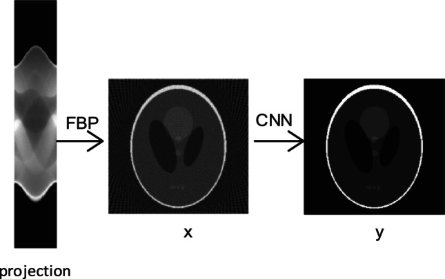
The workflow of CNN-based sparse CT reconstruction
RAD-UNet and Loss Function Design
A residual, attention-based, dense UNet (RAD-UNet) network for CT sparse reconstruction is shown in Fig. 2. The network input is the CT image of streak artifacts.
Fig. 2.

The structure of the RAD-UNet network
On the left of the network, the first convolution unit (here we call the operations between down-sampling layers as a convolution unit) consists of a 3 × 3 convolutional layer of 32-channels, a batch normalization (BN) layer, a rectified linear unit (ReLU) activation layer, and a residual, attention-based, dense (RAD) block operation. The other 4 convolution units only contain a RAD block operation.
On the right of the network, the output after each up-sampling layer is concatenated with the feature-map of the same size on the left of the network, and then, a 1 × 1 convolutional layer, a BN layer, a ReLU layer, and a residual dense (RD) block operation are followed. The 1 × 1 convolution operation reduces the number of channels into times of the original channels, and the RD block operation doubles the number of channels. The up-sampling operation is implemented by the transposed convolution, with the size of the convolution kernel being 4 × 4 and the stride being 2.
The last layer of the last convolution unit is a 1 × 1 convolution layer, and the channel number is 1, which is used to output images. In addition, a residual connection is added between the input and output of the network. In this way, the entire deep network is actually learning the mapping from the images of streak artifacts to the streak artifacts.
A RAD block with 32-channel input and 64-channel output is shown in Fig. 3. It is the RAD block in the first convolution unit and the RAD blocks in other units have a similar structure. From Fig. 3, we may see that the RAD block contains a total of 6 units. The first 4 units contain dense connections, and the specific change process of feature maps as shown in Fig. 3. The 5th unit is a channel attention module, as shown in Fig. 4. It learns a 64 × 1 channel attention weight and multiplies it with the input feature map of 64 channels. Then, it will obtain the feature-map that are enhanced at some specific channels. The 6th unit is a 1 × 1 convolutional layer. In addition, residual connection is added between the 4th unit and the 6th unit.
Fig. 3.

The structure of the RAD block
Fig. 4.

The attention module
The difference between the RD block and the RAD block is that the RD block does not have the 5th unit, i.e., the attention module.
The root mean square error (RMSE) loss function calculates the error between image pixels, which can be expressed as
| 1 |
Here, is the input image of size and y is the label-output image of size . is the number of training data. is the index of pixel in an image, and is the index of the training data.
The RMSE loss indicates the difference between pixels, so its capability of preserving image details is not very high. Therefore, the perceptual loss is added to calculate the difference between image features to improve the fitting capability of the proposed network.
The perceptual network uses the VGG-16 network trained on the ImageNet database. The perceptual loss can be expressed as
| 2 |
Here, represents the pre-trained VGG-16 network.
The loss function we used can be expressed as
| 3 |
Here, is a parameter to balance the strength between the two loss functions. We set it as 0.01 in this work to achieve the best performance.
Comparison Network
This paper uses three representative networks, RED-CNN, FBPConvNet, and FD-UNet as comparison network of the proposed RAD-UNet.
The RED-CNN combined residual connection and deconvolution, achieving accurate CT image denoising [22]. The FBPConvNet is actually the classical residual UNet, which achieved excellent results in sparse CT reconstruction [27]. The FD-UNet added dense connection in the contraction and expansion paths of the classic UNet to suppress the streak artifacts in images [31].
Results
The Construction of Dataset
In order to investigate the performance of the proposed RAD-UNet method, 2000 high-quality CT images including the head, thoracic cavity, and abdominal cavity are selected from the public CT image data set TCIA (https://www.cancerimagingarchive.net/). The image size is 512 × 512. The sparse-view projections are obtained by using radon transform on these CT images, and then, the FBP algorithm is used to reconstruct images from the sparse-view projections, which have streak artifacts. The reconstructed images are the input images, whereas the high-quality CT images are the label-images. Among them, 1900 CT image-pairs are selected as the training set, 50 CT image-pairs are used as the validation set, and 50 CT image-pairs are used as the test set. To fit for the size of GPU memory, we divide each CT image into 16 sub-images of size 128 × 128. Thus, the input and output images are both of size 128 × 128.
Hyper-parameters Setting
In these experiments, the RED-CNN, FBPConvNet, and FD-UNet methods use the RMSE loss function. The RAD-UNet uses the loss function combining RMSE and perceptual loss. The other parameters remain the same. All networks use Adam optimization algorithm ( = 0.5, = 0.999), the number of iterations is 15,000, and the initial learning rate is 0.0002. After 10,000 iterations, the learning rate decreases slowly and finally drops to 0.0001. The mini-batch size is 16. All convolution kernel weights initialization methods use the initialization method proposed by He et al. [38].
The CPU used is Inter(R) Xeon(R) CPU E5-2620 v4 @ 2.10 GHz, and the GPU is NVIDIA GeForce GTX 1080 Ti. These experiments are implemented by Python language based on the Keras framework. The RAD-UNet network training time is about 8 h; the other networks training time is about 7 and a half hours.
Results
This section shows the results of three experiments. First, the proposed RAD-UNet method is compared with the three existing methods. Then the comparison of the RAD-UNet reconstructions of different projection sparsity situations is performed. Finally, comparisons are performed between the proposed networks without any of the four mechanisms: (1) multi-loss mechanism, (2) dense connection mechanism, (3) residual learning mechanism, and (4) attention mechanism.
Comparison of Sparse Reconstruction Capability
To explore the performance of the RAD-UNet in sparse CT reconstruction, we compare it with the RED-CNN, FBPConvNet, and FD-UNet networks.
For each high-quality image in the whole dataset, 60 projections are uniformly collected in the range of [0, π] according to the parallel beam scan configuration. They are generated by use of the radon function in Matlab. Then, we use the FBP algorithm, i.e., the iradon function, to reconstruct image from the 60 projections. The reconstructed image and the truth image, i.e., the high-quality image, constitute the image-pair, one of which is the input of these network, and the other one of which is the output-label image of these network.
The reconstructed images are shown in Fig. 5. From Fig. 5, we may see that FBP-images have obvious streak artifacts, and RED-CNN-images still have some streak artifacts. The artifacts in FBPConvNet-images, FD-UNet-images, and RAD-UNet-images are significantly reduced. The RAD-UNet-images appear to preserve more image details. Figure 6 shows the enlarged images corresponding to the red box of Fig. 5. The red circle area in Fig. 6 is the main observation area. It can be seen from Fig. 6 that the texture structure of the RAD-UNet-images is more obvious and clearer.
Fig. 5.

The sparse reconstruction results of five reconstruction algorithms. The display window is [0, 1]
Fig. 6.

The enlarged images corresponding to the red-box in Fig. 5. The display window is [0, 1]
We choose mean standard deviation form of peak signal-to-noise ratio (PSNR), root mean square error (RMSE), and structural similarity (SSIM) as metrics to quantitatively evaluate the reconstruction quality of the test images. The quantitative comparison results are shown in Table 1. From it, we may see that the proposed network may achieve the most accurate reconstructions relative to these existing networks.
Table 1.
Comparison of PSNR, RMSE, and SSIM of the test images reconstructed by five reconstruction algorithms
| Reconstruction algorithm | FBP | RED-CNN | FBPConvNet | FD-UNet | RAD-UNet |
|---|---|---|---|---|---|
| RMSE | 0.0484 ± 0.0196 | 0.0358 ± 0.0172 | 0.0322 ± 0.0135 | 0.0291 ± 0.0155 | 0.0253 ± 0.0129 |
| SSIM | 0.5463 ± 0.1039 | 0.9443 ± 0.0562 | 0.9624 ± 0.0333 | 0.9608 ± 0.0343 | 0.9669 ± 0.0287 |
| PSNR | 26.95 ± 3.3949 | 30.15 ± 5.8301 | 30.85 ± 5.3536 | 32.15 ± 5.8636 | 33.19 ± 5.4282 |
This experiment shows that the proposed network may achieve the best CT sparse reconstruction based on qualitative observation and quantitative evaluations.
Comparison of Reconstruction Performance of RAD-UNet of Different Sparse Levels
To explore the performance of RAD-UNet sparse reconstruction of different sparse levels. We collect 15, 30, 60, and 90 projections, and perform FBP reconstructions to construct dataset. Thus, sparser projections lead to image with more serious streak artifacts, whereas denser projections lead to image with lighter streak artifacts. We will investigate how the reconstruction capability change with the change of projection number.
The experimental results are shown in Fig. 7, in which the streak artifacts in these FBP images become lighter and lighter with the increase of projection number. It can be seen that when projection number is 15, the reconstructed RAD-UNet-image losses a lot of details. When projection number is 30, the reconstructed image still has obvious streak artifacts and losses some details. But when projection number is 60, the details preserved is increased significantly and we cannot see any streak artifact. When projection number is 90, the image quality may be further improved. Figure 8 shows the enlarged images corresponding to the red box of Fig. 7. The red circle area in Fig. 8 is the main observation area. It can be seen from Fig. 8 that the texture structure of 90 projections of the RAD-UNet-images is more obvious and clearer.
Fig. 7.

Comparison of images reconstructed by the RAD-UNet of different sparse levels. The display window is [0, 1]
Fig. 8.

The enlarged images corresponding to the red-box in Fig. 7. The display window is [0, 1]
The quantitative comparison results are shown in Table 2, which may support the change law found by the above qualitative observations.
Table 2.
PSNR, SSIM, and RMSE of the reconstructed test images of the RAD-UNet of different sparse levels
| RAD-UNet-15 | RAD-UNet-30 | RAD-UNet-60 | RAD-UNet-90 | |
|---|---|---|---|---|
| RMSE | 0.0462 ± 0.0280 | 0.0315 ± 0.0174 | 0.0253 ± 0.0129 | 0.0235 ± 0.0132 |
| SSIM | 0.9067 ± 0.0682 | 0.9451 ± 0.0436 | 0.9669 ± 0.0287 | 0.9718 ± 0.0275 |
| PSNR | 28.35 ± 6.1282 | 31.38 ± 5.5260 | 33.19 ± 5.4282 | 34.18 ± 6.1446 |
Clearly, lighter streak artifacts the FBP image has, the higher accurate reconstruction capability the proposed network will achieve.
Internal Comparison of the RAD-UNet Performance
To further explore the impact of the four mechanisms used in the RAD-UNet on reconstruction, we carry out the RAD-UNet reconstructions without using any of the four mechanisms, dense connection, residual learning, attention mechanism, and multi-loss mechanism. The number of projections is 60.
The reconstructed images are shown in Fig. 9. It can be seen that without-dense-connection image has the most serious streak artifacts and losses some details, without-residual-learning image and without-attention image have a slightly better effect in suppressing artifacts, but there are still some artifacts. The without-perceptual-loss image is the closest to the RAD-UNet image, which has the highest reconstruction accuracy. Figure 10 shows the enlarged images corresponding to the red box of Fig. 9. The red circle area in Fig. 10 is the main observation area. It can be seen from Fig. 10 that the texture structure of the without-perceptual-loss image of the RAD-UNet is more obvious and clearer.
Fig. 9.

The images reconstructed by the RAD-UNet without any of the four mechanisms. The red box indicates the suggested observation region. The display window is [0, 1]
Fig. 10.

The enlarged images corresponding to the red-box in Fig. 9. The display window is [0, 1]
Figure 11 shows the iteration behavior of the loss functions of the five networks. It can be seen from Fig. 11 that all the networks does not overfit during the training process. Compared with the RAD-UNet, the loss value of without-dense-connection is relatively large. The loss curve of without-residual-learning and without-attention-module has relatively large fluctuations. There is no comparability between the loss curve of without-perceptual-loss and RAD-UNet, because the meaning of loss function is different. In short, the loss curve of RAD-UNet fluctuates comparatively little and finally stabilized to a very small value.
Fig. 11.

The iteration behavior of the loss functions of the five networks
The results of quantitative analysis are shown in Table 3. Observing the data row by row, we may see that the PSNR and SSIM are in ascending order, whereas the RMSE is in descending order. This means the image quality is higher and higher from left to right. Clearly, the importance order is dense connection, residual learning, attention mechanism, and then perceptual loss.
Table 3.
PSNR, SSIM, and RMSE of the test images reconstructed by the RAD-UNet without any of the four mechanisms
| Without dense connection | Without residual learning | Without attention module | Without perceptual loss | RAD-UNet | |
|---|---|---|---|---|---|
| RMSE | 0.0280 ± 0.0144 | 0.0262 ± 0.0137 | 0.0263 ± 0.0142 | 0.0260 ± 0.0131 | 0.0253 ± 0.0129 |
| SSIM | 0.9429 ± 0.0536 | 0.9622 ± 0.0312 | 0.9645 ± 0.0307 | 0.9611 ± 0.0291 | 0.9669 ± 0.0287 |
| PSNR | 32.25 ± 5.3130 | 32.91 ± 5.3424 | 32.99 ± 5.4706 | 32.94 ± 5.4161 | 33.19 ± 5.4282 |
Conclusions
In this paper, we propose a RAD-UNet network to suppress the streak artifacts in the FBP-reconstructed images, which combines dense connection, residual learning, attention, and multi-loss mechanisms based on the classical UNet. It increases the depth of the network by dense connection, improves the training performance by residual connection, and improves the network fitting capability by attention and multi-loss mechanisms. This is because residual learning may effectively avoid the problems of gradient disappearance and gradient explosion, dense connection may make the network deeper and reuse information in the previous layers, attention mechanism may emphasize more useful information, and multi-loss mechanism can better describe the mapping from input to output.
Compared with the existing RED-CNN, FBPConvNet, and FD-UNet networks, the proposed RAD-UNet may better suppress streak artifacts and preserve the image texture and details. Also, we find that the RAD-UNet may improve its capability of suppressing streak artifacts with the increase of projection number. We should note that deep learning has its limitation, observing that any deep network will fail if the projection number is too small, for example, 10 in this study. Another insight we gained is that the mechanism used in the proposed network has different importance. The order from high to low is dense connection, residual learning, attention mechanism, and multi-loss mechanism.
The RAD-UNet has great potential in improving the accuracy of CT sparse reconstruction. In the future, we will further introduce adversarial mechanism into the RAD-UNet, explore more attention mechanisms and introduce more loss functions to achieve higher reconstruction accuracy. Currently, we are applying this network to 3D electron paramagnetic resonance imaging (EPRI) for evaluating the performance of the proposed network in this imaging modality via real data.
Author Contribution
All authors contributed to the study conception and design. Material preparation, data collection and analysis were performed by Congcong Du and Zhiwei Qiao. The first draft of the manuscript was written by Congcong Du and all authors commented on previous versions of the manuscript. All authors read and approved the final manuscript.
Funding
This work was supported in part by the Natural Science Foundation of China under grant 62071281, by the Central Guidance on Local Science and Technology Development Fund Project under grant YDZJSX2021A003, and by the Research Project Supported by Shanxi Scholarship Council of China under grant 2020-008.
Declarations
Competing Interests
The authors declare no competing interests.
Footnotes
Publisher's Note
Springer Nature remains neutral with regard to jurisdictional claims in published maps and institutional affiliations.
Contributor Information
Zhiwei Qiao, Email: zqiao@sxu.edu.cn.
Congcong Du, Email: 15535734519@163.com.
References
- 1.Pan X, Sidky EY, Vannier M. Why do commercial CT scanners still employ traditional, filtered back-projection for image reconstruction? Inverse Problems. 2008;25(12):1230009. doi: 10.1088/0266-5611/25/12/123009. [DOI] [PMC free article] [PubMed] [Google Scholar]
- 2.Donoho DL. Compressed sensing. IEEE Transactions on Information Theory. 2006;52(4):1289–1306. doi: 10.1109/TIT.2006.871582. [DOI] [Google Scholar]
- 3.E. Y. Sidky, and X. Pan, “Image reconstruction in circular cone-beam computed tomography by constrained, total-variation minimization,” Phys Med Biol, vol. 53, no. 17, pp. 4777–4807, Sep 7, 2008. [DOI] [PMC free article] [PubMed]
- 4.Sidky, Y. Emil, C. M. Kao, and X. Pan, “Accurate image reconstruction from few-views and limited-angle data in divergent-beam CT,” Journal of X-Ray Science & Technology, vol. 14, no. 2, pp. 119–139, 2009.
- 5.Liu Y, Ma J, Fan Y, Liang Z. Adaptive-weighted Total Variation Minimization for Sparse Data toward Low-dose X-ray Computed Tomography Image Reconstruction. Physics in Medicine & Biology. 2012;57(23):7923–7956. doi: 10.1088/0031-9155/57/23/7923. [DOI] [PMC free article] [PubMed] [Google Scholar]
- 6.Strong D, Chan T. Edge-preserving and scale-dependent properties of total variation regularization. Inverse Problems. 2003;19(6):165–187. doi: 10.1088/0266-5611/19/6/059. [DOI] [Google Scholar]
- 7.Chen Z, Jin X, Li L, Wang G. A limited-angle CT reconstruction method based on anisotropic TV minimization. Physics in Medicine & Biology. 2013;58(7):2119–2141. doi: 10.1088/0031-9155/58/7/2119. [DOI] [PubMed] [Google Scholar]
- 8.Xi Y, Qiao Z, Wang W, Niu L. Study of CT image reconstruction algorithm based on high order total variation. Optik. 2020;204(204):163814–163830. doi: 10.1016/j.ijleo.2019.163814. [DOI] [Google Scholar]
- 9.Kim H, Chen J, Wang A, Chuang C, Held M, Pouliot J. Non-local total-variation (NLTV) minimization combined with reweighted L1-norm for compressed sensing CT reconstruction. Physics in Medicine and Biology. 2016;61(18):6878–6891. doi: 10.1088/0031-9155/61/18/6878. [DOI] [PubMed] [Google Scholar]
- 10.E. Y. Sidky, I. Reiser, R. M. Nishikawa, X. Pan, and R. H. Moore, “Practical iterative image reconstruction in digital breast tomosynthesis by non-convex TpV optimization,” Proceedings of SPIE - The International Society for Optical Engineering, vol. 6913, 2008.
- 11.Yang C, Shi L, Feng Q, Yang J, Shu H, Luo L, Coatrieux JL, Chen W. Artifact Suppressed Dictionary Learning for Low-Dose CT Image Processing. IEEE Transactions on Medical Imaging. 2014;33(12):2271–2292. doi: 10.1109/TMI.2014.2336860. [DOI] [PubMed] [Google Scholar]
- 12.J. Zhu, and C. W. Chen, “A Compressive Sensing Image Reconstruction Algorithm Based on Low-rank and Total Variation Regularization,” Journal of Jinling Institute of Technology, 2015.
- 13.Wang G. A Perspective on Deep Imaging. IEEE Access. 2017;4:8914–8924. doi: 10.1109/ACCESS.2016.2624938. [DOI] [Google Scholar]
- 14.Wang G, Ye JC, Man BD. Deep learning for tomographic image reconstruction. Nature Machine Intelligence. 2020;2(12):737–748. doi: 10.1038/s42256-020-00273-z. [DOI] [Google Scholar]
- 15.Bo Zhu. Jeremiah, Liu, Stephen, Cauley, and Bruce, “Image reconstruction by domain-transform manifold learning”. Nature. 2018;555:487–492. doi: 10.1038/nature25988. [DOI] [PubMed] [Google Scholar]
- 16.H. Lee, J. Lee, and S. Cho, “View-interpolation of sparsely sampled sinogram using convolutional neural network,” SPIE, vol. 10133, 2019.
- 17.X. Dong, S. Vekhande, and G. Cao, “Sinogram interpolation for sparse-view micro-CT with deep learning neural network,” SPIE, vol. 10948, 2019.
- 18.Chen H, Zhang Y, Chen Y, Zhang J, Zhang W, Sun H, Lv Y, Liao P, Zhou J, Wang G. LEARN: Learned Experts’ Assessment-based Reconstruction Network for Sparse-data CT. IEEE Transactions on Medical Imaging. 2018;37(6):1333–1347. doi: 10.1109/TMI.2018.2805692. [DOI] [PMC free article] [PubMed] [Google Scholar]
- 19.Y. Yang, H. Li, Z. Xu, and S. Jian, “Deep ADMM-Net for compressive sensing MRI,” Advances in Neural Information Processing System, pp. 10–18, 2016.
- 20.Xu L, Ren J, Liu C, Jia J. Deep Convolutional Neural Network for Image Deconvolution. Advances in neural information processing systems. 2014;1:1790–1798. [Google Scholar]
- 21.K. He, X. Zhang, S. Ren, and S. Jian, “Deep Residual Learning for Image Recognition,” pp. 770–778, 2016.
- 22.Chen, Zhang, K. Mannudeep, Kalra, Feng, Lin, Yang, Peixo, Liao, and Jiliu, “Low-Dose CT with a Residual Encoder-Decoder Convolutional Neural Network (RED-CNN),” IEEE transactions on medical imaging, vol. 36, no. 99, pp. 2524–2535, 2017. [DOI] [PMC free article] [PubMed]
- 23.Goodfellow IJ, Pouget-Abadie J, Mirza M, Xu B, Warde-Farley D, Ozair S, Courville A, Bengio Y. Generative Adversarial Networks. Advances in Neural Information Processing Systems. 2014;3:2672–2680. [Google Scholar]
- 24.Wolterink JM, Leiner T, Viergever MA, Išgum I. Generative Adversarial Networks for Noise Reduction in Low-Dose CT. IEEE Transactions on Medical Imaging. 2017;36(12):2536–2545. doi: 10.1109/TMI.2017.2708987. [DOI] [PubMed] [Google Scholar]
- 25.Ronneberger O, Fischer P, Brox T. U-Net: Convolutional Networks for Biomedical Image Segmentation. Cham: Springer; 2015. [Google Scholar]
- 26.Y. S. Han, J. Yoo, and J. C. Ye, “Deep Residual Learning for Compressed Sensing CT Reconstruction via Persistent Homology Analysis,” 2016.
- 27.Jin KH, Mccann MT, Froustey E, Unser M. Deep Convolutional Neural Network for Inverse Problems in Imaging. IEEE Transactions on Image Processing. 2016;26(9):4509–4522. doi: 10.1109/TIP.2017.2713099. [DOI] [PubMed] [Google Scholar]
- 28.H. Gao, L. Zhuang, L. V. D. Maaten, and K. Q. Weinberger, “Densely Connected Convolutional Networks,” Computer Era, pp. 2261–2269, 2017.
- 29.Zhang Z, Liang X, Xu D, Xie Y, Cao G. A Sparse-View CT Reconstruction Method Based on Combination of DenseNet and Deconvolution. IEEE Transactions on Medical Imaging. 2018;37(6):1–1. doi: 10.1109/TMI.2018.2823338. [DOI] [PubMed] [Google Scholar]
- 30.Han Y, Ye JC. Framing U-Net via Deep Convolutional Framelets: Application to Sparse-View CT. IEEE Transactions on Medical Imaging. 2018;37(6):1418–1429. doi: 10.1109/TMI.2018.2823768. [DOI] [PubMed] [Google Scholar]
- 31.Steven Guan. Amir, Khan, Siddhartha, Sikdar, Parag, and Chitnis, “Fully Dense UNet for 2D Sparse Photoacoustic Tomography Artifact Removal”. IEEE Journal of Biomedical & Health Informatics. 2019;24(2):568–576. doi: 10.1109/JBHI.2019.2912935. [DOI] [PubMed] [Google Scholar]
- 32.Jie H, Li S, Gang S, Albanie S. Squeeze-and-Excitation Networks. IEEE Transactions on Pattern Analysis and Machine Intelligence. 2020;42(8):2011–2023. doi: 10.1109/TPAMI.2019.2913372. [DOI] [PubMed] [Google Scholar]
- 33.Woo S, Park J, Lee JY, Kweon IS. CBAM: Convolutional Block Attention Module. Springer, Cham. 2018;11211:3–19. [Google Scholar]
- 34.C. P. Tay, S. Roy, and K. H. Yap, “AANet: Attribute Attention Network for Person Re-Identifications,” pp. 7127–7136, 2019.
- 35.Johnson J, Alahi A, Fei-Fei L. Perceptual Losses for Real-Time Style Transfer and Super-Resolution. Springer, Cham. 2016;9906:694–711. [Google Scholar]
- 36.Yang Q, Yan P, Zhang Y, Yu H, Shi Y, Mou X, Kalra MK, Zhang Y, Sun L, Wang G. Low-Dose CT Image Denoising Using a Generative Adversarial Network With Wasserstein Distance and Perceptual Loss. IEEE Transactions on Medical Imaging. 2018;37(6):1348–1357. doi: 10.1109/TMI.2018.2827462. [DOI] [PMC free article] [PubMed] [Google Scholar]
- 37.Maryam, Gholizadeh-Ansari, Javad, Alirezaie, Paul, and Babyn, “Low-dose CT Denoising Using Edge Detection Layer and Perceptual Loss.” IEEE Engineering in Medicine and Biology Society, pp. 6247–6250, 2019. [DOI] [PubMed]
- 38.He K, Zhang X, Ren S, Sun J. Delving Deep into Rectifiers: Surpassing Human-Level Performance on ImageNet Classification. International Conference on Computer Vision. 2015;1:1026–1034. [Google Scholar]