Automatic Liver Segmentation Using EfficientNet and Attention-Based Residual U-Net in CT

Abstract

This paper proposes a new network framework, which leverages EfficientNetB4, attention gate, and residual learning techniques to achieve automatic and accurate liver segmentation. First, we use EfficientNetB4 as the encoder to extract more feature information during the encoding stage. Then, an attention gate is introduced in the skip connection to eliminate irrelevant regions and highlight features of a specific segmentation task. Finally, to alleviate the problem of gradient vanishment, we replace the traditional convolution of the decoder with a residual block to improve the segmentation accuracy. We verified the proposed method on the LiTS17 and SLiver07 datasets and compared it with classical networks such as FCN, U-Net, attention U-Net, and attention Res-U-Net. In the Sliver07 evaluation, the proposed method achieved the best segmentation performance on all five standard metrics. Meanwhile, in the LiTS17 assessment, the best performance is obtained except for a slight inferior on RVD. The proposed method’s qualitative and quantitative results demonstrated its applicability in liver segmentation and proved its good prospect in computer-assisted liver segmentation.

Introduction

According to Cancer Analysis 2020 [1], the malignant liver tumor is the sixth most common cancer and the second leading cause of cancer deaths. To help the physicians make accurate assessment and treatment at an early stage, the computed tomography (CT)-based segmentation is widely used in the screening, diagnosis, and tumor measurement. However, the liver and liver tumors show a high degree of variability in shape, appearance, and location and vary from person to person (as shown in Fig. 1), resulting in the manual segmentation of the liver being labor-intensive and error-prone. Therefore, how to segment the liver automatically and accurately has become a challenging and valuable task.

Fig. 1.

Figure 1 Liver CT with significant variations. a liver consists of discontinuous regions, b liver with an adjacent organ of low contrast, c liver with the tumor

In recent years, many automatic liver segmentation approaches have emerged because of their ability to eliminate subjective factors and improve the accuracy and efficiency of diagnosis. These methods can be divided into two categories: (1) handcraft feature-based methods and (2) deep learning-based methods.

The handcraft feature-based methods mainly include region growth [2], thresholding [3], model-based methods [4], and machine learning-based methods [5]. These methods manually extract features from the input image, such as intensity, shape, edge, texture, or some transformation coefficients, and then generate the contour or region of the liver according to the local feature differences. Le et al. [6] proposed a 3D fast marching algorithm and single hidden layer feedforward neural network. First, the 3D fast marching algorithm is used to create the initial marker region. Then the single hidden layer feedforward neural network (SLFN) is employed to classify the unlabeled voxels, and finally, the liver tumor boundary was extracted and refined by post-processing. Singh et al.’s improved k-means clustering method [7] refines the clustering through ant colony optimization. Their accuracy and segmentation time of liver segmentation is superior to those of previous technologies. Although these methods achieved good accuracy in limited sample space, most are semi-automatic approaches with poor stability, require artificial feature engineering, and have limited representation capabilities.

Deep learning-based methods have been popular in the computer vision community in recent years. Specifically, CNN has developed rapidly from classification network AIexNet [8] to ResNet [9]. However, unlike classification tasks, liver segmentation is pixel-driven classification, which makes the segmentation task more complicated than classification. The most popular deep learning-based segmentation methods include full convolutional neural network (FCN) [10], U-Net [11] and its variants [12], and auto encoder-decoder neural networks (AED) [13].

Long et al. [10] suggested the novel FCN by replacing the fully connected layer with a convolutional layer and restoring the image through de-convolution. Their pixel-level prediction is then widely used in semantic segmentation for its end-to-end framework. Ben-Cohen et al. [14] employed FCN for liver segmentation and lesions detection for the first time. Sun et al. [15] designed a multi-channel FCN to segment liver tumors from multi-phase contrast-enhanced CT (CECT) images. In the high-level layer after feature extraction, feature fusion is performed on multi-phase CECT to improve the segmentation accuracy. Zhang et al. [16] designed a cascaded FCN for rough segmentation of the liver. For post-processing, they used different classic segmentation models, such as level set, graph cut, and the conditional random field (CRF). Such a segmentation approach that combines deep learning with machine learning has been effectively applied in many fields.

Based on FCN, Ronneberger et al. [11] proposed U-Net in the same year. Compared with FCN, U-Net designed an elaborate skip connection, perfect decoding structure, and higher segmentation accuracy. Jin et al. [17] proposed a hybrid deep attention-aware network (RA-U-Net) to extract liver and tumor. It is the first work that employs a residual attention mechanism to process medical volumetric images. Wardhana et al. [18] proposed a 2.5D model to segment liver and tumor. This model allows the network to equip a deeper and wider network while containing 3D information. Furthermore, Li et al. [19] propose a novel hybrid densely connected U-Net (H-DenseUNet), which combines 2D and 3D networks to fully integrate the information within and between the slices to achieve higher segmentation accuracy.

The automatic encoder-decoder neural network has also received significant attention in the field of liver segmentation. Lei et al. [20] propose a deformable encoder-decoder network (DefED-Net) for liver and liver tumor segmentation. First, they used deformable convolution to enhance the feature representation ability of the DefED network. Then they designed a trapezoidal atrous pyramid pool (ASPP) module based on a multi-scale expansion rate and achieved a Dice of 0.963 on the LiTS17-training dataset. Tummala et al. [21] developed a multi-scale residual dilated encoder-decoder network to segment liver tumors. First, the proposed network segments the liver and then extracts tumors from the liver ROIs. Next, they reduce the image to different resolutions at each scale and apply regular convolution, dilation, and residual connections to capture a wide range of conceptual information.

However, most deep learning-based networks are not sensitive to the details of liver images, and the feature results obtained by de-convolution are relatively smooth. Although the U-Net model can enhance the decoder’s feature learning through skip connections and performs well in medical image segmentation, U-Net’s segmentation of image details is still not satisfactory. Besides, the number of layers and parameters is small. Therefore, it is easy to result in over-fitting problems. Moreover, U-Net uses a pooling layer in the process of down-sampling, which may lose many image features. In addition, the learned shallow information is limited, and it is prone to result in over-/under-segmentation error after connecting with the in-depth information. Finally, as the depth of the network increases, the problem of gradients vanishment may occur. Also, most automatic encoding and decoding neural networks are variants of FCN and U-Net, which could have similar disadvantages.

To alleviate the problems mentioned above, this paper proposes a novel end-to-end U-Net-based framework, called EAR-U-Net,¹ leveraging EfficientNetB4, attention gate, and residual learning techniques for automatic and accurate liver segmentation.

The main contributions of this paper are as follows:

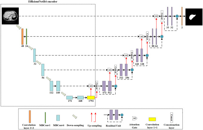
• Use a modified EfficientNet-B4 as the encoder to extract more feature information in the encoder stage.

• Add an attention gate to the original skip connection to eliminate irrelevant regions and focus on the liver area to be segmented.

• Employ the residual structure to replace the convolutional layer in the U-Net decoder and add a batch normalization layer to eliminate the gradient vanishment problem, accelerate the convergence speed, and achieve higher accuracy.

The structure of the paper is as follows: In the “Method” section, we describe the proposed EAR-U-Net framework in detail. Then, “Experiments” section provides the experimental results and discussion, and in the final “Conclusion” section, we summarize the whole work and give a future outlook.

Method

This section introduces the architecture of the proposed EAR-U-Net in detail. The proposed network EAR-U-Net consists of an encoder and decoder (Fig.  2). Considering the limitation of computing resources, we employ the modified EfficientNetB4 as the encoder. The encoder consists of nine stages, including a 3 × 3 convolutional layer, 32 mobile reversed bottleneck convolutional (MBConv) structures, and a 1 × 1 convolutional layer. The decoder is composed of five up-sampling and a series of convolution operations. The features extracted by the encoder are restored to the original image size, and then the segmentation results are obtained. To reduce the noise response and focus on specific features, we add an attention gate to the skip connection to make the segmented liver more accurate. The addition of the residual structure can increase the depth of the network. In the residual block, batch normalization (BN) and ReLU activation are performed after each convolution. The introduction of batch normalization can eliminate gradient diffusion and vanishment and accelerate the convergence of the network. Then we use ReLU to perform non-linear processing to improve the non-linear expression ability of the network.

Fig. 2.

The architecture of the proposed EAR-U-Net

The MBConv structure comprises a 1 × 1 convolution, a Depthwise convolution, a sequence-and-exception (SE) module, a 1 × 1 convolution for dimension reduction, and the dropout layer (Fig. 3). After the first 1 × 1 convolution and Depthwise Conv convolution, BN and Swish activation operations are conducted, and the second 1 × 1 convolution only performs BN operations. To fuse more feature information, we add a shortcut connection. The shortcut connection only exists when the shape of the feature matrix of the input MBConv structure is the same as that of the output feature matrix.

Fig. 3.

MBConv block

The SE module has dramatically improved the accuracy in image classification, target detection, and image segmentation. The SE module used in this paper (Fig. 4) consists of a global average pooling, two fully connected layers, and a Sigmoid activation function. In addition, the Swish activation function is added between the two full connection layers. Assuming input an image H × W × C, first, stretch it into 1 × 1 × C through the global pooling and fully connected layers, and then multiply it with the original image to give weight to each channel. In this way, the SE module enables the network to learn more liver-related feature information.

Fig. 4.

Squeeze and excitation block

Attention gate is a kind of attention mechanism that could automatically focus on the target area, suppress the response of irrelevant regions, and highlight the feature information crucial to a specific task, whose structure is shown in Fig. 5. First, g and x go through the 1 × 1 convolution operation in parallel and sum them up then perform the ReLU activation, 1 × 1 Conv and Sigmoid function operations sequentially, and resample to get the attention coefficient α. Finally, the attention coefficient α is multiplied by the input coding matrix x to obtain the final output.

Fig. 5.

Schematic of the attention gate (g is the decoding matrix, and x is the encoding matrix)

Experiments

This section first describes the datasets used in the paper, the image pre-processing, the dataset augmentation, and the implementation details. Then we provide the loss function and evaluation metrics of the evaluation. Finally, the experimental results are shown and analyzed, and the method’s limitation is discussed as well.

Experimental Setup

Image Dataset

In this experiment, we used the labeled training sets of the LiTS17² and SLiver07³ datasets for testing. The LiTS17-training dataset consists of 131 abdominal CT scans, with a large varying in-plane resolution from 0.55 to 1.0 mm and the inter-slice spacing from 0.45 to 6.0 mm. The number of slices ranges from 75 to 987. The size of each slice is 512 × 512. The SLiver07 training dataset consists of 20 CT scans, with in-plane resolution from 0.55 to 0.8 mm and inter-slice spacing from 1.0 to 3.0 mm. The number of slices ranges from 64 to 394, and each slice’s size is 512 × 512.

Image Preprocessing

We first set the Hounsfield intensity to (− 200, 200) to exclude irrelevant details and employ histogram equalization to enhance the contrast of the image. Then the CT image is down-sampled and resampled on the cross-section. Next, the spacings of the z-axis of all scans are adjusted to 1 mm to make the data more balanced. After that, we locate the slices with the liver and expand 20 slices outward to the edge slices at both ends. Finally, to save training time and reduce the memory requirements, we set each image’s size to 256 × 256.

Dataset Augmentation

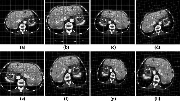
Considering the SLiver07-training dataset has a small amount of data, we enhanced the image data to improve the model’s generalization ability and prevent the overfitting problem. Meanwhile, we zoom the data with mirror flip, rigid and elastic deformations. Figure 6 illustrates some cases using different enhancement strategies.

Fig. 6.

Data augmentation. a Original CT with grid, b zoom, c mirror flip, d elastic deformation, e zoom and mirror flip, f zoom and elastic deformation, g mirror flip and elastic deformation, and h zoom, mirror flip, and elastic deformation

Implementation Details

We run all the experiments on a workstation with Ubuntu 18.04 operating system, graphics card RTX2080Ti, RAM 32G, single CPU Intel Xeon Silver 4110, and using the Pytorch1.8 deep learning framework for implementation. In the network training, we set the batch size to 16, set the epoch to 60, chose Adam as the optimizer, and set the learning rate to 0.001.

Loss Function Definition

The loss function makes an essential impact on the performance of CNN. In medical image segmentation, since ROI only covers a small area, and thus it is prone to lead to a sharp decline of the loss function to the local minimum during training, which may result in a significant segmentation deviation. However, cross-entropy [22] is able to measure the difference between two different probability distributions in the same random variable. The smaller the value of cross-entropy, the more accurate the prediction of the model. Therefore, cross-entropy can achieve good results in the segmentation network of pixel-level classification. The binary cross-entropy is defined in Eq. (1).

$$L_{\mathit{BCE}}\left(y,,,\widehat{y}\right)=-(ylog\left(\widehat{y}\right)+(1-y)log(1-\widehat{y}))$$ 1

where $y$ represents the actual value and $\widehat{y}$ represents the predicted result. Dice coefficient is one of the standard metrics to evaluate the segmentation effect. It can also be used to measure the distance between the segmentation result and the label [23]. As a loss function, Dice loss (DL) performs well in processing unbalanced datasets and can effectively reduce segmentation deviation caused by unbalanced ROI area and background. The DL used in this paper is defined in Eq. (2).

$$DL\left(y,,,\widehat{p}\right)=1-\frac{2y\widehat{p}+1}{y+\widehat{p}+1}$$ 2

where value 1 is added in numerator and denominator to ensure that the function is not undefined in edge case scenarios such as when $y=\widehat{p}=0$.

Evaluation Metrics

In this paper, we choose five commonly used metrics for evaluation, including Dice, volume overlap error (VOE), relative volume error (RVD), average symmetrical surface distance (ASSD), and maximum surface distance (MSD) [24].

Test on LiTS17-Training Dataset

In this section, we conducted experiments on the LiTS17-training dataset. We randomly selected 121 sets of scans as the training and validation sets, while the remaining ten sets as the test set. To verify EAR-U-Net’s performance, we first used the most commonly used DL as the loss function. Next, we performed comparative experiments and ablation experiments, respectively. Finally, to evaluate the effectiveness of DL + binary cross-entropy loss (BL), we select the combination of DL: BL = 1:1 as the loss function and take the classical models FCN [10], U-Net [11], attention U-Net [25], attention Res-U-Net, and EAR-U-Net for comparison.

Comparison with Classical Methods

First, we use DL as the loss function and compare the classic network FCN,⁴ U-Net,⁵ attention U-Net,⁶ and attention Res-U-Net.⁷ From Table 1, we can see that FCN results in the worst performance on Dice and VOE compared to the other four networks. On the other hand, compared with FCN, U-Net, attention U-Net, and attention Res-U-Net, the proposed EAR-U-Net model achieved the best performances on the four metrics (Dice, VOE, ASSD, and MSD) except for RVD. Specifically, its superiority on MSD is the most significant.

Table 1.

Quantitative results among the five methods on 10 LiTS17-training datasets

Method	Dice (%)	VOE (%)	RVD (%)	ASSD (mm)	MSD (mm)	Training time	Testing time
FCN	92.46 ± 3.52	13.83 ± 5.83	−1.65 ± 8.74	2.86 ± 1.24	81.94 ± 28.95	4 h 31 min 13 s	33 s
U-Net	94.08 ± 2.06	11.12 ± 3.65	−0.48 ± 5.58	3.07 ± 2.08	66.03 ± 27.91	7 h 49 min 13 s	36.4 s
Attention U-Net	94.37 ± 2.27	10.58 ± 4.04	0.37 ± 6.91	2.91 ± 1.57	82.03 ± 31.43	8 h 56 min 35 s	36.8 s
Attention Res-U-Net	94.93 ± 1.63	9.61 ± 2.97	2.23 ± 4.12	2.77 ± 1.69	62.69 ± 19.71	9 h 48 min 56 s	37.1 s
EAR-U-Net	95.95 ± 0.76	7.77 ± 1.42	0.50 ± 2.36	1.29 ± 0.35	35.96 ± 20.62	6 h 45 min 54 s	41.2 s

For each metric, bold value indicate the best result in that column

Therefore, EAR-U-Net enabled an improvement in the accuracy and stability of the segmentation. Besides, in terms of training time, EAR-U-Net is far less than U-Net, attention U-Net, and attention Res-U-Net, only more than FCN. However, in terms of test time, the EAR-U-Net is higher than other networks.

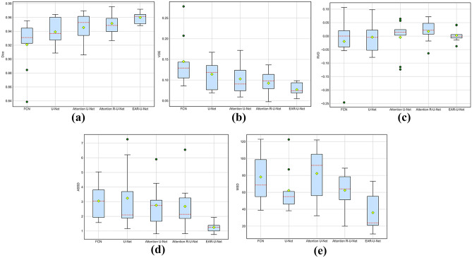
To demonstrate the robustness of the proposed EAR-U-Net more intuitively, we depict the boxplot on the five metrics. From Fig. 7, we can see that the proposed EAR-U-Net exhibits strong stability on all five metrics. Specifically, for Dice (Fig. 7a), the median of EAR-U-Net achieved the highest without outlier compared with the other four networks.

Fig. 7.

Comparative analysis on five metrics. a Dice, b VOE, c RVD, d ASSD, and e MSD

For VOE (Fig. 7b), the median of EAR-U-Net is the lowest, with the highest stability. Besides, the median on RVD (Fig. 7c) is closer to 0, but there are two outliers. Moreover, it shows extreme stability on ASSD (Fig. 7d), and the median of MSD (Fig. 7e) is far less than that of the other four networks.

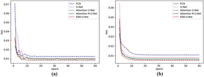
Figure 8 shows the loss curves of training and testing. From the figures, we can see that the loss value of the EAR-U-Net network is smoother and converges faster than other models.

Fig. 8.

Loss curves of different models on LiTS17 datasets. a The training set and b the validation set

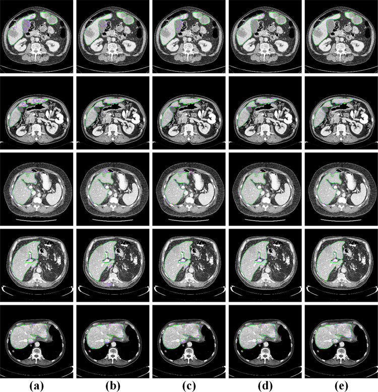
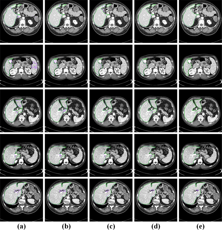
Figure 9 shows some visualizations of challenging cases. The first and the second row are discontinuous liver regions. (i) In the first row, FCN, U-Net, and the attention U-Net incorrectly segmented the gallbladder adjacent to the liver. Meanwhile, the attention Res-U-Net showed a little under-segmentation error. On the contrary, the proposed EAR-U-Net segmented the liver almost perfectly. (ii) In the second row, FCN showed obvious over-segmentation error, while other models performed well. (iii) The third row illustrates the segmentation of the liver with interlobar fissure. FCN and U-Net showed under-segmentation errors, but U-Net, attention Res-U-Net, and our proposed methods showed slight errors. (iv) The fourth row provided the liver area containing the portal vein. Again, we can see that FCN, U-Net, and attention U-Net have mistakenly under-segmented the portal artery. Nevertheless, the effect of attention Res-U-Net and our model is much superior to the other three models. (v) The fifth row shows the liver region containing the inferior vena cava. It can be seen that, except for the complete liver segmentation by the proposed network, the other four networks all mistakenly segment the inferior vena cava as the liver. The above demonstrates that our proposed network has advantages in the discontinuous liver region, the liver region with adjacent organs, and portal veins.

Fig. 9.

Visualization of challenging cases. a FCN, b U-Net, c attention U-Net, d attention Res-U-Net, and e EAR-U-Net (the green line represents the ground truth, and the purple line represents the segmentation result of the corresponding method)

Ablation Analysis on LiTS17-Training Datasets

To verify the optimality of the proposed network, we performed four comparative ablation experiments based on the efficient module (E-U-Net), efficient residual structures (ER-U-Net), and efficient attention gate (EA-U-Net). Specifically, we use the DL loss function for training, with the test results shown in Table 2.

Table 2.

Quantitative analysis results of ablation experiments

Method	Dice (%)	VOE (%)	RVD (%)	ASSD (mm)	MSD (mm)	Training time	Testing time
E-U-Net	95.23 ± 1.44	9.07 ± 2.62	0.10 ± 3.3	2.14 ± 1.21	80.34 ± 23.51	5 h 48 min 45 s	40.2 s
EA-U-Net	95.28 ± 1.37	8.99 ± 2.49	0.56 ± 2.94	2.11 ± 1.07	75.46 ± 21.71	6 h 27 min 27 s	40.9 s
ER-U-Net	95.62 ± 1.17	8.37 ± 2.15	0.78 ± 2.66	1.64 ± 0.49	68.41 ± 23.79	6 h 4 min 40 s	40.6 s
EAR-U-Net	95.95 ± 0.76	7.77 ± 1.42	0.50 ± 2.36	1.29 ± 0.35	35.96 ± 20.62	6 h 45 min 54 s	41.2 s

For each metric, bold value indicate the best result in that column

Table 2 shows that EAR-U-Net has achieved the best results on the five standard metrics except for RVD. The employment of residual structures enables a significant improvement on the Dice and ASSD. Furthermore, while the residual block and attention gate are both integrated into E-U-Net, the performances on all metrics improved significantly.

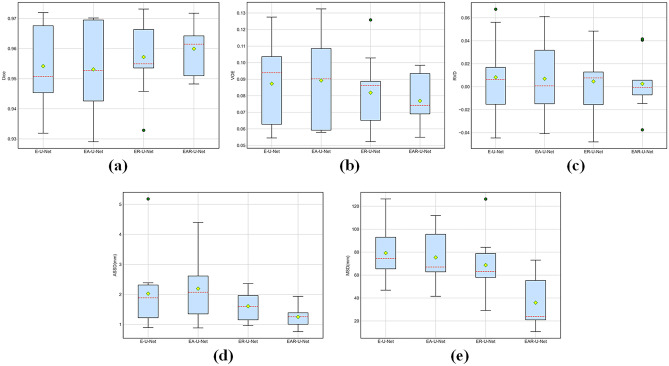
From the boxplot in Fig. 10, we can see that the method’s stability gradually improves with the superposition of the model. Compared with the other three networks, the proposed EAR-U-Net has improved on Dice, VOE, and ASSD (Fig. 10a, b, and d), and the performance improvement of MSD is the most significant (Fig. 10e). However, multiple outliers caused the proposed EAR-U-Net not to achieve the best performance in RVD. (Fig. 10c).

Fig. 10.

Comparative analysis on evaluation metrics. a Dice, b VOE, c RVD, d ASSD, and e MSD

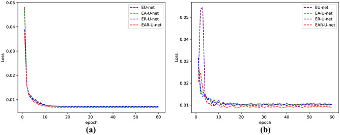
As for the running time, the network model’s training time and testing time increase with the overlay of modules. Nevertheless, such a trade-off way for segmentation accuracy is necessary for clinical application. Figure 11 shows the loss curves of different models. In the training and verification figures, with the superposition of modules, there is no significant difference between training and verification loss after stabilization, especially the training loss curve almost overlaps.

Fig. 11.

Loss curves of different models in LiTS17 datasets. a The training set and b the validation set

Evaluation of Different Loss Functions

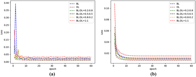
The loss function is crucial for the training of the model. Both DL and BL perform well in segmentation. In this paper, we assigned DL and BL different weights to train the models in LiTS17-training datasets. The experimental results listed in Table 3 show that the use of DL performs well on MSD, and the use of BL achieves the best results on RVD. However, given DL and BL a ratio of 1:1, the results show the best performance on Dice, VOE, and ASSD. In terms of training and test time, the impact of loss functions with different weights is slight and negligible. The result analysis of loss functions with different weights is shown in Fig. 12.

Table 3.

Result analysis of different weight loss functions using the EAR-U-Net model

Loss	Ratio	Dice (%)	VOE (%)	RVD (%)	ASSD (mm)	MSD (mm)	Training time	Test time
BL	1	96.07 ± 1.06	7.55 ± 1.96	0.44 ± 2.14	1.47 ± 0.67	48.28 ± 27.72	6 h 42 min 48 s	41.8 s
DL	1	95.95 ± 0.76	7.77 ± 1.42	0.5 ± 2.36	1.35 ± 0.82	35.96 ± 20.62	6 h 45 min 54 s	41.2 s
BL:DL	0.2:0.8	95.84 ± 1.10	7.96 ± 2.03	1.66 ± 3.08	1.67 ± 1.00	38.32 ± 14.86	6 h 51 min 7 s	44.2 s
BL:DL	0.5:0.5	96.13 ± 0.95	7.43 ± 1.75	1.29 ± 1.98	1.67 ± 0.86	43.84 ± 25.54	6 h 48 min 6 s	43.7 s
BL:DL	0.8:0.2	96.43 ± 0.90	6.88 ± 1.69	1.93 ± 2.42	1.42 ± 0.72	58.03 ± 33.99	6 h 52 min 45 s	43.6 s
BL:DL	1:1	96.63 ± 0.82	6.50 ± 1.52	1.18 ± 2.27	1.29 ± 0.35	36.79 ± 13.24	6 h 49 min 55 s	42.3 s

For each metric, bold value indicate the best result in that column

Fig. 12.

Loss curves of different loss functions on LiTS17 datasets. a Training set and b validation set

To verify the segmentation effect of the loss function combined with DL and BL in liver segmentation, we used the weight of DL: BL = 1:1 to test FCN, U-Net, attention U-Net, and attention Res-U-Net, respectively, and compared them with DL.

Table 4 lists the quantitative analysis results of the five models using DL + BL and DL. It can be seen that, compared with the single DL, using DL + BL has improved significantly on Dice, VOE, and ASSD. Specifically, the Dice scores of FCN, U-Net, atention U-Net, attention Res-U-Net, and our EAR-U-Net increased by 1.83%, 1.63%, 1.47%, 1.11%, and 0.68%, respectively.

Table 4.

Comparative results of different loss functions with four state-of-the-art methods on 10 LiTS17-training datasets

Methods	Loss	Dice (%)	VOE (%)	RVD (%)	ASSD (mm)	MSD (mm)	Training time	Test time
FCN	DL	92.46 ± 3.52	13.83 ± 5.83	−1.65 ± 8.74	2.86 ± 1.24	81.94 ± 28.95	4 h 31 min 13 s	33 s
	DL + BL	94.29 ± 1.9	10.75 ± 3.36	2.24 ± 5.02	2.69 ± 1.16	66.36 ± 33.46	4 h 36 min 22 s	33.4 s
U-Net	DL	94.08 ± 2.06	11.12 ± 3.65	−0.48 ± 5.58	3.07 ± 2.08	66.03 ± 27.91	7 h 49 min 13 s	36.4 s
	DL + BL	95.71 ± 2.10	8.16 ± 3.76	3.35 ± 4.22	2.06 ± 1.41	57.88 ± 29.03	7 h 50 min 27 s	36.9 s
Attention U-Net	DL	94.37 ± 2.27	10.58 ± 4.04	0.37 ± 6.91	2.91 ± 1.57	82.03 ± 31.43	8 h 56 min 35 s	36.8 s
	DL + BL	95.84 ± 1.29	7.96 ± 2.38	2.45 ± 2.81	2.03 ± 1.07	71.54 ± 34.06	8 h 58 min 15 s	36.8 s
Attention Res-U-Net	DL	94.93 ± 1.63	9.61 ± 2.97	2.23 ± 4.12	2.77 ± 1.69	62.69 ± 19.71	9 h 48 min 56 s	37.1 s
	DL + BL	96.04 ± 1.03	7.60 ± 1.90	0.86 ± 3.27	1.43 ± 0.47	56.99 ± 20.01	9 h 33 min 7 s	37.7 s
EAR-U-Net	DL	95.95 ± 0.76	7.77 ± 1.42	0.50 ± 2.36	1.35 ± 0.82	35.96 ± 20.62	6 h 45 min 54 s	41.2 s
	DL + BL	96.63 ± 0.82	6.50 ± 1.52	1.18 ± 2.27	1.29 ± 0.35	36.79 ± 13.24	6 h 49 min 55 s	42.3 s

For each metric, bold value indicate the best result in that column

In addition, compared with single DL, using DL: BL = 1:1 enables the standard deviation of all the compared methods on the five evaluation metrics to become smaller. Thus, it proves that the DL + BL loss function could improve the segmentation stability. As for training and testing time, the use of different loss functions did not produce significant differences.

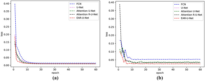
Figure 13 shows the loss in the train and validation using DL: BL = 1:1 for several classic models. The proposed EAR-U-Net converges the fastest for training loss (Fig. 13a), while FCN converges the slowest. For verification loss (Fig. 13b), both FCN and U-Net have relatively large volatility in the first few epochs. In contrast, EAR-U-Net has relatively tiny fluctuations, and the loss value is also minimized.

Fig. 13.

Loss curves of two-loss functions on LiTS17 datasets. a Loss in training set and b loss in the validation set

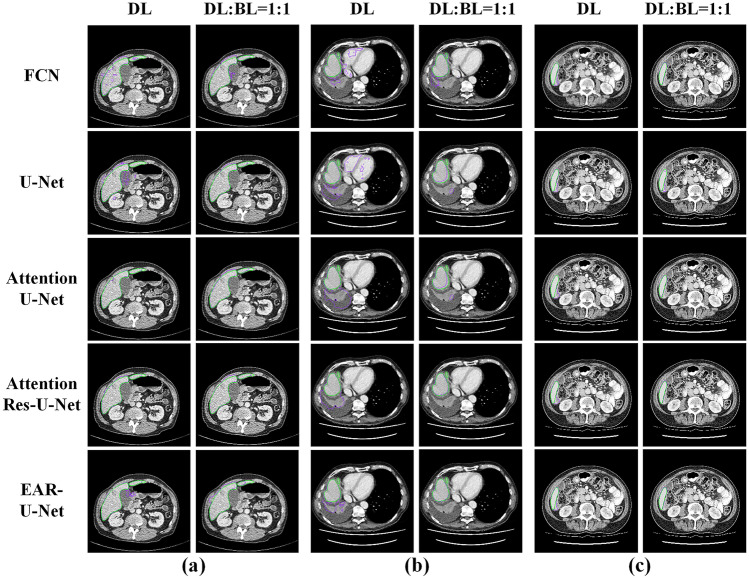
Figure 14 shows the visualization of partial segmentation results of FCN, U-Net, attention U-Net, attention Res-U-Net, and EAR-U-Net with DL and DL: BL = 1:1 as the loss function, respectively. Figure 14a shows the discontinuous liver region. When DL is used as the loss function, all methods showed over-/under-segmentation errors. In contrast, the errors by all methods are significantly alleviated when DL: BL = 1:1 is used as the loss function. Figure 14b demonstrates a case of a liver region with adjacent organs of low contrast. We found that the approach using DL as the loss function makes incorrect segmentation at several non-liver organs nearby. However, taking DL: BL = 1:1 as the loss function, only FCN results in noticeable under-segmentation, but the declinations of other models are all greatly improved. Specifically, our proposed EAR-U-Net almost entirely segmented the liver region. Figure 14c shows a typical case of a small liver region. When taking DL as the loss function, the five methods all showed under-segmentation errors, but the five models almost entirely segment the liver when taking DL: BL = 1:1 as the loss function.

Fig. 14.

Visualization of typical segmentation cases. a Discontinuous liver area, b liver area with the adjacent organs of low contrast, and c small liver area (green line stands for the ground truth, and the purple line represents the result of the corresponding method)

Comparisons of Different Segmentation Methods on LiTS17 Test Dataset

To further evaluate the performance of the proposed method, we participated in the MICCIA-LiTS17 challenge and compared it with some state-of-the-art methods. The challenge result is shown in Table 5 (our team’s name is hrbustWH402).

Table 5.

Comparison of various liver segmentation methods in LiTS17 test dataset

Method	Dimension	DC	DG	VOE	RVD	ASSD	MSD
Kaluva et al. [26]	2D	0.912	0.923	0.150	−0.008	6.465	45.928
Roth et al. [27]	2D	0.940	0.950	0.100	−0.050	1.890	32.710
Wardhana et al. [18]	2.5D	0.911	0.922	1.161	−0.046	3.433	50.064
Li et al. [19]	2.5D	0.961	0.965	0.074	−0.018	1.450	27.118
Jin et al. [17]	3D	0.961	0.963	0.074	0.002	1.214	26.948
Yuan [28]	3D	0.963	0.967	0.071	−0.010	1.104	23.847
Proposed method	2D	0.952	0.956	0.092	0.013	2.648	42.987

For each metric, bold value indicate the best result in that column

As can be seen from Table 5, in the MICCIA-LiTS17 challenge, our proposed method scored 0.952 (ranking 17) and 0.956 (ranking 15) on the two main evaluation metrics of Dice per case (DC) and Dice global (DG), respectively, which is superior to all the listed 2D-based networks. However, our performance is slightly inferior to 2.5D/3D-based networks since our proposed method does not use the 3D inter-slice information.

Test on SLiver07-Training Dataset

To verify the generalization capability of the proposed method, we used the weight of DL: BL = 1:1 as the loss function and conducted training and testing on the SLiver07-training dataset. We also compared it with the four classic networks of FCN, U-Net, attention U-Net, and attention Res-U-Net. As a result, the proposed EAR-U-Net achieved the best segmentation results in Dice, VOE, RVD, ASSD, and MSD. Specifically, the Dice reached 96.23% (as shown in Table 6).

Table 6.

Quantitative comparison with four state-of-the-art methods on Sliver07-training datasets

Methods	Dice (%)	VOE (%)	RVD (%)	ASSD (mm)	MSD (mm)	Training time	Test time
FCN	93.06 ± 1.21	12.96 ± 2.11	−4.47 ± 4.22	4.19 ± 2.81	114.82 ± 20.58	3 h 22 min 35 s	32.5 s
U-Net	95.09 ± 2.83	9.01 ± 4.96	1.51 ± 3.59	1.99 ± 0.87	97.62 ± 17.36	5 h 34 min 49 s	33 s
Attention U-Net	95.25 ± 3.14	8.94 ± 5.57	−2.21 ± 3.57	2.07 ± 1.63	99.85 ± 37.21	6 h 12 min 23 s	33.4
Attention Res-U-Net	95.72 ± 2.87	8.09 ± 5.11	−2.06 ± 6.6	1.81 ± 0.81	103.75 ± 16.56	6 h 58 min 56 s	33.4 s
EAR-U-Net	96.23 ± 2.65	7.16 ± 4.75	−1.42 ± 5.63	1.26 ± 0.68	87.32 ± 34.43	4 h 33 min 2 s	39.5 s

For each metric, bold value indicate the best result in that column

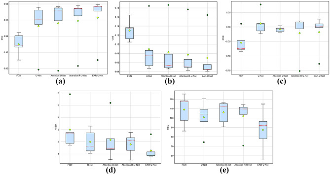
In addition, we also draw a box plot of all the evaluations in Fig. 15, which provides the Dice, VOE, RVD, ASSD, and MSD, respectively. The boxplot shows that EAR-U-Net results in the highest median on Dice, and the difference between the upper quartile and the lower quartile is the smallest. For the VOE, we can see that the median of EAR-U-Net is the smallest, while the median of FCN is the largest. For the RVD index, the median of EAR-U-Net is closer to 0. In terms of ASSD and MSD, the lowest median is also obtained by the proposed EAR-U-Net.

Fig. 15.

Comparative results of different methods on Sliver07-training datasets. a Dice, b VOE, c RVD, d ASSD, and e MSD

Moreover, the proposed EAR-U-NET also shows advantages in network training time. The training time is only 4 h 33 min 2 s, less than that of U-Net, attention U-Net, and attention Res-U-Net, but 26% more than FCN. However, the per-case test time is higher than that of other networks.

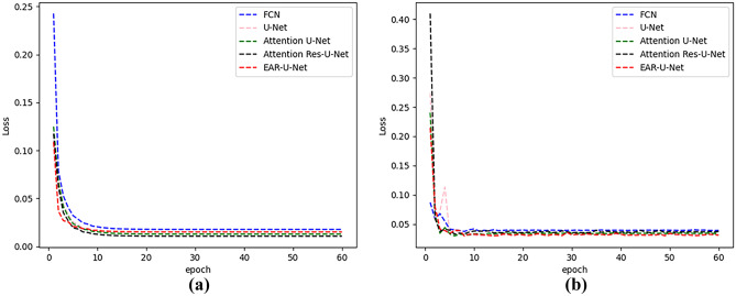
Figure 16 shows the loss curves of training and verification. EAR-U-Net converges the fastest and reduces to the lowest in the training loss. In the loss of verifying set, the loss values of the five networks all show some fluctuations in the first few epochs, but after the loss is stable, the value of EAR-U-Net is reduced to the lowest.

Fig. 16.

Loss curves of different models on SLiver07 datasets. a Training set and b validation set

Figure 17 shows some visualizations of hard-to-segment livers. (i) The first row is the result of liver segmentation of the gallbladder with similar contrast. It can be seen that FCN, U-Net, and attention U-Net have mistakenly segmented the gallbladder, while attention Res-U-Net and EAR-U-Net did not appear to have such an error. (ii) The liver in the second row is adjacent to the low-contrast gallbladder and spleen. It can be seen that FCN segmentation shows the worst effect, not only segmenting the gallbladder but also incorrectly segmenting the spleen far away from the liver. Meanwhile, U-Net also mistakenly segmented the gallbladder. Although the segmentation of attention U-Net and Res-U-Net have improved significantly, there are still some under-segmentation errors. Among all, the segmentation effect of EAR-U-Net is the best. (iii) The third row shows the discontinuous liver area. Again, both FCN and U-Net show obvious over-segmentation errors, while attention U-Net, attention Res-U-Net, and EAR-U-Net have alleviated the over-segmentation errors compared with FCN and U-Net. (iv) The fourth and fifth rows demonstrate the liver region containing portal veins. All methods result in specific over-segmentation errors, but the segmentation effect of EAR-U-Net on the portal vein is significantly improved compared to the other four networks. The above cases proved that our network has a better segmentation effect in the liver area containing adjacent organs and portal vein.

Fig. 17.

Test on tricky cases of SLiver07. a FCN, b U-Net, c attention U-Net, d attention Res-U-Net, and e EAR-U-Net (the green line denotes the ground truth, and the purple line indicates the segmentation result of the corresponding method)

Conclusion

This paper presents a new EAR-U-Net network for automatic liver segmentation in CT. To extract feature information more effectively, we employ EfficientNetB4 as the encoder. In addition, to highlight the feature information and eliminate the irrelevant feature responses, we add attention gates to the skip structure. Moreover, the introduction of the residual block also effectively prevents gradient vanishment.

In the experiments, we validated the proposed method on two publicly available datasets, LiTS17 and Sliver07. Specifically, we compared the proposed method with four classical models, including FCN, U-Net, attention U-Net, and attention ResU-Net. As a result, the proposed method achieved superior results on five standard metrics. Moreover, we also conducted experiments on different loss functions and proved that the combination of DL and BL produces a better effect in liver segmentation, including challenging cases. However, it is prone to false segmentation in the liver adjacent to other organs/tumors with low contrast.

In conclusion, the proposed EAR-U-Net could enrich the semantic information, enhance feature learning ability, and focus on small-scale liver information. Nevertheless, considering the limitations of the proposed EAR-U-Net in making full use of 3D data, we will focus on the 3D-based segmentation approach for the liver adjacent to organs/tumors with low contrast in future work.

Funding

This work is supported by the National Nature Science Foundation (no. 61741106).

Data Availability

Datasets are publicly available.

Code Availability

The code of the proposed EAR-U-Net is available at https://github.com/ZhangXY-123/Model/blob/master/EAR_Unet.py.

Declarations

Ethics Approval

Not applicable.

Consent to Participate

Not applicable.

Consent for Publication

Not applicable.

Conflict of Interest

The authors declare no competing interests.

References

- 1.Siegel R L, Miller K D, Jemal A . Cancer statistics, 2020[J]. CA: A Cancer Journal for Clinicians, 2020, 70(1). [DOI] [PubMed]
- 2.Gambino O, Vitabile S, Re G L, Tona G L, Librizzi S, Pirrone R, Ardizzone E, Midiri M. Automatic volumetric liver segmentation using texture based region growing[C]//2010 International Conference on Complex, Intelligent and Software Intensive Systems. IEEE, 2010: 146–152.
- 3.Seo K S. Improved fully automatic liver segmentation using histogram tail threshold algorithms[C]//International Conference on Computational Science. Springer, Berlin, Heidelberg, 2005: 822–825.
- 4.Li C, Wang X, Eberl S, Fulham M, Yong Y, Chen J. A likelihood and local constraint level set model for liver tumor segmentation from CT volumes[J] IEEE Transactions on Biomedical Engineering. 2013;60(10):2967–2977. doi: 10.1109/TBME.2013.2267212. [DOI] [PubMed] [Google Scholar]
- 5.Shi C, Cheng Y, Wang J, Wang Y, Mori K, Tamura S. Low-rank and sparse decomposition based shape model and probabilistic atlas for automatic pathological organ segmentation [J] Medical image analysis. 2017;38:30–49. doi: 10.1016/j.media.2017.02.008. [DOI] [PubMed] [Google Scholar]
- 6.Le T N, Huynh H T. Liver tumor segmentation from MR images using 3D fast marching algorithm and single hidden layer feedforward neural network[J]. BioMed research international, 2016, 2016. [DOI] [PMC free article] [PubMed]
- 7.Singh I, Gupta N. An improved K-means clustering method for liver segmentation[J]. International Journal of Engineering Research & Technology (IJERT), 2015: 235–239.
- 8.Krizhevsky A, Sutskever I, Hinton GE. Imagenet classification with deep convolutional neural networks[J] Advances in neural information processing systems. 2012;25:1097–1105. [Google Scholar]
- 9.He K, Zhang X, Ren S, Sun J. Deep residual learning for image recognition[C]//Proceedings of the IEEE conference on computer vision and pattern recognition. 2016: 770–778.
- 10.Long J, Shelhamer E, Darrell T. Fully Convolutional Networks for Semantic Segmentation[J] IEEE Transactions on Pattern Analysis and Machine Intelligence. 2015;39(4):640–651. doi: 10.1109/TPAMI.2016.2572683. [DOI] [PubMed] [Google Scholar]
- 11.Ronneberger O, Fischer P, Brox T. U-net: Convolutional networks for biomedical image segmentation[C]//International Conference on Medical image computing and computer-assisted intervention. Springer, Cham, 2015: 234–241.
- 12.Zhou Z, Siddiquee M, Tajbakhsh N, Liang J. Unet++: A nested u-net architecture for medical analysis and multimodal learning for clinical decision support image segmentation[M]//Deep learning in medical image analysis and multimodal learning for clinical decision support. Cham: Springer; 2018. pp. 3–11. [DOI] [PMC free article] [PubMed] [Google Scholar]
- 13.Budak Ü, Guo Y, Tanyildizi E, Şengür A. Cascaded deep convolutional encoder-decoder neural networks for efficient liver tumor segmentation[J] Medical hypotheses. 2020;134:109431. doi: 10.1016/j.mehy.2019.109431. [DOI] [PubMed] [Google Scholar]
- 14.Ben-Cohen A, Diamant I, Klang E, Amitai M, Greenspan H. Fully convolutional network for liver segmentation and lesions detection[M]//Deep learning and data labeling for medical applications. Cham: Springer; 2016. pp. 77–85. [Google Scholar]
- 15.Sun C, Guo S, Zhang H, Li J, Chen M, Ma S, Jin L, Liu X, Li X, Qian X. Automatic segmentation of liver tumors from multi-phase contrast-enhanced CT images based on FCNs[J] Artificial intelligence in medicine. 2017;83:58–66. doi: 10.1016/j.artmed.2017.03.008. [DOI] [PubMed] [Google Scholar]
- 16.Zhang Y, He Z, Cheng Z, Yang Z, Shi Z. Fully convolutional neural network with post-processing methods for automatic liver segmentation from CT[C]//2017 Chinese Automation Congress (CAC). IEEE, 2017: 3864–3869.
- 17.Jin Q, Meng Z, Sun C, Wei L, Su R. RA-UNet: A hybrid deep attention-aware network to extract liver and tumor in CT scans[J] Frontiers in Bioengineering and Biotechnology. 2020;8:1471. doi: 10.3389/fbioe.2020.605132. [DOI] [PMC free article] [PubMed] [Google Scholar]
- 18.Wardhana G, Naghibi H, Sirmacek B, Abayazid M. Toward reliable automatic liver and tumor segmentation using convolutional neural network based on 2.5 D models[J] International journal of computer assisted radiology and surgery. 2021;16(1):41–51. doi: 10.1007/s11548-020-02292-y. [DOI] [PMC free article] [PubMed] [Google Scholar]
- 19.Li X, Chen H, Qi X, Dou Q, Fu CW, Heng PA. H-DenseUNet: hybrid densely connected UNet for liver and tumor segmentation from CT volumes[J] IEEE transactions on medical imaging. 2018;37(12):2663–2674. doi: 10.1109/TMI.2018.2845918. [DOI] [PubMed] [Google Scholar]
- 20.Lei T, Wang R, Zhang Y, Wan Y, Nandi A K. Defed-net: Deformable encoder-decoder network for liver and liver tumor segmentation[J]. IEEE Transactions on Radiation and Plasma Medical Sciences, 2021.
- 21.Tummala B M, Barpanda S S. Liver tumor segmentation from computed tomography images using multi-scale residual dilated encoder‐decoder network[J]. International Journal of Imaging Systems and Technology, 2021.
- 22.Ma Y D, Liu Q , Qian Z B. Automated image segmentation using improved PCNN model based on cross-entropy[C]// Proceedings of 2004 International Symposium on Intelligent Multimedia, Video and Speech Processing, 2004. IEEE, 2005.
- 23.Sudre C H, Li W, Vercauteren T, Ourselin, Sébastien, Cardoso M J. Generalised dice overlap as a deep learning loss function for highly unbalanced segmentations[M]//Deep learning in medical image analysis and multimodal learning for clinical decision support. Springer, Cham, 2017: 240–248. [DOI] [PMC free article] [PubMed]
- 24.Heimann T, Ginneken BV, Styner MA, et al. Comparison and evaluation of methods for liver segmentation from CT datasets[J] IEEE transactions on medical imaging. 2009;28(8):1251–1265. doi: 10.1109/TMI.2009.2013851. [DOI] [PubMed] [Google Scholar]
- 25.Oktay O, Schlemper J, Folgoc L L, Lee M, Heinrich M, Misawa K, Mori K, Mcdonagh S, Hammerla NY, Kainz B. Attention u-net: Learning where to look for the pancreas[J]. arXiv preprint arXiv:1804.03999, 2018.
- 26.Kaluva K C, Khened M, Kori A, Krishnamurthi G. 2D-densely connected convolution neural networks for automatic liver and tumor segmentation[J]. arXiv preprint arXiv:1802.02182, 2018.
- 27.Roth K, Konopczyński T, Hesser J. Liver lesion segmentation with slice-wise 2d tiramisu and tversky loss function[J]. arXiv preprint arXiv:1905.03639, 2019.
- 28.Yuan Y. Hierarchical convolutional-deconvolutional neural networks for automatic liver and tumor segmentation[J]. arXiv preprint arXiv:1710.04540, 2017.
Associated Data
This section collects any data citations, data availability statements, or supplementary materials included in this article.
Data Availability Statement