Regional Personality Assessment through Social Media Language

Abstract

Objective:

We explore the personality of counties as assessed through linguistic patterns on social media. Such studies were previously limited by the cost and feasibility of large-scale surveys; however, language-based computational models applied to large social media datasets now allow for large-scale personality assessment.

Method:

We applied a language-based assessment of the five factor model of personality to 6,064,267 U.S. Twitter users. We aggregated the Twitter-based personality scores to 2,041 counties and compared to political, economic, social, and health outcomes measured through surveys and by government agencies.

Results:

There was significant personality variation across counties. Openness to experience was higher on the coasts, conscientiousness was uniformly spread, extraversion was higher in southern states, agreeableness was higher in western states, and emotional stability was highest in the south.

Across 13 outcomes, language-based personality estimates replicated patterns that have been observed in individual-level and geographic studies. This includes higher Republican vote share in less agreeable counties and increased life satisfaction in more conscientious counties.

Conclusions:

Results suggest that regions vary in their personality and that these differences can be studied through computational linguistic analysis of social media. Furthermore, these methods may be used to explore other psychological constructs across geographies.

Just as geographic regions vary in climate and culture, communities within these regions can systematically vary in their psychological characteristics. However, researching geographical psychological variation with traditional self-reported methods is expensive and time-consuming, and current studies of regional variation in the U.S. are limited to a few select datasets. The recent proliferation of public, geotagged data in social media offers new opportunities for researchers interested in regional differences. In the present study, we describe and evaluate a method for estimating regional personality differences through language, using publicly available data from Twitter.

Regional Variation in Personality

While research on regional variation in personality dates back to the 1970s (Krug & Kulhavy, 1973), web-based data collection has recently enabled studies at a much larger scale. To date, researchers have collected millions of self-reported measures of personality dimensions across and within several countries (e.g., Elleman et al., 2018; Rentfrow et al., 2013). These studies have typically centered on three questions: (1) Do regions reliably differ in their distribution of psychological traits?, (2) How are these differences related to important regional outcomes, such as political, economic, social, and health behaviors?, and (3) How do these differences come about?

Over the two decades, researchers have identified reliable psychological differences between geographic regions, while gradually increasing the spatial resolution of their analyses. Earlier work examined differences between nations (e.g., Allik & McCrae, 2004; McCrae et al., 2005), but research soon expanded to within-nation analyses, such as comparisons of large multi-state regions (Rogers & Wood, 2010) and individual states in the U.S. (e.g., Obschonka et al., 2013; Park et al., 2006; Rentfrow et al., 2008, 2009, 2010, 2013). More recently, researchers have leveraged large datasets of self-reported measures to estimate differences at much smaller regions: zip codes (Bleidorn et al., 2016; Ebert et al., 2019; Elleman et al., 2020) and Metropolitan Statistical Areas (MSAs; Obschonka et. al, 2016) in the U.S., Local Authority Districts in the United Kingdom (Rentfrow et al., 2015), administrative regions and labor market regions in Germany (Ebert et al., 2019), metropolitan areas of London (Jokela et al., 2015), and continental cities in China (Wei et al., 2017).

The majority of studies have focused on average differences across broad personality dimensions, specifically the Big Five: extraversion, agreeableness, conscientiousness, emotional stability (or neuroticism, reversed) and openness to experience (Costa & McCrae, 1992; John & Srivastava, 1999). Whether measured through traditional self-report questionnaires (e.g., Rentfrow et al., 2008) or by studying regional stereotypes (e.g., McCrae et al., 2005; Rogers & Wood, 2010), personality dimensions tend to vary between regions in reliable ways. For example, studies of the contiguous U.S. consistently find that the country’s coastal regions are higher in openness to experience, while the country’s center tends to be less open and more conventional (Rentfrow et al., 2008; Rentfrow et al., 2013; Rogers & Wood, 2010).

Regional personality differences are not only reliably indicated across studies and approaches, but they correlate with a wide range of political, economic, social, and health (PESH) outcomes in face valid ways (Rentfrow et al., 2013; Rentfrow & Jokela, 2016). The patterns of these regional correlations are generally consistent with those seen at the individual level. In more open regions, for example, PESH outcomes at the regional level align with behaviors exhibited by more open individuals, including more liberal voting patterns, greater acceptance of unconventional values, and more people working in artistic and creative occupations. Similarly, more emotionally stable areas tend to have better health and greater longevity, consistent with the patterns seen with emotional stability at the individual level (Ozer & Benet-Martinez, 2006; Roberts et al., 2007).

Rentfrow et al. (2016) proposed that regional psychological variation, including personality differences, emerge through three distinct processes: social influence, ecological influence, and selective migration. Social influence refers to the process through which local culture and customs gradually shape broader social norms, which then influence the thoughts, feelings, and behaviors of individuals. Ecological influence describes the effects of the local physical environment, including geographic features (e.g., heat, altitude, access to resources) and the impact of those features on disease risk, stress, and survivability. Selective migration suggests that certain environments (e.g., bustling cities) are inherently more attractive to some personalities (e.g., excitement-seeking or highly sociable) or some personalities are more open to the prospect of moving to new places, thus impacting migration patterns.

Challenges to Regional Measurement

The most common approach to estimating regional personality differences is to aggregate, usually by averaging, the self-reported scale scores from all individuals within a given region. The resulting averages are then compared across regions and with other indicators of interest within those regions (e.g., voting patterns, mortality rates). This approach brings at least three types of methodological challenges worth noting: cost of large-scale data collection, potential response biases found in aggregated self-reports, and the spatial dependencies within the data.

First, the sheer scale of data collection required to adequately sample a wide geographic area, like the U.S., creates a steep barrier to researchers interested in regional differences. While there are a handful of relevant datasets with observations mapped to U.S. states (e.g., Elleman et al., 2018; Park et al., 2006), several of these datasets cannot be used for analysis of sub-state regions, such as MSAs or counties, because they lack the necessary sample size or the necessary geographic information. All sub-state analyses of U.S. regions have drawn from one of a few large internet-based collections of self-reported personality measures, such as the Gosling-Potter Internet Personality Project (GPIPP; Gosling et al., 2004) or the Synthetic Aperture Personality Assessment project (SAPA; Condon et al., 2017). These massive datasets required several years of data collection to reach a sample size sufficient for geographic analyses as fine-grained as counties.

Secondly, with a few exceptions, analyses of regional personality are based on self-reports, which may introduce unusual response biases when aggregated and compared across regions. For example, Wood and Rogers (2011) noted high similarities between aggregated self-reports and regional stereotypes for some Big Five dimensions (e.g., openness and neuroticism) but substantial differences between these two estimates of regional conscientiousness. When compared to regional indicators, aggregated self-reports of conscientiousness also yield several counterintuitive associations, such that higher conscientiousness is associated with lower income and wealth (Elleman et al., 2020; Rentfrow et al., 2008, 2013), poorer health (Rentfrow et al., 2013), more heart disease deaths (Elleman et al., 2018), higher mortality (Rentfrow et al., 2008), and more violent crimes (Elleman et al., 2018). These counterintuitive associations with conscientiousness at the regional level appear across several studies, at different levels of analysis (i.e., U.S. states and U.S. counties), and are all in the opposite direction of the associations observed with conscientiousness the individual level (Ozer & Benet-Martinez, 2006; Roberts et al, 2014).

One contributing factor to these unexpected associations may be the reference-group effect (RGE; Heine, Lehman, Peng, & Greenholtz, 2002). Responses to self-report items are, in part, made by comparing one’s self to others in the surrounding area. For example, a highly conscientious person surrounded by exceptionally conscientious people may underestimate his/her own conscientiousness, despite being highly conscientious by objective standards. Likewise, overestimation would occur when that person is surrounded by highly unconscientious people. Because less conscientious groups tend to overestimate and highly conscientious groups tend to underestimate, RGE errors can systematically inflate or depress regional averages, potentially creating the counterintuitive correlations found across several regional analyses. While RGE errors have been suggested as explanations for counterintuitive associations with conscientiousness at the regional level, it is not clear why only conscientiousness would be susceptible to such effects (Wood and Rogers, 2011). Indeed, Youyou et al. (2017) suggested that self-report of all five factors have RGE by demonstrating that scores within social diads (romantic partners, close friends) diverge significantly more when measures from self-report than from behavior-based assessments. Such measure-level effects could aggregate to different biases at the regional level and therefore using a language-based assessment regionally can provide evidence toward where self-report effects might bias regional aggregates.

Heine et al. (2008) found that these inconsistencies can be resolved when regional conscientiousness is measured by aggregated behavioral criteria (e.g., postal worker speed, walking speed, and the accuracy of public clocks; Levine & Norenzayan, 1999) or regional stereotypes (e.g., aggregate ratings of a region’s conscientiousness from individuals living outside of that region). These alternative measurements are positively correlated with regional Gross Domestic Product (GDP) and longevity, while aggregated self-reports are negatively correlated with the same indicators. While behavior-based measures of conscientiousness may avoid potential biases in self-reports, collecting behavioral data at the scale needed for high-resolution geographical analysis has not been practical. Furthermore, behaviors related to less visible traits, such as emotional stability, may be more difficult to measure by publicly available, behavioral cues (Vazire & Carlson, 2011).

In addition to behavior-based measures, informant-reports are also known to alleviate some, but not all, of the biases associated with self-report. Despite this, several national level studies have shown informant-report measures are consistent with self-report. Drawing from a large sample of informant-reports across 36 countries, Gebauer et al. (2016) replicated evidence for cross-cultural differences in the relationship between religiosity and psychological adjustment. Notably, relationships between religiosity, self-esteem, and both conscientiousness and agreeableness remain consistent when measured with both informant- and self-reports, thus, dispelling prior alternative explanations to the religiosity-psychological adjustment relationships, which included self-report biases. In a similar large cross-cultural study, Entringer et al. (2021) showed that relationships between Big Five facets and religiosity hold when measured with both self and informant reports.

Lastly, analyses of regional differences must account for spatial dependencies, or the fact that the similarities or differences between two regions are related to their physical distance from each other (Tobler, 1970). Several of the variables studied in this area exhibit spatial autocorrelation, such that the attributes of two regions are more similar as they are closer to each other. These underlying dependencies between units in spatial data violate the independence assumptions of standard ordinary least squares (OLS) techniques, potentially leading to inflated Type I errors (Greene, 2000). Estimators such as Moran’s I can indicate the presence and degree of spatial autocorrelation among observations, suggesting that OLS methods would be inappropriate (Moran, 1950). In these cases, analytic techniques such as multilevel modeling or spatially lagged regression modeling, which directly incorporate neighboring observations, may be required to account for the spatial dependence and produce valid estimates (Arbia, 2014).

The current study attempts to address these challenges by using a language-based assessment method that leverages the vast amount of language publicly available from Twitter. This method starts with individual-level models originally trained (and validated) to predict psychological attributes of single individuals based on their language use and adapts them to the aggregated language of large groups. This method does not require self-report measures at the group level, removing the cost of collecting such data at large scale and avoiding potential biases introduced by aggregating self-reports. To validate these language-based estimates, we compare them to other relevant political, economic, social, and health variables collected at the same level, using regression techniques appropriate for spatial data.

Social Media Language as a Personality Measure

Many studies have identified language as a reliable source of personality cues (e.g., Kern et al., 2014; Pennebaker & King, 1999; Pennebaker, Mehl, & Niederhoffer, 2003; Tausczik & Pennebaker, 2010; Schwartz et al., 2013b; Yarkoni, 2010). Regional language may be a valuable source of behavioral data for studying personality. A major advantage to using language is the sheer size of available data. Social media platforms, such as Facebook and Twitter, generate hundreds of millions of messages every day, and many of these messages can be geolocated (i.e., tied back to their originating location with high precision). Social media messages are particularly useful for studying personality, as many users rely on these platforms to share their own thoughts, feelings, activities, and plans (Naaman, Boase, & Lai, 2010). Although impression management does occur, research by Back et al. (2010) demonstrates that users’ self-presentations in social media are generally consistent with their actual personality traits and not simply idealized versions of themselves.

Methods developed in computer science fields can further refine the analysis of social media language for personality research. These methods, including topic modeling (Atkins et al., 2012; Blei, Ng, & Jordan, 2003), can extract features from language that are less sensitive to word sense ambiguity, neologisms, or misspellings than handcrafted dictionaries.

When combined with predictive modeling techniques from machine learning, the language features extracted from social media data can create valid and reliable measures of Big Five personality dimensions. For example, Park et al. (2015) found that predictions of Big Five dimensions based on social media language models converged with self-report and informant-report measures of the same dimensions. These language-based estimates also correlated with external criteria as theoretically expected and were stable over time, as shown by test-retest correlations over six-month periods. Similar language-based models can be applied to social media language within geographic regions, using the aggregated individual-level predictions to estimate regional differences.

While the characteristics of social media differ from the general population in some ways (Perrin & Anderson, 2019), the regional differences in social media language are still useful for studying representative outcomes from those regions. For example, models based on Twitter language can predict a wide range of U.S. county-level outcomes, including obesity and diabetes rates (Pearson r = 0.43 and 0.35, respectively; Culotta, 2014), heart disease mortality (r = 0.42; Eichstaedt et al., 2015), life satisfaction (r = 0.55; Giorgi et al., 2019), excessive drinking (r = 0.65; Curtis et al., 2018), and entrepreneurial activity (r = 0.45; Obschonka et al., 2019). Of note, these studies demonstrate empirically that despite all potential biases, social media language contains sufficient and systematic outcome-related variance to predict these government or Centers of Disease Control and Prevention reported outcomes at the stated prediction accuracies out-of-sample. Specifically, while Twitter users are only a subset of the local population, if this subset is unrepresentative in consistent ways across regions—e.g., Twitter users tend to be younger and more affluent (PEW, 2019)—then covariation between Twitter language and representative outcomes will be noisier but still useful for predictive models. It is thus important, as we do here, to validate social media based models against outcomes assessed through other means and accepted to be representative of their populations (Kern et al., 2016).

The Present Study

The primary goal of this study was to explore the utility of language-based assessment for studying aggregate personality characteristics of U.S. counties¹. The study was guided by two questions: (1) Can regional personality differences in the U.S. be detected through social media language, such as Twitter?, (2) Are the differences found from language-based estimates related to political, economic, social, and health (PESH) outcomes?

Because we are using a novel method, our analyses were descriptive and exploratory rather than confirmatory. We visualized personality scores through county-level maps of the U.S. to depict each county relative to others in the US and be able to examine regional trends. We then tested reliability and convergent validity of the language-based estimates, comparing the estimates to self-report based scores at both the county and state levels, using multiple data sources. Further, if language-based estimates are capturing true differences in regional personality, they should be associated with relevant outcomes in PESH domains. We compared our personality correlates of PESH outcomes with prior individual- and county-level research to further validate our personality estimates.

Following Rentfrow et al. (2008), we drew on a comprehensive review by Ozer and Benet-Martinez (2006) and meta-analyses by Roberts et al. (2007), which together summarize links between personality and criminality, religiosity, academic and occupational success, social attitudes, and health/longevity. In addition, we used DeNeve and Cooper’s (1998) meta-analysis of personality and subjective well-being to inform predictions about county-level well-being and mental health.

To aid comparisons to prior work, we also selected several PESH indicators from recent analyses. At the state level, Elleman et al. (2018) compared patterns of correlations between Big Five dimensions and several PESH outcomes, including voting outcomes, occupational and industrial differences, education, marriage rates, crimes rates, and patenting rates. Ebert et al. (2019) included several similar PESH indicators in an analysis of U.S. counties. With a few exceptions, both studies reported several significant correlations between a region’s average self-reported personality dimensions and PESH indicators, in directions that aligned with expectations from individual-level findings. We replicate this procedure, using language-based estimates of personality in place of aggregated self-reports.

We also aimed to produce an open-source county-level personality database for researchers in this area. To this end, we are releasing language-based 5 factor personality estimates for all 2,041 counties which meet our data integrity thresholds². We believe such a dataset will be useful across a number of fields, including psychology, public health, politics, and economics.

Predicted associations between PESH indicators and county-level personality.

Openness predictions.

Openness has been consistently linked to more liberal political values, unconventional beliefs, and artistic and intellectual interests (Jost et al., 2003; McCrae, 1996; Ozer & Benet-Martinez, 2006). State-level (Rentfrow et. al, 2013, Elleman et al., 2018) and county-level analyses (Ebert et al., 2019) have found that regional openness correlated with votes for liberal political candidates, higher educational attainment, and higher proportions of the local population working in arts and entertainment. Therefore, we predicted county-level openness to be correlated with high votes for liberal presidential candidates in 2012 and 2016, higher proportions of individuals with a college degree, and relatively more individuals working in the arts and entertainment industries.

Conscientiousness predictions.

Conscientiousness is linked to greater educational and occupational success, lower substance use, and better health and longevity (Bogg & Roberts, 2013; Kern & Friedman, 2008; Kern, Friedman, Martin, Reynolds, & Luong, 2009; Lodi-Smith et al., 2010; Roberts et al., 2007; Roberts, Lejuez, Krueger, Richards, & Hill, 2014). In addition, DeNeve and Cooper’s (1998) meta-analysis on well-being found that conscientiousness was the strongest positive predictor of life satisfaction. However, as described above, geographic analyses, based on aggregated self-reports, have reported several counterintuitive associations between conscientiousness and regional indicators. For example, state-level analyses across seven samples found conscientiousness correlated with lower well-being, higher violent and property crime, higher heart disease deaths (Elleman et al., 2018). At lower levels of analysis, findings are mixed. In a ZIP code-level analysis, Elleman et al. (2020) reported a negative correlation (r = −.11, p < .05) between conscientiousness and median income. A county-level analysis by Ebert et al. (2019) found no association with university degrees (r = −.02, ns) nor with life expectancy (r = .02, ns).

There are several explanations as to why individual and group level analyses disagree, we did not have a specific hypothesis about which explanation is correct.

Extraversion predictions.

Extraversion is associated with more positive emotions and greater social involvement, both of which correlated with better health outcomes and longevity (Ozer & Benet-Martinez, 2006; Pressman & Cohen, 2005; Roberts et al., 2007). County-level analyses (Ebert et al., 2019) have shown extraversion associated with lower mortality, university degrees, and lower violent crimes. Therefore, we expected county-level extraversion to correlate with higher levels of social support, life satisfaction, and education, as well as lower mortality.

Agreeableness predictions.

Agreeableness is linked to more stable social relationships, lower interpersonal conflict, lower mortality, and higher life satisfaction (DeNeve & Cooper, 1998; Ozer & Benet-Martinez, 2006; Roberts et al., 2007). Similar patterns have been found at the county-level: lower mortality and higher percentage married (Ebert et al., 2019). The same study also found increased agreeableness associated with a higher percentage of Republican votes in the 2008 and 2012 U.S. elections (r = .04, p < .05; for both elections). Therefore, we expected agreeableness to correlate with greater social support, lower violent crime rates, higher percentage Republican voting, and lower mortality.

Emotional stability predictions.

Greater emotional stability has been linked to better occupational outcomes, less interpersonal conflict, lower mortality, lower depression, and higher life satisfaction (DeNeve & Cooper, 1998; Ozer & Benet-Martinez, 2006; Roberts et al., 2007). Again, similar patterns have been found at the state and county-level, with higher emotional stability associated with lower mortality, higher education, lower trade, and higher proportions working in professional and managerial occupations (Elleman et al., 2018; Ebert et al., 2019). Therefore, we predicted that emotional stability would correlate with higher education attainment and income, lower crime rates, lower mortality, higher proportion of professional and managerial occupations, and higher subjective well-being.

Methods

Overview

Our approach to assessing personality at the county level builds on prior work which developed and validated language-based assessments of individuals’ personality dimensions (Park et al., 2015; Schwartz et al., 2013b). The overall approach can be understood in two phases, as illustrated in Figure 1: model development and model application. We utilize the language-based assessment model from Park et al., (2015). Park created the personality measures trained over 66,000 Facebook participants, producing five regression models, one for each Big Five dimension. Each regression model has thousands of language features (indicating usage of particular words and phrases) as predictors and generates an estimated personality dimension score for each individual. To orient the reader, we include the predictive accuracies (Pearson r) for each personality dimension as reported in Park et al. (2015): openness r = 0.46, conscientiousness r = 0.38, extraversion r = 0.41, agreeableness r = 0.40, and emotional stability r = 0.39.

Figure 1.

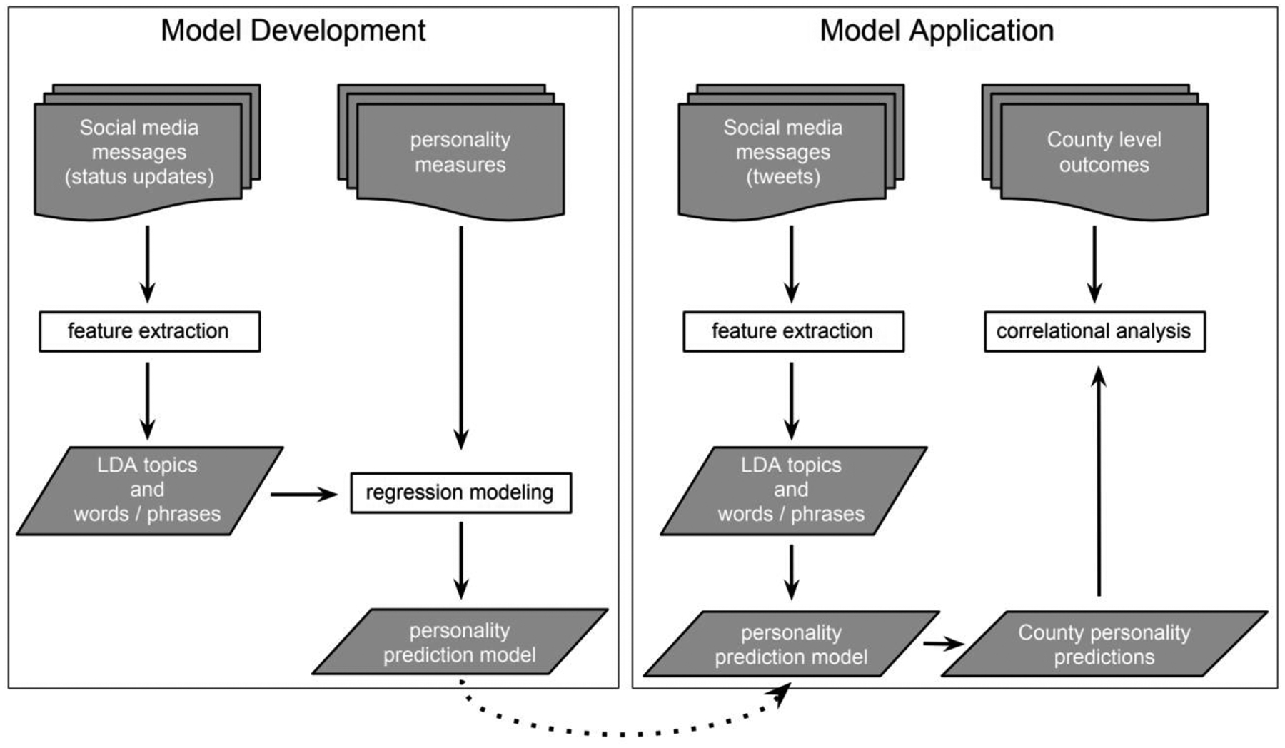
Process flow for developing predictive models and applying them to county-level language.

As detailed in the next section, we applied these models to the mean language patterns of 2,041 U.S. counties from the County Twitter Lexical Bank (Giorgi et al., 2018) -- spanning 6,064,267 users with a total of 1.5 billion messages -- to generate county-level Big Five dimension scores. As the language-based personality assessment models are linear, using the mean language patterns per county is mathematically equivalent to applying the personality model to every single user at a time, and then taking the mean per county. After exploring the geographic distribution of county-level personality, we then investigated their relationship with several representative measures of PESH outcomes through correlational analyses. This study followed the Strengthening the Reporting of Observational studies in Epidemiology (STROBE) guidelines (Von Elm et al., 2007).

Language Model Application

After training and evaluating five regression models (one for each trait) for the individual-level data, we used the same models to generate personality predictions at the county level.

Social media language features.

County-level language data was drawn from Twitter, a social networking platform on which users write short messages, or “tweets,” which are similar to Facebook status updates. Unlike Facebook messages, most tweets are publicly available. Specifically, we used the County Tweet Lexical Bank (Giorgi et al., 2018), which contains the mean mentions of approximately 24,000 word phrases as well as 2000 Latent Dirichlet Allocation (LDA; Blei, Ng, & Jordan, 2003) topics, or sets of semantically related words, automatically derived from a large corpus of Facebook statuses (Schwartz et al., 2013b). These features are available for 2,041 U.S. counties (Giorgi et al., 2018). This open-source aggregate dataset was built from a random 10% sample of tweets collected between July 2009 and April 2014, supplemented with another random 1% sample from May 2014 to February 2015 (Preotiuc-Pietro et al., 2012). Before producing the mean lexical features, tweets were filtered for English, using the Python package langid (Lui & Baldwin, 2012), and matched to their originating U.S. county, based on geotagged metadata or by using the self-reported location from each user’s profile using the methodology from Schwartz et al., (2013a). The final County Tweet Lexical Bank data was calculated from 6,064,267 users who posted at least 30 times and counties with 100 such users, resulting in 1.53 billion tweets across 2,041 counties. Based on data from the U.S. Census Bureau’s 2010 American Community Survey, over 96% of the U.S. population lives within the included counties. This provided, at the county level, the same word, phrase, and topic frequency variables as those needed as input to the pretrained language-based assessments (Park et al., 2015).

Domain adaptation.

Because the Big 5 language-based assessments were trained on source data of user-level Facebook language (Park et al., 2015), we applied a domain adaptation technique, Target Side Domain Adaptation (TSDA; Rieman et al., 2017), to adjust for differences in language use between that source (Facebook) and our target (county-level Twitter data). This method, which was specifically developed for adjusting models built on Facebook to county-level Twitter data (Rieman et al., 2017), applies two corrections: (1) adjusting the target side word frequencies to correct for outlier counties (i.e. areas that systematically use the word differently) and (2) adjusting for the different word distributions between Facebook and Twitter, removing outliers in the frequency distributions of word use. As an example of the first step, if “new” appears five times more often in counties near New York City as compared to overall word counts, then it is assumed to be used in a geographically-specific sense, ill-suited for the application of a general prediction model, and its value replaced by the global mean frequency for “new.” For the second step of TSDA, a ratio of each words’ difference in mean relative frequencies across the datasets divided by the sum of mean relative frequencies. When the ratio is greater than a threshold (ϵ = 0.80; Rieman et al., 2017), the word’s frequency is globally replaced with the mean Facebook frequency. For example, “retweet” appeared more often in the Twitter data than the Facebook data on which the personality models were trained, so it was adjusted (that is, effectively ignored by the model).

County-level personality estimation.

We applied the five language-based assessments (Park et al., 2015) to the county-level TSDA-adjusted word, phrase, and topic data, generating estimates of each Big Five trait for each county. To ease interpretation, we converted all county-level trait estimates to z scores―mean centered across the US and normalized by the standard deviation across US counties.

Reliability of County Estimates.

To assess the reliability of the county-level estimates we computed intraclass correlations (ICC1 and ICC2) for each personality dimension using the procedure outlined in Rentfrow et al. (2015) and replicated in Elleman et al. (2018) and Ebert et al. (2019). Traditionally, ICC1 is considered a measure of interrater reliability (Bliese, 2000) and, in the context of geographic personality estimates, it has been taken as a measure of the individual level variance due to residing in a particular county (Elleman et al., 2018). Similarly, ICC2 is traditionally a measure of group mean reliability (Bliese, 2000) and, in the context of geographic personality estimates, it has been used to represent the extent to which county personality estimates reliability differ (Elleman et al., 2018).

Due to the large sample size (over 6 million Twitter users), applying ICC metrics over the full predictive models with tens of thousands of features is computationally expensive. Thus, we used a reduced model for calculating the ICCs based on a result from Schwartz et al. (2013) which demonstrated models using only the 2,000 topic features, a fraction of the total number of features, were able to produce personality estimates with only a .03 drop in correlation with self-report measures. We trained a new model for each personality dimension using only the 2,000 LDA topics. All other modeling parameters are kept consistent with Park et al. (2015), including: (1) the use of a penalized ridge regression (Hoerl & Kennard, 1970), (2) training and validation sample sizes of 66,732 and 4,824 Facebook user, respectively, and (3) dimensionality reduction of the feature space with randomized principal components analysis (Martinsson, Rokhlin, & Tygert, 2011). While measuring ICCs over less accurate estimates is not ideal, it will give a lower bound on reliability.

Convergent Validity.

To assess the convergent validity of the language-based estimates, we correlate these estimates with self-report data at both the county (Stuetzer et al., 2018) and state level (Rentfrow et al., 2013 and Elleman et al., 2018). In addition to the two state level self-report datasets, we aggregate the county-level language-based estimates and self-report data to the state level, weighting each county by the proportion of self-reports within each state. Thus, in the end, we compared the language-based estimates to one county-level and three state-level datasets.

County Correlational Analyses

To test whether regional personality was related to variation in PESH outcomes, we gathered county-level data from several secondary data sources, common in prior work on regional personality (e.g., Ebert et al., 2019; Elleman et al., 2018; Rentfrow et al., 2013; Rentfrow et al, 2015). In addition, we collected demographic data from the U.S. Census. All PESH outcomes and demographic data have varying sample sizes. In most cases, the time of the secondary data collection overlapped with the Twitter data (late 2010 to early 2015). In cases where no overlapping data was available, we collected the data from the closest time possible.

Measures

Demographics.

We collect the following demographics from the U.S. Census Bureau’s 2010 American Community Survey: percentage female population, percentage African American population, percentage married, population density (log-transformed to reduce skewness), and median age. The variables were added to each model as covariates.

Political variables.

To assess liberal political values, we collected the proportion of votes for the Republican presidential candidates in 2012, 2016, and 2020 (Leip, 2016, 2020).

Economic variables.

From the 2010 American Community Survey, we collected county median household income (log-transformed to reduce skewness) and the proportion of adults who earned a bachelor’s degree or higher. As an indicator of a region’s technical innovation, we collected the number of patents granted per 1,000 employees between 2000 and 2010 (United States Patent and Trademark Office, 2020).

Lastly, in line with previous studies (Ebert et al., 2019), to capture regional differences in employment by industry, we used 5 year estimates from the 2012 American Community Survey to collect the county-level proportion of employees in three broad categories: Professional and Managerial (including professional, scientific, management, and administrative occupations), Trade and Elementary (including agriculture, construction, manufacturing, wholesale trade, and retail trade occupations), and Arts and Entertainment (including arts, entertainment, recreation, and accommodation and food services occupations).

Social variables.

To index inadequate social support, we used the proportion of adults who reported that they receive the social or emotional support that they need “never,” “rarely,” or “sometimes,” collected by the Behavioral Risk Factors Surveillance System (BRFSS) and cleaned and aggregated through the 2012 County Health Rankings (Remington, 2015). Lastly, we included county violent crime rate, which aggregates offenses that involve face-to-face confrontations (e.g., homicides, forcible rapes, robberies, and aggravated assaults per 100,000 persons) collected by the Uniform Crime Reporting program and accessed through the 2012 County Health Rankings.

Health variables.

As a general indicator of physical health, we used the proportion of persons reporting that their general health is either “fair” or “poor”, as collected by BRFSS and aggregated through the 2012 County Health Rankings. From the Centers of Disease Control and Prevention (CDC), we collected age-adjusted all-cause mortality rates (deaths per 100,000 persons in 2010).

Well-being variables.

To assess subjective well-being, we used the average response to the question “In general, how satisfied are you with your life?” from the BRFSS (1 = very dissatisfied and 5 = very satisfied, estimates are averaged across 2009 and 2010; Lawless & Lucas, 2011).

Spatial dependencies.

When dealing with geographic data it is important to measure and account for spatial dependencies in your data since measures close in space may be non-independent. To do this we used Moran’s I (Moran, 1950) to test for spatial autocorrelation (i.e., counties closer in space have more similar personality patterns than more distant counties). We first calculated Moran’s I for our language-based personality estimates to assess the baseline level of autocorrelation in our models. Then, after performing our statistical analysis (described below), we calculated Moran’s I for each models’ residual to test if the OLS assumptions were violated (i.e., the independence assumption on the model’s residuals). To calculate Moran’s I we first must define a notion of spatial proximity, which we operationalize via adjacency, a widely used approach (Getis & Aldstadt, 2004). In particular, Moran’s I relies on the construction of a spatial weight matrix. We used a common definition of a spatial weight matrix, a Queen adjacency matrix, which is a symmetric binary matrix where a cell is set to 1 (i.e., two counties are considered adjacent) if they meet in at least a single point.

Next, we account for spatial autocorrelation in our statistical analysis (described below). To do this, we use a spatial lag model, which is a variation of standard OLS regression (Arbia, 2014), and used when values of the dependent variable in a given county are directly influenced by the dependent variable in neighboring counties (Ward & Gleditsch, 2018). Spatial lag models include a spatially lagged version of the dependent variable, included in the model as an independent variable, and are similar to autoregressive time series models where variables lagged in time are included in the model. In our case, the spatially lagged variable is the average of a given personality dimension across all adjacent counties, with adjacency defined by the same adjacency matrix above.

Statistical analysis.

To assess the relationship between regional personality and outcomes, we conducted a series of correlational analyses, in which our language-based personality estimates were the dependent variables. To guard against socio-demographic differences underlying both variance in PESH outcomes and language use, we adjust for five socio-demographics controls: proportion of women, proportion Black or African Americans, median age, population density (log-transformed), and median household income (log-transformed). These have been found to impact regional language use in prior work (Eichstaedt et al., 2015; Rentfrow et al., 2015; Ebert et al., 2019, Jaidka et al., 2020). We performed a series of multi-linear OLS regressions, while adjusting for five socio-demographics controls: proportion of women, proportion Black or African Americans, median age, population density (log-transformed), and median household income (log-transformed). Each model also included a spatially lagged version of the trait, as described above. In each regression, we standardized the target personality variable, the outcome variable, and the control variables. We then regressed the outcome on the target personality variable, adding the set of covariates to the regression model. The standardized coefficients of the outcome variables are reported. To account for multiple comparisons, we added a Benjamini-Hochberg False Discovery Rate (FDR) correction (Benjamini & Hochberg, 1995), such that coefficients were considered significant if they had a two-tailed p-value less than 0.05 after correction. Finally, to measure the effect of our adding a spatially lagged personality covariate to our models, we ran all analyses with and without this variable and report coefficients and Moran’s I (as calculated on the model residuals) for both the standard and spatially lagged OLS regressions (see Appendix Table A1 for these results).

Results

Reliability of County-level Personality Aggregates

The reduced feature set predictive model did indeed show a decrease in predictive accuracy. To assess the predictive performance of our reduced feature set model, we applied both the reduced feature set model and the full model reported in Park et al. (2015) to the validation set used in the original Park paper. For each personality dimension, we compared the estimates from both models using a Pearson correlation. The average correlation across all personality dimensions was r = 0.83, showing that our model generally agreed with the model reported in Park et al. (2015). Using this reduced feature set model we were then able to evaluate ICCs in order to assess the reliability of the county-level estimates. Table 1 shows the results of this experiment. ICC1 values, which measure variance accounted for by living in a particular county, range from 0.02 for Extraversion and 0.06 for Openness with an average value of 0.047 across all five dimensions. ICC2 values for each personality dimension are above 0.98.

Table 1.

Intraclass correlations of county-level language aggregates.

	ICC1	ICC2
Openness	.06	.99
Conscientiousness	.05	.99
Extraversion	.02	.98
Agreeableness	.05	.99
Emotional Stability	.05	.99

Convergent Validity of Language-based Personality Aggregates

Convergent validity at the county-level is shown in Figure 3. Since the language-based estimates require a minimum sample size of 100 Twitter users per county, we set a similar threshold on the self-report data and only consider counties with at least 100 self-reports. We then increase this minimum threshold for both the number of Twitter users and self-reports and report the correlation between the language-based estimates and self-reports. At the lowest threshold (i.e., 100 Twitter users and self-reports), we see the following Pearson correlations: Openness r = 0.61 (p < 0.001), Conscientiousness r = 0.06 (p < 0.05), Extraversion r = 0.12 (p < 0.001), Agreeableness r = −0.16 (p < 0.001), and Emotional Stability r = 0.40 (p < 0.001). As the minimum number of Twitter users and self-reports increases, we see Openness and Emotional Stability remain stable, the negative Agreeableness correlation becomes positive, and both Conscientiousness and Extraversion increase in magnitude. Table 3 shows convergent validity at state-level across three data sets. Here we see language-based personality estimates positively correlating with self-report data, with the notable exception of Agreeableness in the sample from Elleman et al. (2018).

Figure 3.

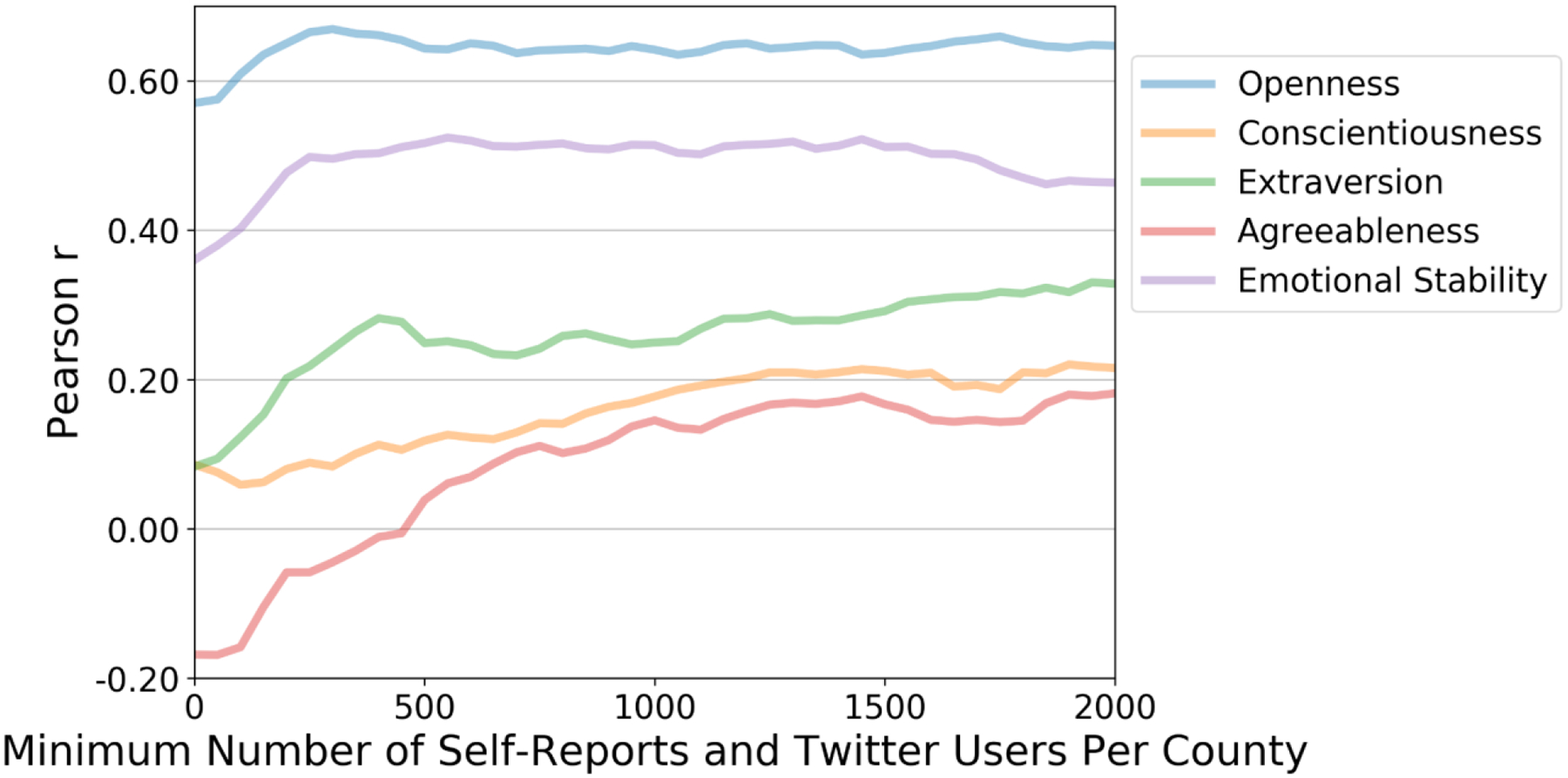
Convergent validity of County-level language-based personality estimates as a function of the minimum number of self-reports and Twitter users per county.

Table 3.

Big 5 personality dimensions and county-level correlates.

	N	Openness	Conscientiousness	Extraversion	Agreeableness	Emotional Stability
% voting Republican (2012 President)	1745	−.24 [−.28, −.20]	.00 [−.04, .05]	.15 [.10, .19]	.05 [.01, .09]	−.07 [−.12, −.03]
% voting Republican (2016 President)	1745	−.41 [−.45, −.37]	−.08 [−.13, −.03]	.24 [.19, .29]	−.02 [−.06, .03]	−.18 [−.23, −.13]
% voting Republican (2020 President)	1719	−.46 [−.51, −.42]	−.12 [−.17, −.07]	.26 [.21, 31]	−.03 [−.07, .02]	−.22 [−.27, −.17]
% management	1749	.40 [.35, .45]	,27 [.20, .33]	−.18 [−.24, −.12]	.13 [.07, .18]	.30 [.24, .36]
% arts and entertainment	1749	.32 [.29, .36]	.20 [.16, .24]	−.02 [−.06, .02]	.08 [.04, .11]	.24 [.20, .28]
% elementary trade	1749	−.43 [−.46, −.39]	−.22 [−.27, −.18]	.15 [.11, .20]	−.08 [−.12, −.04]	−.24 [−.29, −.20]
% bachelors degree	1750	.59 [.55, .64]	.60 [.54, .66]	−.23 [−.29, −.17]	.35 [.30, .40]	.63 [.57, .68]
Patents per 1000 employees	1746	.13 [.09, .17]	,12 [.08, .17]	−.12 [−.16, −.07]	.08 [.04, .12]	.13 [.08, .17]
All-cause mortality	1750	−.25 [−.30, −.20]	−.19 [−.25, −.13]	.05 [−.01, .10]	−.15 [−.20, −.10]	−.32 [−.37, −.26]
% fair or poor health	1688	−.24 [−.29, −.19]	−.31 [−.37, −.26]	.06 [.01, .11]	−.23 [−.28, −.18]	−.32 [−.37, −.26]
Life satisfaction	1573	.17 [.13, .22]	.22 [.17, .27]	−.08 [−.13, −.04]	.19 [.15, .24]	.19 [.14, .23]
% married	1750	−.49 [−.54, −.44]	−.18 [−.24, −.12]	.25 [.19, .31]	−.04 [−.09, .02]	−.20 [−.26, −.14]
% with inadequate social support	1608	−.12 [−.16, −.07]	−.26 [−.31, −.20]	.00 [−.05, .05]	−.19 [−.24, −.15]	−.19 [−.24, −.14]
Violent crime	1665	.17 [.13, .22]	−.02 [−.08, .03]	−.02 [−.07, .03]	−.09 [−.13, −.04]	.05 [−.00, .10]

Note: Reported standardized betas between county-level personality and each outcome. Models include percentage female, median age, log median income, percentage African American, log pop density and a spatially lagged version of the personality dimension. Bolded numbers are significant at p < .05 after a Benjamini-Hochberg FDR correction.

Regional Variation in County-level Personality

To illustrate regional variation, we created county-level choropleths, or map shadings dependent on the traits, shading counties according to z scores. Counties with insufficient Twitter data (i.e., less than 100 users with 30 or more posts) are left blank (white). Figure 2 shows choropleth maps of each of the language-based personality scores per county. All scores are standardized, with purple indicating higher z scores and brown indicating lower z scores.

Figure 2.

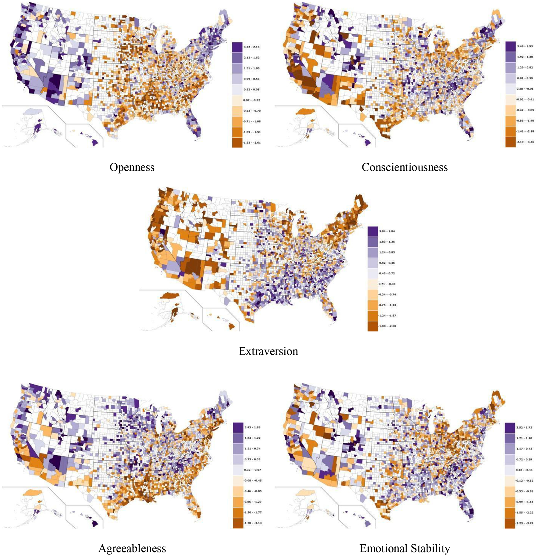
County-level personality dimensions from language-based assessments (white indicates not enough data). Full interactive maps available at map.wwbp.org.

Openness.

Openness (Moran’s I = 0.43, p < 0.001) was generally higher around U.S. coasts, large cities, and throughout the Western states. The most open cities—e.g., Portland (Oregon), San Francisco (California), Seattle (Washington) and Austin (Texas)—also share a reputation for unconventionality, creativity, and innovation. Openness was generally lower in rural areas throughout the Midwest and Southern regions, and the least open counties included suburban areas surrounding Midwestern and mid-Atlantic cities.

Conscientiousness.

Conscientiousness (Moran’s I = 0.30, p < 0.001) had no clear spatial patterns and varied widely within regions and states. The most conscientious counties were found in the Southeast (Alabama, North Carolina, and Florida) with the least conscientious counties in Texas and California.

Extraversion.

County extraversion (Moran’s I = 0.40, p < 0.001) appeared to be greater along a North-South gradient, with introverted the Pacific Northwest and New England being more introverted and the Southeast and southern California being more extraverted. The most extraverted counties included a few areas known for excitement and high social activity, such as Miami and Manhattan; most introverted counties included areas from the Pacific Northwest and East Coast.

Agreeableness.

County agreeableness (Moran’s I = 0.47, p < 0.001) was generally higher across the Western half of the country and the Upland South; agreeableness was particularly low in the Deep South (especially throughout the Stroke Belt) and was low in the heavily populated areas of the East Coast.

Emotional Stability.

Emotional stability (Moran’s I = 0.31, p < 0.001) was generally higher along the country’s southern Sun Belt and in a large cluster of counties in Colorado. Emotional stability was lower throughout the Great Plains and Midwestern regions, particularly in North and South Carolina, Georgia, and Florida.

County-level Correlates

Overview of results.

For each of the five factors we examined their county-level correlation with political, economic, social, health, well-being, and geographic variables. Table 3 shows the correlations between each of the five factors and the 13 PESH variables characterizing each county. Each model contains percentage female, percentage African American, median age, median income, population density, and a spatially lagged personality trait as covariates. Results with and without the spatially lagged variable can be found in Appendix Table A1.

Openness.

More open counties had lower percentages of Republican voters and were more likely to attain at least a bachelor’s level of education. Higher levels of individuals working in the arts is also associated with higher openness. We also see correlations with well-being (positive associations with life satisfaction), heath (lower all-cause mortality and lower percentage poor health), and social support (less inadequate social support).

Conscientiousness.

Increased education, number of patents, and life satisfaction correlated with higher conscientiousness. More conscientious counties were healthier, with significantly lower rates of all-cause mortality and fewer people reporting poor health. More conscientious counties also reported higher rates of social support. We found no significant associations with violent crime rates.

Extraversion.

Extraversion generally had smaller associations with the PESH variables relative to the other factor. Economic variables (education and number of patents) were negatively correlated with extraversion, as was increased Republican voting in the 2012, 2016, and 2020 US elections. Extraverted counties also reported higher poor health and lower life satisfaction. No significant association between extraversion and social support was found.

Agreeableness.

Agreeableness was associated with higher life satisfaction and increased social support. More agreeable counties also had lower all-cause mortality rates and lower violent crime. Republican voting in the 2016 and 2020 elections were not significantly associated with agreeableness, though Republican voting in the 2012 election has a small positive association.

Emotional Stability.

Emotionally stable communities were more likely to complete at least a bachelor’s level of education. We also see associations with increased life satisfaction, higher proportion of professional and managerial occupations, and lower mortality. Violent crime rates have no significant association with emotional stability.

Discussion

Building on past studies of language use and personality, we used county-level language variation to study Big Five dimensions across the U.S. We replicated several findings and extended research on regional personality in terms of spatial resolution by using language-based assessments of personality. Leveraging publicly available social media has therefore reduced the cost, in time and money, of estimating regional personality at finer-grained levels. Because this language-based method relies on behavioral cues (i.e., language behavior), it can be a valuable complement to studies designed around aggregated self-reports.

We found significant personality variation across counties— within U.S. states—suggesting that language-based estimates of personality can provide important nuances. For example, in state-level analyses of openness to experience, Texas falls near the country average (Rentfrow et al., 2008; Rentfrow et al., 2013). However, our county-level analysis reveals rich variation within the state, which contains one of the most open counties in the country (Travis County, Austin, TX; 6th most open) and one of the most conventional (Brazoria, TX; 2nd least open). Additionally, while Palm Beach, FL was the highest in emotional stability, Bradenton, FL was the lowest. Similar patterns were seen in the counties in the large states of California, Arizona, Florida, Pennsylvania, and Ohio, with considerable regional variation across most dimensions.

We also found evidence of broader regional patterns in some dimensions (Figure 2). For example, openness was generally higher in the Western regions, New England, and much of central and coastal Florida. Higher levels of extraversion appeared along a north-south gradient, with the exception of the more sparsely populated Southwest. Agreeableness appears to vary within the stereotypically friendly Southeastern U.S., such that Upland regions are much more agreeable than the Deep South. Our cross-sectional analyses cannot explain how these patterns developed. For instance, historical migration patterns (e.g., more open people traveled and settled farther west), ongoing selective migration (e.g., extraverts are more likely to move from cold northern areas to warmer southern areas), or ecological influence (e.g., heat and humidity cause irritability, increasing disagreeableness in the Deep South), or a combination of these factors might play a role. Future studies that combine our method with longitudinal designs and socio-historical analyses may help tease these influences apart.

The reliability of the county level language estimates (Table 1) dovetails with previous studies that show smaller geographic regions have larger variance explained by the level of aggregation. When compared to the reliabilities reported in Elleman et al. (2020), our results (average ICC1 of 0.047) are closer in size to the zip code level reliabilities than the state level reliabilities, which had reported average values of 0.026 and 0.006, respectively. Similarly sized state level ICC1 values are reported in Elleman et al. (2018). ICC2 results show high group mean reliability and are similar in magnitude to four of the state level samples in Elleman et al. (2018).

While openness and emotional stability showed convergent validity at the county-level (Figure 3), the remaining dimensions were highly dependent on the minimum number of samples (i.e., Twitter users and self-reports) needed per county. After approximately 1000 samples per county, the correlations tended to stabilize, though a slight positive trend exists when increasing above 1000. The low convergent validity when using a small minimum sample size, has a number of possible explanations. First, low population counties could be quantitatively different from high population counties. As one increases the minimum sample threshold, low population counties are dropped from the analysis. For example, when the minimum threshold is set to 2000, less than 400 counties remain. These counties tend to be situated in more rural areas and have distinct socio-demographic profiles when compared to high population urban areas. Additionally, personality estimates at the population level may be unstable when only considering small sample sizes.

At the state-level (Table 2), we see language-based estimates correlate with self-report across three separate datasets, with the exception of agreeableness in Elleman et al. (2018). Across all three samples, openness and emotional stability tend to have the largest correlations, while agreeableness and conscientiousness are the smallest. This roughly matches the county-level results.

Table 2.

Convergent validity of State-level language-based personality estimates.

	Stuetzer et al. (2018)	Rentfrow et al. (2013)	Elleman et al. (2018)
Openness	.77	.69	.55
Conscientiousness	.38	.16	.16
Extraversion	.48	.52	.46
Agreeableness	.13	.58	−.05
Emotional stability	.69	.60	.31

Note: Reported Pearson correlation between state-level language-based personality and self-report. Bolded numbers are significant at p < .05 after a Benjamini-Hochberg FDR correction.

When compared to county-level measures of important life outcomes (Table 3), regional language-based personality estimates replicated many patterns from both individual-level and geographic studies. For example, our results matched individual level studies: more conscientious and emotionally stable counties had lower overall mortality rates (Ozer & Benet-Martinez, 2006; Roberts et al., 2007). More open and conscientious counties had better outcomes on indicators of educational and occupational attainment (graduation rates and income; Ozer & Benet-Martinez, 2006; Roberts et al., 2007). While individual-level correlations, in general, are not expected to replicate at the group level, consistency across individual- and county-level correlates aligns with predictions from the dynamic-process model elaborated by Rentfrow et al. (2008). According to this model, distributions of individual-level traits within a region gradually become linked to regional measures of conceptually related psychological and behavioral outcomes. This can occur through bottom-up paths (e.g., more open individuals are more likely to vote for liberal candidates and, in aggregate, groups of more open people will have a higher proportion of similar votes) or through top-down paths (e.g., areas that consistently elect more liberal candidates tend to attract more open individuals).

The county-level associations between conscientiousness and PESH indicators largely aligned with the patterns found in individual-level research. More conscientious counties had higher educational attainment, lower mortality rates, better social support, and greater life satisfaction. Our results are consistent with individual-leveling findings (e.g., Kern & Friedman, 2008; Ozer & Benet-Martinez, 2000; Roberts et al., 2007), unlike several analyses that found the opposite patterns when using regional averages of conscientiousness based on self-reports (Rentfrow et al. 2008, 2013; Wood & Rogers, 2011; Elleman et al, 2018, 2020), potentially due, in part, to reference group effects.

Why would the language-based county-level estimates not also be biased by these effects? The language-based model was fit across a population of individuals spanning heterogeneous regions, without geographic information about the individuals producing the language, though we note that linguistic features carry their own bias (including geographic biases). If an individual’s self-reported conscientiousness is biased by the RGE, it would add statistical noise to the model, but this would not systematically bias the predictions of the language-based model. To reproduce the RGE with the language-based estimates, geographic information could be included in the model (for example, by adding geographic indicators, or by training separate models for each geographic region). However, because our model is built over a sample of geographically diverse individuals, the predictions are based on generalized, regionally independent relationships between language features and self-reported personality.

Finally, there is evidence that language-based personality estimates do not suffer as extensively from RGE errors. Youyou et al. (2017) showed that romantic partners exhibited similar personality when measured through behavior-based methods (i.e., language and a variety of other behavior on social media), as opposed to self and peer-reported questionnaires. The language-based personality models were trained to account for shared language between romantic partners by building models on disjoint sets of words, thus controlling for any RGE errors. Since similar methods were used to train the personality model applied in the current study, the language-based estimates should not contain the same extent of self report biases.

Limitations

This work is part of a developing line of research that attempts to assess a traditionally individual characteristic, personality, at the regional level. Regional personality provides a framework for studying the community psychological characteristics affecting well-being of communities. Our approach and findings suggest that these variations can be measured efficiently and at scale using computational linguistic analysis methods.

While we have offered several directions forward for this line of study, our approach also has several important limitations. First, while social media can provide massive quantities of behavioral data, its users are not fully representative of the population. The current study relied on data from 2009–2015. As of 2019, 22% of online adults use Twitter, with the majority of users between 18 and 29 years of age (Perrin & Anderson, 2019). Our regional estimates are therefore influenced by the personalities of Twitter users from each region, not necessarily the broader population within those regions. Further, groups of individuals may be more homogenous, heterogeneous, or even highly polarized in their distribution of personality traits from county to county. We attempted to counter this by comparing these estimates to representative outcomes, and we did indeed find several correlations that aligned with our predictions, suggesting that this subpopulation contains useful information about regional variation in the population at large. Previous studies have validated that non-representative social media-based regional features can still predict representative health or survey data (Eichstaedt et al., 2015; Kern et al., 2016; Schwartz et al., 2013b).

Future studies might augment public random feed data with more extensive data collection from individuals within a county. However, research on social media users suggests that representativeness is improving as it continues to be adopted by the general population (as of 2019 almost 70% of U.S. adults use Facebook; Perrin & Anderson, 2019). Social media-based methods should become more relevant and reliable as these technologies become further integrated into the everyday life of the population.

Second, language-based assessments suffer from semantic drifts as language changes over time. Jaidka et al. (2018) showed that models trained on social media language to predict age and gender experienced diminished predictive accuracy as the time difference between the training and testing data grew. The study also showed that certain groups experience drift faster than others: language changes more year to year in younger users (late teen and early twenties) than older users (mid-thirties). Thus, we might expect a range of accuracies when applying language models trained on a specific time period to data from large, diverse populations at another time period.

Finally, the language model developed by Park et al., (2015) has limitations, including relatively lower discriminant validity for the language-based estimates than self-report based scores. As noted by Park et al., one explanation for lower lower discrimination is that traits correlate with shared language (e.g., both conscientiousness and agreeableness positively correlate with “great” and “wonderful”). This shared language could also drive similar correlations at the county-level. Additionally, Park et al. found correlations with self-report external criteria higher for self-report based measures than with language estimates, while language-based assessments had the same or greater correlations with external criteria that was not based on self-report. When compared to Ebert et al. (2019), we find correlations with external criteria have similar effect sizes with both language-based and self-report based measures.

Conclusion

Geographic regions in the U.S. have long been associated with stereotypes about their distinguishing characteristics – or the “personality” of places. This study empirically explores these geographical personality assumptions using aggregate, language-based estimates of personality in counties across the U.S. We found that personality does indeed systematically vary across geography and that language-based estimates are able to track this variation. In addition, we found that other factors (such as political views, economics, social factors, health outcomes, and well-being) correlate with personality dimensions on the county level similarly to how they have been found to correlate in previous studies of survey-based geographic personality. Furthermore, these correlations are shown to be robust to spatial confounds. While this study explored personality and PESH outcomes on the county level using natural language from a large social media database, this method could be used to explore other factors across geographic regions. The current findings, and this method more generally, may have particular relevance to future country-wide policy, health, and well-being research.

Appendix

Table A1.

Big 5 personality traits and county-level correlates with and without controlling for spatial autocorrelation.

	Openness				Conscientiousness				Extraversion				Agreeableness				Emotional Stability
	OLS β	OLS auto.	Spat. β	Spat. auto.	OLS β	OLS auto.	Spat. β	Spat. auto.	OLS β	OLS auto.	Spat. β	Spat. auto.	OLS β	OLS auto.	Spat. β	Spat. auto.	OLS β	OLS auto.	Spat. β	Spat. auto.
% voting Republican (2012 President)	−.34	.39	−.24	.05	.05	.29	.00	−.13	.30	.22	.15	−.10	.03	.32	.05	−.08	−.04	.25	−.07	−.08
% voting Republican (2016 President)	−.51	.36	−.41	.10	−.05	.30	−.08	−.12	.40	.18	.24	−.09	−.05	.32	−.02	−.08	−.17	.26	−.18	−.06
% voting Republican (2020 President)	−.56	.37	−.46	.12	−.10	.30	−.12	−.12	.43	.18	.26	−.09	−.07	.32	−.03	−.07	−.22	.27	−.22	−.06
% management	.51	.33	.40	.03	.35	.29	.27	−.10	−.23	.27	−.18	−.12	.15	.32	.13	−.08	.38	.23	.30	−.05
% arts and entertainment	.38	.32	.32	−.01	.20	.31	.20	−.12	−.06	.27	−.02	−.12	.09	.33	.08	−.07	.26	.24	.24	−.07
% elementary trade	−.51	.34	−.43	.07	−.24	.32	−.22	−.10	.24	.24	.15	−.11	−.05	.33	−.08	−.07	−.26	.26	−.24	−.05
% bachelors degree	.66	.38	.59	.06	.68	.30	.60	−.05	−.34	.23	−.23	−.12	.42	.32	.35	−.05	.67	.25	.63	−.02
patents per 1000 employees	.16	.39	.13	.00	.10	.30	.12	−.13	−.17	.27	−.12	−.12	.10	.32	.08	−.07	.12	.25	.13	−.08
All-cause mortality	−.33	.38	−.25	.01	−.18	.31	−.19	−.12	.15	.26	.05	−.12	−.20	.33	−.15	−.06	−.35	.25	−.32	−.06
% fair or poor health	−.24	.44	−.24	.02	−.35	.30	−.31	−.10	.11	.27	.06	−.12	−.31	.31	−.23	−.05	−.31	.26	−.32	−.07
Life satisfaction	.15	.41	.17	−.02	.29	.27	.22	−.12	−.04	.28	−.08	−.13	.22	.30	.19	−.08	.24	.22	.19	−.07
% married	−.61	.35	−.49	.07	−.12	.31	−.18	−.12	.41	.22	.25	−.10	.02	.31	−.04	−.08	−.17	.26	−.20	−.07
% with adequate social support	−.05	.42	−.12	−.01	−.32	.26	−.26	−.11	−.02	.28	.00	−.12	−.28	.26	−.19	−.06	−.20	.23	−.19	−.07
violent crime	.22	.36	.17	−.01	−.05	.29	−.02	−.13	−.02	.28	−.02	−.12	−.11	.31	−.09	−.08	.07	.24	.05	−.07

Note: Reported standardized betas between county-level personality and each outcome as well as Moran’s I computed on the models’ residuals. Each model includes percentage female, median age, log median income, percentage African American, and log pop density. Bolded Moran’s I values are significant at p < .05

References

- Allik J, & McCrae RR (2004). Toward a geography of personality traits: Patterns of profiles across 36 cultures. Journal of Cross Cultural Psychology, 35, 13–28. [Google Scholar]
- Atkins DC, Rubin TN, Steyvers M, Doeden MA, Baucom BR, & Christensen A (2012). Topic models: A novel method for modeling couple and family text data. Journal of Family Psychology, 26, 816–827. 10.1037/a0029607 [DOI] [PMC free article] [PubMed] [Google Scholar]
- Arbia G (2014). A primer for spatial econometrics with applications in R. Palgrave Macmillan. [Google Scholar]
- Back MD, Stopfer JM, Vazire S, Gaddis S, Schmukle SC, Egloff B, & Gosling SD (2010). Facebook profiles reflect actual personality, not self-idealization. Psychological Science, 21, 372–374. 10.1177/0956797609360756 [DOI] [PubMed] [Google Scholar]
- Benjamini Y, & Hochberg Y (1995). Controlling the false discovery rate: a practical and powerful approach to multiple testing. Journal of the Royal statistical society: series B (Methodological), 57(1), 289–300. [Google Scholar]
- Blei DM, Ng AY, & Jordan MI (2003). Latent dirichlet allocation. Journal of Machine Learning Research, 3, 993–1022. [Google Scholar]
- Bleidorn W, Schönbrodt F, Gebauer JE, Rentfrow PJ, Potter J, & Gosling SD (2016). To live among like-minded others: Exploring the links between personality-city fit and self-esteem. Psychological Science, 27, 419–427. [DOI] [PubMed] [Google Scholar]
- Bliese PD (2000). Within-group agreement, non-independence, and reliability: Implications for data aggregation and analysis. [Google Scholar]
- Condon DM Roney E, & Revelle W (2018). Selected personality data from the SAPA-Project: 22Dec2015 to 07Feb2107. Harvard Dataverse. [Google Scholar]
- Costa PT Jr., & McCrae RR (1992). Revised NEO Personality Inventory (Neo-PI-R) and NEO Five-Factor Inventory (NEO-FFI): Professional manual. Odessa, FL: Psychological Assessment Resources. [Google Scholar]
- Culotta A (2014). Estimating county health statistics with twitter. In Proceedings of the SIGCHI Conference on Human Factors in Computing Systems (pp. 1335–1344). [Google Scholar]
- Curtis B, Giorgi S, Buffone AE, Ungar LH, Ashford RD, Hemmons J, … & Schwartz HA (2018). Can Twitter be used to predict county excessive alcohol consumption rates?. PloS one, 13(4), e0194290. [DOI] [PMC free article] [PubMed] [Google Scholar]
- DeNeve KM, & Cooper H (1998). The happy personality: A meta-analysis of 137 personality traits and subjective well-being. Psychological Bulletin, 124, 197–229. [DOI] [PubMed] [Google Scholar]
- Ebert T, Gebauer JE, Brenner T, Bleidorn W, Gosling SD, Potter J, & Rentfrow PJ (2019). Are regional differences in personality and their correlates robust? Applying spatial analysis techniques to examine regional variation in personality across the U.S. and Germany. (Working Papers on Innovation and Space No. 2019.05). Philipps University Marburg. [DOI] [PubMed] [Google Scholar]
- Eichstaedt JC, Schwartz HA, Kern ML, Park G, Labarthe DR, Merchant RM, Jha S, Agrawal M, Dziurzynski LA, Sap M, Weeg C, Larson EE, Ungar LH, & Seligman ME (2015). Psychological Language on Twitter Predicts County-Level Heart Disease Mortality. Psychological Science, 26, 159–169. [DOI] [PMC free article] [PubMed] [Google Scholar]
- Elleman LG, Condon DM, Russin SE, & Revelle W (2018). The personality of U.S. states: Stability from 1999 to 2015. Journal of Research in Personality, 72, 64–72. [DOI] [PMC free article] [PubMed] [Google Scholar]
- Elleman L, Condon DM, Holtzman NS, Allen VR, & Revelle W (2020). Smaller is better: Associations between personality and demographics are improved by examining narrower traits and regions.
- Entringer TM, Gebauer JE, Eck J, Bleidorn W, Rentfrow PJ, Potter J, & Gosling SD (2021). Big Five facets and religiosity: Three large-scale, cross-cultural, theory-driven, and process-attentive tests. Journal of Personality and Social Psychology, 120(6), 1662. [DOI] [PubMed] [Google Scholar]
- Gebauer JE, Sedikides C, Schönbrodt FD, Bleidorn W, Rentfrow PJ, Potter J, & Gosling SD (2017). The religiosity as social value hypothesis: A multi-method replication and extension across 65 countries and three levels of spatial aggregation. Journal of Personality and Social Psychology, 113(3), e18. [DOI] [PubMed] [Google Scholar]
- Getis A, & Aldstadt J (2004). Constructing the spatial weights matrix using a local statistic. Geographical analysis, 36(2), 90–104. [Google Scholar]
- Giorgi S, Preoţiuc-Pietro D, Buffone A, Rieman D, Ungar L, & Schwartz HA (2018, November). The remarkable benefit of user-level aggregation for lexical-based population-level predictions. Paper presented at the 2018 Conference on Empirical Methods in Natural Language Processing, Brussels, Belgium. [Google Scholar]
- Giorgi Salvatore, Lynn Veronica, Matz Sandra, Ungar Lyle, and Schwartz H. Andrew. “Correcting Sociodemographic Selection Biases for Accurate Population Prediction from Social Media.” arXiv preprint arXiv:1911.03855 (2019). [PMC free article] [PubMed] [Google Scholar]
- Greene WH (2000). Econometric analysis. Upper Saddle River, N.J: Prentice Hall. [Google Scholar]
- Gosling S, Vazire S, Srivastava S, John O (2004). Should we trust web-based studies? A comparative analysis of six preconceptions about internet questionnaires. American Psychologist, 59, 93–104. [DOI] [PubMed] [Google Scholar]
- Heine SJ, Buchtel EE, & Norenzayan A (2008). What do cross-national comparisons of personality traits tell us? The case of conscientiousness. Psychological Science, 19(4), 309–313. [DOI] [PubMed] [Google Scholar]
- Heine SJ, Lehman DR, Peng K, & Greenholtz J (2002). What’s wrong with cross-cultural comparisons of subjective likert scales?: The reference-group effect. Journal of Personality and Social Psychology, 82(6), 903–918. [PubMed] [Google Scholar]
- Jaidka K, Chhaya N, & Ungar L (2018). Diachronic degradation of language models: Insights from social media. In Proceedings of the 56th Annual Meeting of the Association for Computational Linguistics (Volume 2: Short Papers) (pp. 195–200). [Google Scholar]
- Jaidka K, Giorgi S, Schwartz HA, Kern ML, Ungar LH, & Eichstaedt JC (2020). Estimating geographic subjective well-being from Twitter: A comparison of dictionary and data-driven language methods. Proceedings of the National Academy of Sciences, 117(19), 10165–10171. [DOI] [PMC free article] [PubMed] [Google Scholar]
- John OP, & Srivastava S (1999). The Big Five trait taxonomy: History, measurement, and theoretical perspectives. In Pervin LA, & John OP (Eds.), Handbook of personality: Theory and research (pp. 102–138). New York: Guilford Press. [Google Scholar]
- Jokela M, Bleidorn W, Lamb ME, Gosling SD, & Rentfrow PJ (2015). Geographically varying associations between personality and life satisfaction in the London metropolitan area. Proceedings of the National Academy of Sciences, 112, 725–730. [DOI] [PMC free article] [PubMed] [Google Scholar]
- Jost JT, Glaser J, Kruglanski AW, & Sulloway FJ (2003). Political conservatism as motivated social cognition. Psychological Bulletin, 129, 339–375. [DOI] [PubMed] [Google Scholar]
- Kern ML, & Friedman HS (2008). Do conscientious individuals live longer? A quantitative review. Health Psychology, 27, 505–512. [DOI] [PubMed] [Google Scholar]
- Kern ML, Friedman HS, Martin LR, Reynolds CA, & Luong G (2009). Conscientiousness, career success, and longevity: A lifespan analysis. Annals of Behavioral Medicine, 37, 154–163. [DOI] [PMC free article] [PubMed] [Google Scholar]
- Kern ML, Eichstaedt JC, Schwartz HA, Dziurzynski L, Ungar LH, Stillwell DJ, … & Seligman MEP (2014). The online social self: An open vocabulary approach to personality. Assessment, 21, 158–169. 10.1177/1073191113514104 [DOI] [PubMed] [Google Scholar]
- Kern ML, Park G, Eichstaedt JC, Schwartz HA, Sap M, Smith LK, & Ungar LH (2016). Gaining insights from social media language: Methodologies and challenges. Psychological methods, 21(4), 507. [DOI] [PubMed] [Google Scholar]
- Krug SE, & Kulhavy RW (1973). Personality differences across regions of the United States. The Journal of Social Psychology, 91, 73–79. [DOI] [PubMed] [Google Scholar]
- Lawless NM & Lucas RE (2011). Predictors of regional well-being: A county-level analysis. Social Indicators Research, 101, 341–357. [Google Scholar]
- Leip D (2016). Dave Leip U.S. Presidential General County Election Results, 10.7910/DVN/SUCQ52, Harvard Dataverse, V5, UNF:6:VyZqxCIVvvY/CYunVWVc0g== [fileUNF] [DOI]
- Leip D (2020). Dave Leip’s Atlas of U.S. Presidential Elections. http://uselectionatlas.org.
- Levine RV, & Norenzayan A (1999). The pace of life in 31 counties. Journal of Cross-Cultural Psychology, 30, 178–205. [Google Scholar]
- Lui M, & Baldwin T (2012). langid. py: An off-the-shelf language identification tool. In Proceedings of the ACL 2012 system demonstrations (pp. 25–30). Association for Computational Linguistics. [Google Scholar]
- Martinsson PG, Rokhlin V, & Tygert M (2011). A randomized algorithm for the decomposition of matrices. Applied and Computational Harmonic Analysis, 30(1), 47–68. [Google Scholar]
- McCrae RR (1996). Social consequences of experiential openness. Psychological Bulletin, 120, 323–337. [DOI] [PubMed] [Google Scholar]
- McCrae RR, Terracciano A, & 79 Members of the Personality Profiles of Cultures Project. (2005). Personality profiles of cultures: Aggregate personality traits. Journal of Personality and Social Psychology, 89, 407–425. [DOI] [PubMed] [Google Scholar]
- Moran PA (1950). Notes on continuous stochastic phenomena. Biometrika, 37, 17–23. [PubMed] [Google Scholar]
- Naaman M, Boase J, & Lai CH (2010). Is it really about me?: Message content in social awareness streams. In Proceedings of the 2010 ACM conference on Computer Supported Cooperative Work (pp. 189–192). Retrieved at: http://luci.ics.uci.edu/predeployment/websiteContent/weAreLuci/biographies/faculty/djp3/LocalCopy/p189-naaman.pdf [Google Scholar]
- Obschonka M, Lee N, Rodríguez-Pose A, Eichstaedt JC, & Ebert T (2019). Big data methods, social media, and the psychology of entrepreneurial regions: Capturing cross-county personality traits and their impact on entrepreneurship in the USA. Small Business Economics, 1–22. [Google Scholar]
- Obschonka M, Schmitt-Rodermund E, Silbereisen RK, Gosling SD, & Potter J (2013). The regional distribution and correlates of an entrepreneurship-prone personality profile in the United States, Germany, and the United Kingdom: A socioecological perspective. Journal of Personality and Social Psychology, 105, 104–122. [DOI] [PubMed] [Google Scholar]
- Obschonka M, Stuetzer M, Audretsch DB, Rentfrow PJ, Potter J, & Gosling SD (2016). Macro-psychological factors predict regional economic resilience during a major economic crisis. Social Psychology and Personality Science, 7, 95–104. [Google Scholar]
- Ozer DJ, & Benet-Martinez V (2006). Personality and the prediction of consequential outcomes. Annual Review of Psychology, 57, 401–421. [DOI] [PubMed] [Google Scholar]
- Park N, Peterson C, & Seligman ME (2006). Character strengths in fifty-four nations and the fifty US states. The Journal of Positive Psychology, 1, 118–129. [Google Scholar]
- Park G, Schwartz HA, Eichstaedt JC, Kern ML, Kosinski M, Stillwell DJ, … & Seligman ME (2015). Automatic personality assessment through social media language. Journal of Personality and Social Psychology, 108(6), 934. [DOI] [PubMed] [Google Scholar]
- Pennebaker JW, & King LA (1999). Linguistic styles: Language use as an individual difference. Journal of Personality and Social Psychology, 77, 1296–1312. 10.1037/0022-3514.77.6.1296 [DOI] [PubMed] [Google Scholar]
- Pennebaker JW, Mehl MR, & Niederhoffer KG (2003). Psychological aspects of natural language use: Our words, our selves. Annual Review of Psychology, 54, 547–577. 10.1146/annurev.psych.54.101601.145041 [DOI] [PubMed] [Google Scholar]
- Perrin A & Anderson M (2019). Share of U.S. adults using social media, including Facebook, is mostly unchanged since 2018. Pew Research Center. Available at: https://www.pewresearch.org/fact-tank/2019/04/10/share-of-u-s-adults-using-social-media-including-facebook-is-mostly-unchanged-since-2018/
- Pressman SD, & Cohen S (2005). Does positive affect influence health? Psychological Bulletin, 131, 925–971. [DOI] [PubMed] [Google Scholar]
- Preotiuc-Pietro D, Samangooei S, Cohn T, Gibbins N, & Niranjan M (2012). Trendminer: An architecture for real time analysis of social media text. [Google Scholar]
- Remington PL, Catlin BB, & Gennuso KP (2015). The county health rankings: rationale and methods. Population health metrics, 13(1), 11. [DOI] [PMC free article] [PubMed] [Google Scholar]
- Rentfrow PJ, Gosling SD, & Potter J (2008). A theory of the emergence, persistence, and expression of geographic variation in psychological characteristics. Perspectives on Psychological Science, 3, 339–369. [DOI] [PubMed] [Google Scholar]
- Rentfrow PJ, Jost JT, Gosling SD, & Potter J (2009). Statewide differences in personality predict voting patterns in 1996–2004 US presidential elections. Social and psychological bases of ideology and system justification, 1, 314–349. [Google Scholar]
- Rentfrow PJ (2010). Statewide differences in personality: Toward a psychological geography of the United States. American Psychologist, 65, 548–558. [DOI] [PubMed] [Google Scholar]
- Rentfrow PJ, Gosling SD, Jokela M, Stillwell DJ, Kosinski M, & Potter J (2013). Divided we stand: Three psychological regions of the United States and their political, economic, social, and health correlates. Journal of Personality and Social Psychology, 105, 996–1012. [DOI] [PubMed] [Google Scholar]
- Rentfrow PJ, Jokela M, & Lamb ME (2015). Regional personality differences in Great Britain. PLOS One, 10, e0122245. [DOI] [PMC free article] [PubMed] [Google Scholar]
- Rentfrow PJ, & Jokela M (2016). Geographical psychology: The spatial organization of psychological phenomena. Current Directions in Psychological Science, 25, 393–398. [Google Scholar]
- Rentfrow PJ, Mellander C, & Florida R (2009). Happy states of America: A state-level analysis of psychological, economic, and social well-being. Journal of Research in Personality, 43, 1073–1082. [Google Scholar]
- Rieman D, Jaidka K, Schwartz HA, & Ungar L (2017). Domain adaptation from user-level facebook models to county-level twitter predictions. In Proceedings of the Eighth International Joint Conference on Natural Language Processing (Volume 1: Long Papers) (Vol. 1, pp. 764–773). [Google Scholar]
- Roberts BW, Lejuez C, Krueger RF, Richards JM, & Hill PL (2014). What is conscientiousness and how can it be assessed? Developmental Psychology, 50, 1315–1330. doi: 10.1037/a0031109 [DOI] [PubMed] [Google Scholar]
- Roberts BW, Kuncel NR, Shiner R, Caspi A, & Goldberg LR (2007). The power of personality: The comparative validity of personality traits, socioeconomic status, and cognitive ability for predicting important life outcomes. Perspectives on Psychological Science, 2, 313–345. [DOI] [PMC free article] [PubMed] [Google Scholar]
- Rogers KH, & Wood D (2010). Accuracy of United States regional personality stereotypes. Journal of Research in Personality, 44, 704–713. [Google Scholar]
- Schwartz HA, Eichstaedt JC, Kern ML, Dziurzynski L, Agrawal M, Park G, … & Ungar LH (2013a). Characterizing geographic variation in well-being using tweets. Paper presented in the Seventh International AAAI Conference on Weblogs and Social Media, Boston, MA. [Google Scholar]
- Schwartz HA, Eichstaedt JC, Kern ML, Dziurzynski L, Ramones SM, Agrawal M, …, & Ungar LH (2013b). Personality, gender, and age in the language of social media: The open vocabulary approach. PLOS ONE, 8, e73791. 10.1371/journal.pone.0073791 [DOI] [PMC free article] [PubMed] [Google Scholar]
- Stuetzer M, Audretsch DB, Obschonka M, Gosling SD, Rentfrow PJ, & Potter J (2018) Entrepreneurship culture, knowledge spillovers and the growth of regions, Regional Studies, 52, 608–618. [Google Scholar]
- Tausczik Y, & Pennebaker JW (2010). The psychological meaning of words: LIWC and computerized text analysis methods. Journal of Language and Social Psychology, 29, 24–54. 10.1177/0261927X09351676 [DOI] [Google Scholar]
- Tobler WR (1970). A computer movie simulating urban growth in the Detroit region. Economic Geography, 46, 234–240. [Google Scholar]
- United States Patent and Trademark Office (2020). U.S. State Patenting Breakout by Regional Component. Retrieved August, 2020 from https://www.uspto.gov/web/offices/ac/ido/oeip/taf/countyall/usa_county_gd.htm.
- Vazire S, & Carlson EN (2011). Others sometimes know us better than we know ourselves. Current Directions in Psychological Science, 20, 104–108. 10.1177/0963721411402478 [DOI] [Google Scholar]
- Von Elm E, Altman DG, Egger M, Pocock SJ, Gøtzsche PC, & Vandenbroucke JP (2007). The Strengthening the Reporting of Observational Studies in Epidemiology (STROBE) statement: guidelines for reporting observational studies. Bulletin of the World Health Organization, 85, 867–872. [DOI] [PMC free article] [PubMed] [Google Scholar]
- Ward MD, & Gleditsch KS (2018). Spatial regression models (Vol. 155). Sage Publications. [Google Scholar]
- Wei W, Lu JG, Galinsky AD, Wu H, Gosling SD, Rentfrow PJ, … Wang L (2017). Regional ambient temperature is associated with human personality. Nature Human Behavior, 1, 890–895. [DOI] [PubMed] [Google Scholar]
- Wood D, & Rogers KH (2011). Regional differences in personality exist, but how do we get to them? The case of conscientiousness. American Psychologist, 66, 917–918. [DOI] [PubMed] [Google Scholar]
- Yarkoni T (2010). Personality in 100,000 words: A large-scale analysis of personality and word use among bloggers. Journal of Research in Personality, 44, 363–373. 10.1016/j.jrp.2010.04.001 [DOI] [PMC free article] [PubMed] [Google Scholar]
- Youyou W, Stillwell D, Schwartz HA, & Kosinski M (2017). Birds of a feather do flock together: Behavior-based personality-assessment method reveals personality similarity among couples and friends. Psychological science, 28(3), 276–284. [DOI] [PubMed] [Google Scholar]