Coupled generation

Abstract

Instance generation creates representative examples to interpret a learning model, as in regression and classification. For example, representative sentences of a topic of interest describe the topic specifically for sentence categorization. In such a situation, a large number of unlabeled observations may be available in addition to labeled data, for example, many unclassified text corpora (unlabeled instances) are available with only a few classified sentences (labeled instances). In this article, we introduce a novel generative method, called a coupled generator, producing instances given a specific learning outcome, based on indirect and direct generators. The indirect generator uses the inverse principle to yield the corresponding inverse probability, enabling to generate instances by leveraging an unlabeled data. The direct generator learns the distribution of an instance given its learning outcome. Then, the coupled generator seeks the best one from the indirect and direct generators, which is designed to enjoy the benefits of both and deliver higher generation accuracy. For sentence generation given a topic, we develop an embedding-based regression/classification in conjuncture with an unconditional recurrent neural network for the indirect generator, whereas a conditional recurrent neural network is natural for the corresponding direct generator. Moreover, we derive finite-sample generation error bounds for the indirect and direct generators to reveal the generative aspects of both methods thus explaining the benefits of the coupled generator. Finally, we apply the proposed methods to a real benchmark of abstract classification and demonstrate that the coupled generator composes reasonably good sentences from a dictionary to describe a specific topic of interest.

1. Introduction

Generating an essay or a text for given structured information is an important Artificial Intelligence (AI) problem, which automatically imitates a certain style of writing. Whereas solving this AI problem is rather challenging, we tackle its simpler version in this article, which we call instance (example) generation, that is, generation of representative instances given a specific outcome to describe and interpret the corresponding learning model, for instance, classification and regression.

The use of black-box predictive models such as deep neural networks has delivered a high empirical learning accuracy in many real-life applications [14, 15]. Yet, it is difficult to make a sense of such a learning model. From the generative perspective, instance generation can describe the relationship between an instance and an outcome retrospectively. Its applications include a topic description of sentence categorization, abstractive text summarization [12], and image captioning [25], where generated sentences render descriptive examples of topics, texts, and images. In such a situation, sentence generation allows us to compose a novel essay and image captioning when the structured information is supplied. For example, the UCI abstract categorization benchmark¹ consists of sentences from abstracts of articles, which are labeled with one of five topic categories. The goal here is learning a sentence generation mechanism to compose a novel abstract given a specific topic, in which the generation performance is measured by the cross-entropy error based on a test sample.

In the literature, instance generation, despite its vast important applications in AI, remains largely unexplored, although some approaches have been suggested for sentence generation. For example, a computational linguistics approach represents words/phrases as trees to model linguistic dependencies [20], a learning approach uses a large text corpus to learn a sentence’s structure without any access to linguistic annotation [5]. In [26], a sentence generating model is proposed to produce a document by sampling the latent topic of a sentence and then words of the sentence using a recurrent neural network (RNN). In [37, 17], image captioning links the image content to a language model through an interplay between a convolution neural network (CNN) and an RNN. Yet, there is a paucity of works on instance generation given structured information, and incorporating both labeled and unlabeled data.

One of the primary characteristics of topic-instance data is that the amount of unlabeled data may be significantly larger than that of labeled data. For example, in sentence generation, uncategorized sentences are about ten times more than categorized ones. This is in a parallel situation of semisupervised learning with a different focus on leveraging unlabeled data to enhance the predictive accuracy of supervised learning [42, 18], which is in contrast to our generation objective given a learning outcome.

Our main contribution lies in the development of a new semisupervised generation framework for producing instances given an outcome. On this ground, we propose three generative methods–indirect, direct, and coupled generators. The indirect generator uses the principle of inverse learning to estimate the conditional probability distribution of an outcome given an instance, enabling to leverage unlabeled data, if available. On the other hand, the direct generator estimates the corresponding conditional probability of an instance given an outcome in a supervised manner. Then, the coupled generator is designed to enjoy the benefits of both generations. The proposed generators are illustrated in sentence generation, where we generate a sentence through sequential next-word-prediction. Specifically, we develop regularized embedding-based regression/classification in conjuncture with an unconditional RNN for the indirect generator, whereas we use a conditional RNN for the direct generator.

To shed light on the generative performance of the three generators, we derive finite-sample generation error bounds for each method. Interestingly, the generation error of the indirect generator is governed by the complexity of the parameter space of the conditional densities of an outcome given an instance and that of marginal densities. Similarly, that of the direct generator is determined by the conditional densities of an instance given an outcome. As a result, the indirect and direct generators have their own advantages with respect to generation with the unlabeled data is large, and importantly the coupled generator enjoys the benefits of both in terms of generation accuracy. This, together with a real benchmark of sentence categorization, demonstrates the utility of the coupled generation for composing reasonably good sentences to describe a specific topic. Numerically, the proposed method outperforms a separate RNN method and the indirect generator can leverage additional unlabeled data for further enhancing the performance.

This paper is organized as follows. Section 2 introduces the framework of coupled generation based on indirect and direct generations. Section 3 develops a theory of the generation performance of the proposed methods. Section 4 is devoted to the development of a novel sentence generative method given a topic of interest through sequential next-word prediction. Section 5 investigates the operating characteristics of the coupled generator and compares it with the direct and indirect generators as well as one competitor. The Appendix contains technical proofs.

2. Methods

Consider a generative model in which the goal is to generate an instance X given an outcome Y, where X and Y represent instance and response variables, which can be numerical or unstructured such as texts and documents that cannot be expressed in a predefined manner. In this article, we focus on instance generation under a generative model, based on the conditional distribution p_X|Y of X given an outcome of Y. As an example, in sentence generation [26], instance generation produces representative examples of X given a specific topic of Y, where X and Y represent a sentence and its associated topic.

For instance generation, a labeled training sample ${\left(x^i,y^i\right)}_{i=1}^n$ is available as well as an instance-only sample ${\left(x^j\right)}_{j=1}^{\tilde{n}}$, whose sample size $\tilde{n}$ may greatly exceed or smaller than the sample size n. In our context, we leverage the unlabeled sample to enhance the generative accuracy of instance generation.

Indirect generator.

An indirect generator produces instances using an estimate of p_X|Y through the inverse relation (1): an estimate of p_Y|X based on ${\left(x^i,y^i\right)}_{i=1}^n$ in (2) and the marginal density p_X based on combined data ${\left(x^i\right)}_{i=1}^n$ and ${\left(x^j\right)}_{j=1}^{\tilde{n}}$ in (3). That is,

$$\text{Indirect}:{\widehat{p}}_{X|Y}^b(x\mid y)=\frac{{\widehat{p}}_{Y|X}(y\mid x){\widehat{p}}_X(x)}{{\int }_{x\in \mathcal{X}}{\widehat{p}}_{Y\mid X}(y\mid x){\widehat{p}}_X(x)dx},$$ (1)

$${\widehat{p}}_{Y\mid X}=\underset{p_{Y|X}\in {\mathcal{F}}_b}{\text{argmin}}-n^{-1}\sum _{i=1}^n\text{log}\left(p_{Y\mid X}\left(y^i\mid x^i\right)\right)+{\lambda }_b{J}_b\left(p_{Y\mid X}\right),$$ (2)

$${\widehat{p}}_X=\underset{p_X\in {\mathcal{F}}_m}{\text{argmin}}-{(n+\tilde{n})}^{-1}\left(\sum _{i=1}^n\text{log}\left(p_X\left(x^i\right)\right)+\sum _{j=1}^{\tilde{n}}\text{log}\left(p_X\left(x^j\right)\right)\right)+{\lambda }_m{J}_m\left(p_X\right),$$ (3)

where ${\widehat{p}}_{Y\mid X}$ and ${\widehat{p}}_X$ in (1) are regularized maximum likelihood estimates of p_Y|X and p_X, J_b and J_m are regularizers, for example, L₁- or L₂-regularization in a neural network model, λ_b ≥ 0 and λ_m ≥ 0 are tuning parameters controlling the weights of regularization, and ${\mathcal{F}}_b$ in (2) and ${\mathcal{F}}_m$ in (3) are parameter spaces of p_Y|X and p_X, respectively. Note that ${\int }_{x\in \mathcal{X}}{\widehat{p}}_{X\mid Y}(x\mid y){\widehat{p}}_X(x)dx$ in (1) normalizes ${\widehat{p}}_{X\mid Y}^b$ to become a probability density, although normalization is unnecessary when only some aspects of the distribution such as the modes or percentiles are of concern, as opposed to the distribution itself. Importantly, the indirect generator leverages instance-only (unlabeled) data ${\left(x^j\right)}_{j=1}^{\tilde{n}}$, but any potential bias in estimation of p_X based on ${\left(x^j\right)}_{j=1}^{\tilde{n}}$ could translate into that of p_Y|X.

Direct generator.

A direct generator uses p_X|Y to generate instances, estimated by minimizing the negative regularized conditional likelihood of X given Y based on ${\left(x^i,y^i\right)}_{i=1}^n$:

$$\begin{gathered} \text{Direct}:\hspace{1em}{\widehat{p}}_{X|Y}^{\text{f}}(x\mid y)={\widehat{p}}_{X|Y}(x\mid y), \\ {\widehat{p}}_{X\mid Y}=\underset{p_{X|Y}\in {\mathcal{F}}_{\text{f}}}{\text{argmin}}-n^{-1}\sum _{i=1}^n\text{log}\left(p_{X\mid Y}\left(x^i\mid y^i\right)\right)+{\lambda }_{\text{f}}{J}_{\text{f}}\left(p_{X\mid Y}\right), \end{gathered}$$ (4)

where ${\mathcal{F}}_{\text{f}}$ is a parameter space of p_X|Y, J_f is a regularizer, and λ_f ≥ 0 is a tuning parameter controlling the weight of regularization.

It appears that (4) can be extended to leverage additional unlabeled data through the conditional likelihood of p_X|Y and a mixture relation ${\int }_y{p}_{X\mid Y}(x\mid y)p_Y(y)dy=p_X(x)$. Unfortunately, however, the mixture approach may suffer from an asymptotic bias when additional unlabeled data is included, thus degrading the estimation performance of p_X|Y [8, 9, 39]. This is because the aforementioned mixture relation may not hold when ${\mathcal{F}}_{\text{f}}$ is misspecified, and moreover its impact could be minimal even it holds, especially when the support of Y is large. As suggested by the theorem in Section 4 [39], the supervised and semisupervised maximum likelihood estimates may converge to different values, and thus more unlabeled data produces a larger estimation bias as measured by the Kullback-Leibler divergence, when the model is misspecified in that $p_X^0$ does not belong to the parameter space ${\mathcal{F}}_{\text{f}}=\left\{p_X(x)={\int }_y{p}_{X|Y}(x\mid y)p_Y(y)dy;p_{X|Y}\in {\mathcal{F}}_{\text{f}}\right\}$ or the mixture relation is not satisfied. Furthermore, as demonstrated by Figures 1 and 2 of [8] and Figure 4.1 of [7], empirical studies indicate that an EM algorithm based on both labeled and unlabeled data tends to degrade performance solely based on the labeled data when the size of labeled data exceeds 30 in SecStr dataset. As a result, p_X|Y estimated from labeled data renders a better performance than that on labeled and unlabeled data.

In summary, how to leverage unlabeled data to enhance the generation performance remains an open question, which depends on model assumptions that may not be verifiable in practice. It is worth mentioning that (4) is a general formulation without assuming any specific assumption on how p_X is related to ${\mathcal{F}}_{\text{f}}$. However, if such an assumption becomes available in practice, (4) can be generalized based on it to incorporate unlabeled data for improvement. At present, we shall not pursue this aspect as the indirect method can benefit from additional unlabeled data, as suggested by Theorem 1 in Section 3.

Coupled generator.

The level of difficulty of estimating ${\widehat{p}}_{X\mid Y}^{\text{f}}$ and that of ${\widehat{p}}_{X\mid Y}^b$ may differ, particularly when p_X can be well-estimated from both instance-only and unlabeled data. Depending on situations, the former may be more difficult than the latter, and vice versa. Some theoretical results for this aspect are illustrated in Section 4.5. Then we propose coupled generation by choosing, between the two, the one maximizing a predictive log-likelihood, or minimizing a negative log-likelihood, such as (23) in the sentence generation example. In particular, a coupled generator is defined as,

$${\widehat{p}}_{X\mid Y}^c=\{\begin{array}{ll}{\widehat{p}}_{X\mid Y}^{\text{f}}\hfill & \text{if}{\widehat{p}}_{X\mid Y}^{\text{f}}\text{has}\text{a}\text{higher}\text{log-likelihood}\text{value}\text{on}\text{a}\text{validation}\text{set}\text{than}{\widehat{p}}_{X\mid Y}^b,\hfill \\ {\widehat{p}}_{X\mid Y}^b\hfill & \text{otherwise.}\hfill \end{array}$$ (5)

The probability density ${\widehat{p}}_{X\mid Y}^c$ gives the whole spectrum of values of X given Y. First, we may generate representative instances using the mode of p_X|Y to give one representation or sampling-based on p_X|Y for multiple representations. Second, discriminative features X with respect to Y can be extracted by comparing ${\widehat{p}}_{X\mid Y}^c$ at different Y -values retrospectively. For example, in classification with Y = ±1, a comparison of ${\widehat{p}}_{X\mid Y=1}^c$ and ${\widehat{p}}_{X\mid Y=-1}^c$ leads to discriminative features. This aspect will be further investigated elsewhere.

Coupled learning has its distinct characteristics although it appears remotely related to semisupervised variational auto-encoders [18] and inverse autoregressive flows [19]. In particular, [19] uses a generative model p_X|Y and p_X to enhance a discriminative model p_Y|X regarding the marginal distribution as a mixture of conditional distributions, whereas the proposed indirect generator integrates the unlabeled data to separately estimate the marginal distribution. Furthermore, [18] estimates the marginal density of X p_X via a chain of latent factors and inevitable transformations of autoregressive neural networks and connects blocks by invertible relations. Yet, the proposed method links two conditional densities by Bayes’ law. Finally, the theoretical justification of [19] and [18] remains unknown.

3. Theory

This section develops a learning theory to investigate the generation errors of direct, indirect, and coupled generators. In particular, we derive finite-sample generation error bounds for estimators ${\widehat{p}}_{X\mid Y}^b$, ${\widehat{p}}_{X\mid Y}^{\text{f}}$, and ${\widehat{p}}_{X\mid Y}^c$ of (1), (4) and (5).

The generation error for generating X given Y is defined as the expected Hellinger-distance between two conditional densities p_X|Y and q_X|Y with respect to Y :

$$d\left(p_{X\mid Y},q_{X\mid Y}\right)={\left({\mathbb{E}}_Y{h}^2\left(p_{X\mid Y},q_{X\mid Y}\right)\right)}^{1/2}\equiv {\left({\mathbb{E}}_Y\int {\left(p_{X\mid Y}-q_{X|Y}\right)}^{2}d\mu \right)}^{1/2},$$

where μ is the Lebesgue measure on x, and ${\mathbb{E}}_Y$ is the expectation with respect to Y.

Three parameter spaces ${\mathcal{F}}_b$, ${\mathcal{F}}_m$, and ${\mathcal{F}}_{\text{f}}$ are defined for estimating p_Y|X in (2), p_X in (3), and p_X|Y in (4), each of which is allowed to depend on the corresponding sample size. Then their regularized parameter spaces are given as follows: ${\mathcal{F}}_{b,k}=\left\{p_{Y|X}\in {\mathcal{F}}_b:J\left(p_{Y\mid X}\right)\le k\right\}$ for (2), ${\mathcal{F}}_{m,k}=\left\{p_X\in {\mathcal{F}}_m:J\left(p_X\right)\le k\right\}$ for (3), and ${\mathcal{F}}_{\text{f},k}=\left\{p_{X\mid Y}\in {\mathcal{F}}_{\text{f}}:J\left(p_{X\mid Y}\right)\le k\right\}$ for (4). On this ground, we define the metric entropy to measure their complexities to be used for our theory.

The u-bracketing metric entropy H(u, $\mathcal{F}$) of space $\mathcal{F}$ with respect to a distance D is defined as the logarithm of the cardinality of the u-bracketing of $\mathcal{F}$ of the smallest size. A u-bracketing of $\mathcal{F}$ is a finite set (of pairs of functions) $\left\{\left(p_j^L,p_j^U\right),j=1,\cdots ,N\right\}$ such that for any $p\in \mathcal{F}$, there is a j such that $p_j^L\le p\le p_j^U$ with $d\left(p_j^L,p_j^U\right)\le u;j=1,\cdots ,N$. Note that $d^2\left(p_{Y\mid X},q_{Y\mid X}\right)={\mathbb{E}}_X\left(h^2\left(p_{Y\mid X},q_{Y\mid X}\right)\right)$, h²(p_X, q_X), and ${\mathbb{E}}_Y{h}^2\left(p_{X\mid Y},q_{X\mid Y}\right)$, respectively for ${\mathcal{F}}_{b,k}$, ${\mathcal{F}}_{m,k}$, and ${\mathcal{F}}_{\text{f},k}$.

To quantify the degree of approximation of the true density $p_{Y\mid X}^0$ by ${\mathcal{F}}_b$, we introduce a distance ${\rho }_b\left(p_{Y\mid X}^0,p_{Y\mid X}\right)={\mathbb{E}}_X{\mathbb{E}}_{Y\mid X}{g}_{\alpha }\left(p_{Y\mid X}^0/p_{Y\mid X}\right)$, where g_α(x) = α⁻¹(x^α − 1) for α ∈ (0, 1). As suggested in Section 4 of [38], this distance is stronger than the corresponding Hellinger distance. Similarly, ${\rho }_m\left(p_X^0,p_X\right)={\mathbb{E}}_X{g}_{\alpha }\left(p_X^0/p_X\right)$ and ${\rho }_{\text{f}}\left({p_{X\mid Y}}^0,p_{X\mid Y}\right)={\mathbb{E}}_X{\mathbb{E}}_{Y\mid X}{g}_{\alpha }\left({p_{X\mid Y}}^0/p_{X\mid Y}\right)$ are defined for approximating the true densities $p_X^0$ and ${p_{X\mid Y}}^0$ by ${\mathcal{F}}_m$ and ${\mathcal{F}}_{\text{f}}$, respectively.

Let $p_{Y|X}^{*}\in {\mathcal{F}}_b$ and $p_X^{*}\in {\mathcal{F}}_m$ be two approximating points of $p_{Y\mid X}^0$ and $p_X^0$ in that ${\rho }_b\left(p_{Y\mid X}^0,p_{Y\mid X}^{*}\right)\le {\gamma }_b$ and ${\rho }_m\left(p_X^0,p_X^{*}\right)\le {\gamma }_m$ for some sequences γ_b ≥ 0 and γ_m ≥ 0. Of course, γ_b = 0 when $p_{Y\mid X}^0\in {\mathcal{F}}_b$ and γ_m = 0 when $p_X^0\in {\mathcal{F}}_m$.

Theorem 1 (Indirect generator).

Suppose there exist some positive constants c₁–c₆, such that, for any ϵ_b > 0 and λ_b ≥ 0,

$$\underset{k\ge 1}{\text{sup}}{\int }_{2^{-8}{L}_k}^{2^{1/2}{L}_k^{1/2}}{H}^{1/2}\left(u/c_3,{\mathcal{F}}_{b,k}\right)du/L_k\le c_2{n}^{1/2},\hspace{1em}{L}_k=c_1{ϵ}_b^2+{\lambda }_b(k-1),$$ (6)

and, for any ϵ_m > 0 and λ_m ≥ 0,

$$\underset{k\ge 1}{\text{sup}}{\int }_{2^{-8}{L}_k}^{2^{1/2}{L}_k^{1/2}}{H}^{1/2}\left(u/c_6,{\mathcal{F}}_{m,k}\right)du<L_k\le c_5{(n+\tilde{n})}^{1/2},\hspace{1em}{L}_k=c_4{ϵ}_m^2+{\lambda }_m(k-1),$$ (7)

then

$$\begin{gathered} P\left(d\left({\widehat{p}}_{X\mid Y}^b,{p_{X\mid Y}}^0\right)\ge 2\left({\eta }_b+{\eta }_m\right)\right)\le 8\text{exp}\left(-c_{7}n{\eta }_b^2\right)+8\text{exp}\left(-c_8(n+\tilde{n}){\eta }_m^2\right), \\ {\eta }_b=\text{max}\left({ϵ}_b,{\gamma }_b^{1/2}\right),{\eta }_m=\text{max}\left({ϵ}_m,{\gamma }_m^{1/2}\right), \end{gathered}$$ (8)

provided that λ_{b $\text{max}\left(J_b\left(p_{Y\mid X}^{*}\right),J_b\left(p_{Y\mid X}^0\right),1\right)\le c_9{\eta }_b^2$} and λ_m $\text{max}\left(J_m\left(p_X^{*}\right),J_m\left(p_X^0\right),1\right)\le c_9{\eta }_m^2$, and c₇–c₉ are some positive constants. Consequently, $d\left({\widehat{p}}_{X\mid Y}^b,{p_{X\mid Y}}^0\right)=O_p\left({\eta }_b+{\eta }_m\right)$ as n, $\tilde{n}\to \infty$ under under $p_{X,Y}^0$.

Theorem 1 indicates that the generation error of the indirect generator is governed by the estimation errors ϵ_b and ϵ_m from (2) and (3), and the approximation errors γ_b and γ_m, where ϵ_b and ϵ_m can be obtained by solving the entropy integral equations in (6) and (7). Moreover, optimal rates of convergence can be obtained through tuning of λ_b and λ_m. Note that η_m could be tuned as a smaller order of η_b when the size of unlabeled data greatly exceeds the size of labeled data. Then the generalization error of the indirect method is governed primarily by η_b. In other words,the indirect generator’s performance is mainly determined by the estimation of p_Y|X.

For direct generator, let ${p_{X\mid Y}}^{*}\in {\mathcal{F}}_{\text{f}}$ be an approximation of p_X|Y⁰ in that ρ_f (p_X|Y⁰, p_X|Y*) ≤ γ_f for some γ_f ≥ 0.

Theorem 2 (Direct generator).

Suppose there exist some positive constants c₁₀–c₁₂, such that, for any ϵ_f > 0, and λ_f ≥ 0,

$$\underset{k\ge 1}{\text{sup}}{\int }_{2^{-8}{L}_k}^{2^{1/2}{L}_k^{1/2}}{H}^{1/2}\left(u/c_{12},{\mathcal{F}}_{\text{f},k}\right)du/L_k\le c_{11}{n}^{1/2},\hspace{1em}{L}_k=c_{10}{ϵ}_{\text{f}}^2+{\lambda }_{\text{f}}(k-1),$$ (9)

then

$$P\left(d\left({\widehat{p}}_{X\mid Y}^f,{p_{X\mid Y}}^0\right)\ge {\eta }_{\text{f}}\right)\le 8\text{exp}\left(-c_{13}n{\eta }_{\text{f}}^2\right),\hspace{1em}{\eta }_{\text{f}}=\text{max}\left({ϵ}_{\text{f}},{\gamma }_{\text{f}}^{1/2}\right),$$ (10)

provided that λ_f $\text{max}\left(J_{\text{f}}\left({p_{X|Y}}^{*}\right),J_{\text{f}}\left({p_{X|Y}}^0\right),1\right)\le c_9{\eta }_{\text{f}}^2$, and c₁₃ > 0 is a constant. Consequently, $d\left({\widehat{p}}_{X\mid Y}^{\text{f}},{{\widehat{p}}_{X\mid Y}}^0\right)=O_p\left({\eta }_{\text{f}}\right)$ as n → ∞ under $p_{X,Y}^0$.

In contrast to the indirect generation, the generation error η_f of the direct generation could be much larger or smaller than that of the indirect generation η_b depending on the complexities of ${\mathcal{F}}_{\text{f}}$, ${\mathcal{F}}_b$, and the corresponding approximation errors γ_f and γ_b, when p_X can be sufficiently well estimated. This suggests that either may outperform the other depending on the model assumptions.

Note that γ_f, γ_b, and γ_m are the approximation errors of the approximation capabilities of function spaces ${\mathcal{F}}_{\text{f}}$, ${\mathcal{F}}_b$ and ${\mathcal{F}}_m$ [35, 40]. In particular, when the function space is defined by a ReLU deep neural network to approximate a function in a Sobolev space, the approximation error is available and related to the scale of the neural network [40].

Theorem 3 says that the coupled generator performs no worse than the indirect and direct generators when (5) is used to select based on an independent cross-validation sample of size N.

Theorem 3 (Coupled generation).

Under $p_{X,Y}^0$, as N → ∞, the coupled generator defined in (5) satisfies $K\left({p_{X\mid Y}}^0,{{\widehat{p}}_{X\mid Y}}^c\right)\le \text{min}\left(K\left({p_{X\mid Y}}^0,{{\widehat{p}}_{X\mid Y}}^b\right),K\left({p_{X\mid Y}}^0,{{\widehat{p}}_{X\mid Y}}^{\text{f}}\right)\right)$, where K(p_X|Y, q_X|Y) is the Kullback-Leibler divergence between p_X|Y and q_X|Y.

Remarks:

In Theorem 3, if $K\left({p_{X\mid Y}}^0,p_{X\mid Y}\right)\le c_{14}^2{d}^2\left({p_{X\mid Y}}^0,p_{X\mid Y}\right)$ for some constant c₁₄ > 0, then $d\left({p_{X\mid Y}}^0,{{\widehat{p}}_{X\mid Y}}^c\right)\le c_{15}\text{min}\left(d\left({p_{X\mid Y}}^0,{{\widehat{p}}_{X\mid Y}}^b\right),d\left({p_{X\mid Y}}^0,{{\widehat{p}}_{X\mid Y}}^{\text{f}}\right)\right)$, which occurs when the likelihood ratio is bounded.

4. Sentence generation given a topic

This section derives generative methods of sentence generation, which integrates the likelihood methods developed previously with language models to compose a sentence. As a result, a new sentence can be generated, which may not appear in training data; see Table 3 for an example.

Table 3.

An abstract generated by the coupled generator based on one random partition of the UCI benchmark text corpus for sentence categorization. Here five sentences (1)-(5) correspond to five categories: AIM, OWN, CONTRAST, BASIS, MISC, with the first five words of each sentence prespecified. All sentences are grammatically legitimate except ” improves” in (4) suffers from an error, and kolmogorov in (1) and israelis in (3) should be capitalized. These errors are correctable by a grammar checker.

(1) The paper extends research on the theory of choice rules. (2) We test our predictions using the ideas and the notion of kolmogorov complexity bound on the number of examples of the data sets. (3) The results demonstrate that israelis models can be used to provide new results for classification accuracy. (4) We show that implementation concerns the performance of the learning algorithm for improves the optimal predictor of the prediction. (5) The effect of balance is described by a high level of events and the objects that are shared.

A complete sentence is represented by a word vector X_1:T = (X₁, …, X_T)′, where X_t is the t-th word, T is a sentence-specific length, and ′ denotes the transpose of a vector. For convenience, we write X₁ = “START” and X_T+1 = “END” as the null words of the first and last words of a sentence, respectively. For example, X₁ =“START”, X₂ = ``Football″, X<sub>3</sub> = ``is″, X₄ = ``a″, X<sub>5</sub> = ``popular″, X₆ = ``sport″, and X<sub>7</sub> = ``END″. Together with X_1:T, its associated topic category Y = (Y₁, …, Y_K)′ is available, where Y_j ∈ {0, 1} or $Y_j\in ℝ$. Finally, we construct a dictionary $\mathcal{D}={\left(w_1,\cdots ,w_{|\mathcal{D}|}\right)}^{\prime }$ to contain all composing words, that is $X_t\in \mathcal{D};t=1,\cdots ,T$, with $|\mathcal{D}|$ denoting $\mathcal{D}’\text{s}$ size.

For simplicity, we consider the case of a fixed T, where sentences of different lengths can be processed with a fixed length, as illustrated in Table 1. Sentence generation given a topic Y generates a sentence X_1:T+1 using the conditional probability P(X_1:T+1 = x_1:T+1 |Y = y). However, estimation of this probability at the sentence level is infeasible. Therefore, we decompose it at the word level by the probability chain rule:

$$\text{log}\left(p\left(X_{1:T+1}=x_{1:T+1}\mid Y=y\right)\right)=\sum _{t=1}^T\text{log}\left(p\left(X_{t+1}=x_{t+1}\mid X_{1:t}=x_{1:t},Y=y\right)\right).$$ (11)

This decomposition (11) permits sequential generation of a sentence through next-word-prediction given existing words by learning p(X_t+1 = x_t+1 | x_1:t, y) from data; t =1, …,T.

Table 1.

Eleven next-word-prediction sequences with associated with a sentence.

Topic	Sentence
MISC	The loss bound of SYMBOL implies convergence in probability.
1.	Null Null Null Null Null Null Null Null Null Null Null START → The
2.	Null Null Null Null Null Null Null Null Null START The → loss
3.	Null Null Null Null Null Null Null Null START The loss → bound
4.	Null Null Null Null Null Null Null START The loss bound → of
5.	Null Null Null Null Null Null START The loss bound of → SYMBOL
6.	Null Null Null Null Null START The loss bound of SYMBOL → implies
7.	Null Null Null Null START The loss bound of SYMBOL implies → convergence
8.	Null Null Null START The loss bound of SYMBOL implies convergence → in
9.	Null Null START The loss bound of SYMBOL implies convergence in → probability
10.	Null START The loss bound of SYMBOL implies only convergence in probability →.
11.	START The loss bound of SYMBOL implies only convergence in probability. → END

Yet, estimation of p(X_t+1 = x_t+1 | x_1:t, y) remains challenging for unstructured X_1:t because of a lack of observations in any conditioning event of X_1:t given Y even with large training data. Furthermore, it is difficult to utilize unlabeled data to estimate p(X_t+1 = x_t+1 | x_1:t, y).

4.1. Indirect generator

In this context, we derive a version of (2) and that of (3) through (11) to estimate the inverse probabilities. Specifically, p(x_t+1 | x_1:t, y) can be written as

$$p\left(x_{t+1}\mid x_{1:t},y\right)=\frac{p\left(y\mid x_{1:t+1}\right)p\left(x_{t+1}\mid x_{1:t}\right)}{\sum _{x_{t+1}\in \mathcal{D}}p\left(y\mid x_{1:t},x_{t+1}\right)p\left(x_{t+1}\mid x_{1:t}\right)};$$ (12)

for t =1, …, T. Then, we estimate the inverse probability p(y | x_1:t+1) based on labeled data ${\left(x_{1:t}^i,y^i\right)}_{i=1}^n$ and estimate p(x_t+1 | x_1:t) based on ${\left(x_{1:t}^i\right)}_{i=1}^n$ for t = 1, …, Tⁱ, and unlabeled data ${\left(x_{1:t}^j\right)}_{j=1}^{\tilde{n}}$ for t = 1, …, T^j.

Estimation of p(y | x_1:t) may proceed with unstructured predictors x_1:t. To proceed, we map a sentence x_1:t to a numerical vector $\mathcal{E}\left(x_{1:t}\right)\in {ℝ}^p$, known as a numerical embedding of size p via a pre-trained embedding model such as Doc2Vec [23, 24] and BERT [11]. If a pre-trained embedding model is sufficient in that $p\left(y\mid X_{1:t}=x_{1:t}\right)=p\left(y\mid \mathcal{E}\left(X_{1:t}\right)=\mathcal{E}\left(x_{1:t}\right)\right)$ [10], the numerical embedding $\mathcal{E}\left(x_{1:t}\right)$ captures word-to-word relations expressed in terms of co-occurrence of words, which may raise the level of predictability of unstructured predictors X_1:t. Next, we model p(y | x_1:t) through $p\left(y\mid \mathcal{E}\left(x_{1:t}\right)\right)$ when Y ∈ {0, 1}^K is categorical or $Y\in {ℝ}^K$ is continuous with an embedded label Y :

$$p\left(y\mid x_{1:t}\right)=\{\begin{array}{ll}{y}^{\prime }\sigma \left(f\left(\mathcal{E}\left(x_{1:t}\right)\right)\right),\hfill & \text{if}y\in {\{0,1\}}^K,\hfill \\ {(2\pi )}^{-K/2}\text{exp}\left(-\frac{1}{2}{\Vert y-f\left(\mathcal{E}\left(x_{1:t}\right)\right)\Vert }_2^2\right),\hfill & \text{if}y\in {ℝ}^K,\hfill \end{array}$$ (13)

where K is the dimension of Y, σ(·) is the softmax function [1], and f is a nonparametric classification or regression function forest [3] or linear function $f\left(\mathcal{E}\left(x_{1:t}\right)\right)={\theta }_b\mathcal{E}\left(x_{1:t}\right)$ with ${\theta }_b\in {ℝ}^{K\times p}$. For illustration, we use a linear representation $f\left(\mathcal{E}\left(x_{1:t}\right)\right)={\theta }_b\mathcal{E}\left(x_{1:t}\right)$ in (13) sequentially. Now the cost function L_b (θ_b) in (2) becomes

$$L_b\left({\theta }_b\right)=-\frac{1}{n}\sum _{i=1}^n{\left(T^i\right)}^{-1}\sum _{t=1}^{T^i}\text{log}(p\left(y^i\mid \mathcal{E}\left(x_{\text{l}:t}^i\right)\right)+{\lambda }_b{J}_b(f),$$ (14)

where λ_b ≥ 0 is a tuning parameter and J_b (f) ≥ 0 is a regularizer, for example, $J_b(f)={\Vert {\theta }_b\Vert }_F^2$ if $f\left(\mathcal{E}\left(x_{1:t}\right)\right)={\theta }_b\mathcal{E}\left(x_{1:t}\right)$, where ∥·∥_F is the Frobenius-norm of a matrix.

On the other hand, the next word probability is estimated by a RNN in a form of

$$p\left(x_{t+1}\mid x_{1:t}\right)=o_{\left[x_{t+1}\right]}\left(x_t,h_t;{\theta }_m\right),\text{with}{h}_t=h\left(x_t,h_{t-1};{\theta }_m\right),h_0=0,$$ (15)

where [x_t+1] ={j : w_j = x_t+1}, o_j (x_t, h_t, θ_m) is the probability of occurrence of the j-th word in $\mathcal{D}$, and h(x_t, h_t+1, θ_m) is a hidden state function, such as a long short-term memory unit (LSTM) [16], a bidirectional unit [32], a gated recurrent unit (GRU) [6], and GPT2 [30], θ_m is the parameter of a specific RNN model, for example, ${\theta }_m=\left(W_m^o,W_m^x,W_m^h\right)$ in a basic RNN,

$$o\left(x_t,h_t,{\theta }_m\right)=\sigma \left(W_m^o{h}_t\right),h_t=\varphi \left(W_m^x{1}_{\left[x_t\right]}+W_m^h{h}_{t-1}\right),\text{and}{h}_0=0,$$ (16)

where σ(·), as defined before, is the softmax and ϕ is an activation function such as the ReLU function [1], $W_m^o\in {ℝ}^{r_m\times |\mathcal{D}|}$, $W_m^x\in {ℝ}^{|\mathcal{D}|\times x_m}$, and $W_m^h\in {ℝ}^{r_m\times r_m}$, and r_m is the number of latent factors of the RNN. See Figure 1 for a display of the architecture of a basic RNN.

Fig. 1.

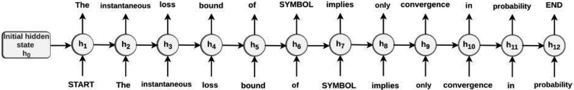
A generated sentence by indirect and direct RNN generators in (20) and (15), where the RNN architecture is displayed, in which sentence “The instantaneous loss bound of SYMBOL implies only convergence in probability” with topic “MISC” is consecutively generated by words, h_t is the hidden node of RNNs in (20) and (15), and h₀ is the initial hidden state, which is zero under (15) and “MISC” under (20).

On the ground of (15), the cost function L_m(θ_m) in (3) becomes

$$\begin{gathered} L_m\left({\theta }_m\right)=-{\left(n+\tilde{n}\right)}^{-1}\sum _{i=1}^n{\left(T^i\right)}^{-1}\sum _{t=1}^{T^i}\text{log}\left(o_{\left[x_{t+1}^i\right]}\left(x_t^i,h_t^i,{\theta }_m\right)\right) \\ -{\left(n+\tilde{n}\right)}^{-1}\sum _{j=1}^{\tilde{n}}{\left(T^j\right)}^{-1}\sum _{t=1}^{T^j}\text{log}\left(o_{\left[x_{t+1}^j\right]}\left(x_t^j,h_t^j,{\theta }_m\right)\right)+{\lambda }_m{J}_m\left({\theta }_m\right), \end{gathered}$$ (17)

where λ_m ≥ 0 is a tuning parameter and J_m(θ_m) is a regularizer regularizing the weights matrix and the activation layer [22].

Minimizing (14) and (17) yields estimators θ_b and θ_m, respectively. Then the conditional probabilities are estimated as $\widehat{p}\left(y\mid x_{1:t+1};{\theta }_b\right)=\sigma \left({\theta }_b\mathcal{E}\left(x_{1:t+1}\right)\right)$ and $\widehat{p}\left(x_{t+1}\mid x_{1:t};{\theta }_m\right)=o_{\left[x_{t+1}\right]}\left(x_t,h_{t-1},{\theta }_m\right)$. Plugging these estimates into (12), we obtain the estimated probability, and the process is summarized as,

$$\begin{gathered} {\widehat{p}}^b\left(X_{t+1}=x\mid x_{1:t},y\right)=\frac{\widehat{p}\left(y\mid x_{1:t},x;{\theta }_b\right)\widehat{p}\left(X_{t+1}=x\mid x_{1:t};{\theta }_m\right)}{\sum _{x\in \mathcal{D}}\widehat{p}\left(y\mid x_{1:t},x;{\theta }_b\right)\widehat{p}\left(X_{t+1}=x\mid x_{1:t};{\theta }_m\right)} \\ {\theta }_b=\underset{{\theta }_b}{\text{argmin}}{L}_b\left({\theta }_b\right),\hspace{1em}{\theta }_m=\underset{{\theta }_m}{\text{argmin}}{L}_m\left({\theta }_m\right). \end{gathered}$$ (18)

Then, a sentence is sequentially generated as follows:

$${\widehat{x}}_{t+1}=\underset{x\in \mathcal{D}}{\text{argmax}}{\widehat{p}}^b\left(X_{t+1}=x\mid X_{1:t}=x_{1:t},Y=y\right);t=1,\cdots ,\widehat{T}.$$ (19)

This generation process begins with x₁ = ``START″ or pre-specified t<sub>0</sub>-words $x_{1:t_0}$ and proceeds until $x_{\widehat{T}}=``\text{END}″$ is reached, where $\widehat{T}$ is an index at termination. It is worth mentioning that the denominator in (18) normalizes the probability but may not need to be computed when a maximizer of (18) is desired in (19).

4.2. Direct generator

The direct generation is inspired by a conditional RNN (C-RNN; [37, 17]) by estimating

$$p\left(x_{t+1}\mid x_{1:t},y\right)=o_{\left[x_{t+1}\right]}\left(x_t,h_{t-1},y,{\theta }_{\text{f}}\right),\text{with}{h}_t=h\left(x_t,h_{t-1},{\theta }_{\text{f}}\right),h_0=h_0\left(y,{\theta }_{\text{f}}\right),$$ (20)

where θ_f represents the parameters of a RNN, and h₀ is built on the label information as opposed to h₀ =0 in (16). As in (16), the direct generator requires additional parameters $W_{\text{f}}^y\in {ℝ}^{r_{\text{f}}\times K}$ for ${\theta }_{\text{f}}=\left(W_{\text{f}}^o,W_{\text{f}}^x,W_{\text{f}}^h,W_{\text{f}}^y\right)$ to model the effect from y as follows:

$$o\left(x_t,h_t,y,{\theta }_{\text{f}}\right)=\sigma \left(W_{\text{f}}^o{h}_t\right),h_t=\varphi \left(W_{\text{f}}^x{1}_{\left[x_t\right]}+W_{\text{f}}^h{h}_{t-1}\right),\text{and}{h}_0=\varphi \left(W_{\text{f}}^{y}y\right),$$ (21)

where $W_{\text{f}}^o\in {ℝ}^{r_{\text{f}}\times |\mathcal{D}|}$, $W_{\text{f}}^x\in {ℝ}^{|\mathcal{D}|\times r_{\text{f}}}$, $W_{\text{f}}^h\in {ℝ}^{r_m\times r_{\text{f}}}$, and r_f is the number of latent factors of the RNN. On this ground, the cost function in (4) becomes

$$L_{\text{f}}\left({\theta }_{\text{f}}\right)=-n^{-1}\sum _{i=1}^n{\left(T^i\right)}^{-1}\sum _{t=1}^{T_i}\text{log}\left(o_{\left[x_{t+1}^i\right]}\left(x_t^i,h_{t-1}^i,y^i,{\theta }_{\text{f}}\right)\right)+{\lambda }_{\text{f}}{J}_{\text{f}}\left({\theta }_{\text{f}}\right),$$ (22)

where λ_f ≥ 0 is a tuning parameter and J_f (θ_f) is a nonnegative regularizer. Minimizing (22) in θ_f yields an estimate θ_f, thus the estimated probability ${\widehat{p}}^{\text{f}}\left(x\mid x_{1:t},y\right)=o_{[x]}\left(x_t,h_{t-1},y,{\theta }_{\text{f}}\right)$, from (20). Then, sentence generation proceeds as in (19).

Worth of note is that the direct and indirect generators can be respectively implemented using different RNN models, for example, GPT2 for the direct RNN (20) while LSTM for the indirect RNN in (15). Moreover, different model architectures of RNNs may yield different empirical results. This aspect is illustrated in Section 5.

4.3. Coupled generator

Given the estimated probabilities ${\widehat{p}}^{\text{f}}\left(x_{t+1}\mid x_{1:t},y\right)$ and ${\widehat{p}}^b\left(x_{t+1}\mid x_{1:t},y\right)$. The coupled generator chooses one between ${\widehat{p}}^{\text{f}}$ and ${\widehat{p}}^b$ on a validation set by minimizing an empirical version of the log-likelihood loss,

$$\text{Ent}(\widehat{p})=-T^{-1}\sum _{t=1}^T\text{log}\widehat{p}\left(X_{t+1}=x_{t+1}\mid X_{1:t}=x_{1:t},Y=y\right).$$ (23)

4.4. Large-scale computation

This section develops a computational scheme for the indirect generator in (14)–(17), and the direct generator in (22) can be treated by a standard RNN implementation as in [36, 29]. In particular, when stochastic backpropagation is used through the time gradient method, the computation complexity is of order of the number of parameters per time step [27].

In what follows, we apply gradient descent [41] or stochastic gradient descent [31] to solve (14). For (17), we apply a classical back-propagation algorithm. In each case, we use analytic a gradient expression for updates.

Gradient for indirect generation.

The gradient expression for θ_m in (17) is given in [29], while that for θ_b in (14) is computed as

$$\frac{\partial L_b}{\partial {\theta }_{b,k}}=\{\begin{array}{ll}{\lambda }_b{\theta }_{b,k}-n^{-1}\sum _{i=1}^n{\left(T^i\right)}^{-1}\sum _{t=1}^{T^i}(y_k^i-{\sigma }_k\left({\theta }_b\mathcal{E}\left(x_{1:t}^i\right)\right)\mathcal{E}\left(x_{1:t}^i\right),\hfill & y^i\in {\{0,1\}}^K,\hfill \\ {\lambda }_b{\theta }_{b,k}-n^{-1}\sum _{i=1}^n{\left(T^i\right)}^{-1}\sum _{t=1}^{T^i}\left(y_k^i-{{\theta }^{\prime }}_{b,k}\mathcal{E}\left(x_{1:t}^i\right)\right)\mathcal{E}\left(x_{1:t}^i\right),\hfill & y^i\in {ℝ}^K,\hfill \end{array}$$ (24)

where θ_b,k denotes the kth column of θ_b.

The detail of gradient descent for the indirect generator is summarized as follows.

Algorithm 1 can be updated by a stochastic gradient scheme [2]. Lemma 1 describes computational properties of Algorithm 1.

Lemma 1.

If the cost functions L_b in (14) and L_m in (17) are continuously twice differential, and the probability measure of random initialization is absolutely continuous with respect to the Lebesgue measure. Then, θ_b is a global minimizer of (14), while θ_m is a local minimizer of (17) almost surely, provided that the step size in Algorithm 1 is sufficiently small.

4.5. Theory for sentence generation

This section generalizes the theoretical result of Section 3 to the problem of next-word-prediction.

Now we use p_X|Y, p_Y|X, and p_X to respectively represent ${\left\{p_{X_{t+1}\mid X_{1:t},Y}\right\}}_{t=1}^T,{\left\{p_{Y\mid X_{1:t}}\right\}}_{t=1}^T$, and ${\left\{p_{X_{t+1}\mid X_{1:t}}\right\}}_{t=1}^T$. The expected square Hellinger-distance for next-word-prediction is

$$d\left(p_{X\mid Y},q_{X\mid Y}\right)={\left(\overline{\mathbb{E}}{h}^2\left(p_{X_{t+1}\mid X_{1:t},Y},q_{X_{t+1}\mid X_{1:t},Y}\right)\right)}^{\frac{1}{2}},$$ (25)

where $\overline{\mathbb{E}}(\cdot )=T^{-1}\sum _{t=1}^T{\mathbb{E}}_{{\mathit{X}}_{1:t},\mathit{Y}}(\cdot )$.

The metric entropy of ${\mathcal{F}}_{b,k}$ is defined by a distance ${\kappa }^2\left(p_{Y\mid X},q_{Y\mid X}\right)=\overline{\mathbb{E}}{h}^2\left(p_{Y\mid X_{1:t}},q_{Y\mid X_{1:t}}\right)$. Similarly, ${\kappa }^2\left(p_X,q_X\right)=\overline{\mathbb{E}}{h}^2\left(p_{X_{t+1}\mid X_{1:t}},q_{X_{t+1}\mid X_{1:t}}\right)$, and d²(p_X|Y, q_X|Y) are used for ${\mathcal{F}}_{m,k}$ and ${\mathcal{F}}_{\text{f},k}$, respectively.

The approximation error for p_Y|X⁰ is ${\rho }_b\left({p_{Y\mid X}}^0,p_{Y\mid X}\right)=\overline{\mathbb{E}}{g}_{\alpha }\left(\frac{p^0\left(Y\mid X_{1:t+1}\right)}{p\left(Y\mid X_{1:t+1}\right)}\right)$. Similarly, the approximation errors ${\rho }_m\left({p_X}^0,p_X\right)=\overline{\mathbb{E}}{g}_{\alpha }\left(\frac{p^0\left(X_{t+1}\mid X_{1:t}\right)}{p\left(X_{t+1}\mid X_{1:t}\right)}\right)$ and ${\rho }_{\text{f}}\left({p_{X\mid Y}}^0,p_{X\mid Y}\right)=\overline{\mathbb{E}}{g}_{\alpha }\left(\frac{p^0\left(X_{t+1}\mid X_{1:t},Y\right)}{p\left(X_{t+1}\mid X_{1:t},Y\right)}\right)$ are used for p_X⁰ and p_X|Y⁰.

Corollary 1 (Sequential generation).

All the results in Theorems 1 and 2 continue to hold with the distance d(·,·) defined in (25).

Next we provide a theoretical example to illustrate Corollary 1.

Theoretical example.

Suppose that the RNN in (15) is a basic recurrent network with ${\theta }_m=\left(W_m^o,W_m^x,W_m^h\right)$, that is, $o\left(x_t,h_{t-1},{\theta }_m\right)=\sigma \left(W_m^o{h}_{t-1}\right),h_t=\varphi \left(W_m^x{1}_{\left[x_t\right]}+W_m^h{h}_{t-1}\right)$, and $h_0=0_{r_m}$, where $W_m^o\in {ℝ}^{r_m\times |\mathcal{D}|}$, $W_m^x\in {ℝ}^{|\mathcal{D}|\times r_m}$, and $W_m^h\in {ℝ}^{r_m\times r_m}$, r_m is the number of latent factors of the RNN, and ϕ(z) is an activation function, such as the sigmoid function ϕ(z) = 1/ (1+ exp(−z)), the tanh function ϕ(z) = tanh(z), and the Rectified linear unit (ReLU) ϕ(z) = z₊. For illustration, we focus on the sigmoid function.

The RNN in (20) is that $o\left(x_t,h_{t-1},{\theta }_{\text{f}}\right)=\sigma \left(W_{\text{f}}^o{h}_{t-1}\right)$, $h_t=\varphi \left(W_{\text{f}}^x{1}_{\left[x_t\right]}+W_{\text{f}}^h{h}_{t-1}\right)$, and $h_0=\varphi \left(W_{\text{f}}^{y}y\right)$. The network parameters are ${\theta }_{\text{f}}=\left(W_{\text{f}}^o,W_{\text{f}}^x,W_{\text{f}}^h,W_{\text{f}}^y\right)$, where $W_{\text{f}}^o\in {ℝ}^{r_{\text{f}}\times |\mathcal{D}|}$, $W_{\text{f}}^x\in {ℝ}^{|\mathcal{D}|\times r_{\text{f}}}$, $W_{\text{f}}^h\in {ℝ}^{r_{\text{f}}\times r_{\text{f}}}$, and $W_{\text{f}}^y\in {ℝ}^{r_{\text{f}}\times K}$, and r_f is the number of latent factors of the RNN in the direct generation.

Corollary 2 gives the generation errors of the direct and indirect generators.

Corollary 2 (Theoretical example).

For the estimated next-word probabilities $p_{X\mid Y}^{\text{f}}$ by the direct generator in (22), we have that $d\left(p_{X\mid Y}^{\text{f}},p_{X\mid Y}^0\right)=O_p\left({\eta }_{\text{f}}\right)$, where

$${\eta }_{\text{f}}=\text{max}\left\{{\left(\frac{{\Lambda }_{\text{f}}}{n}\text{log}\left(\frac{n\text{max}\left(r_{\text{f}},2c_{15}\right)2^T{T}^{-1/2}}{{\Lambda }_{\text{f}}}\right)\right)}^{\frac{1}{2}},{\gamma }_{\text{f}}^{\frac{1}{2}}\right\},$$

${\Lambda }_{\text{f}}=r_{\text{f}}\left(2|\mathcal{D}|+r_{\text{f}}+K\right)$, ${\lambda }_{\text{f}}=c_{17}{\eta }_{\text{f}}^2$, and c₁₅ > 0 and c₁₆ > 0 are constants with ${\mathbb{E}}_Y\Vert Y{\Vert }_2^2\le c_{15}$. Similarly, the estimated next-word probabilities $p_{X\mid Y}^b$ by the indirect generator in (14) and (17) satisfies: $d\left(p_{X\mid Y}^b,p_{X\mid Y}^0\right)=O_p\left({\eta }_b+{\eta }_m\right)$, where

$${\eta }_b=\text{max}\left\{{\left(\frac{{\Lambda }_b}{n}\text{log}\left(\frac{c_{16}n}{{\Lambda }_b}\right)\right)}^{\frac{1}{2}},{\gamma }_b^{\frac{1}{2}}\right\},$$

$${\eta }_m=\text{max}\left\{{\left(\frac{{\Lambda }_m}{n+\tilde{n}}\text{log}\left(\frac{r_m(n+\tilde{n})2^T{T}^{-1/2}}{{\Lambda }_m}\right)\right)}^{\frac{1}{2}},{\gamma }_m^{\frac{1}{2}}\right\},$$

Λ_b = Kp, ${\Lambda }_m=r_m\left(2|\mathcal{D}|+r_m\right)$, ${\lambda }_b=c_{18}{\eta }_b^2$, ${\lambda }_m=c_{18}{\eta }_m^2$, and c₁₆ > 0 and c₁₈ > 0 are constants with $\overline{\mathbb{E}}{\Vert \mathcal{E}\left(X_{1:t}\right)\Vert }_2^2\le c_{16}$.

Corollary 2 says that the generation error of the indirect generator in (1) becomes $d\left({{\widehat{p}}_{X\mid Y}}^b,{p_{X\mid Y}}^0\right)=O_p{\left(\frac{{\Lambda }_b}{n}\text{log}\left(\frac{n}{{\Lambda }_b}\right)\right)}^{\frac{1}{2}}$ when $(\tilde{n}+n)/n=O\left(\frac{{\Lambda }_m\text{log}\left(r_{m}n/{\Lambda }_m\right)}{{\Lambda }_b\text{log}\left(c_{16}n/{\Lambda }_b\right)}\right)$, when γ_b = γ_m = 0. In fact, the generation error is primarily dominated by its estimation error of p(Y | X_1:t), because p(X_t+1 | X_1:t) can be well estimated with the help of large unlabeled data with $\tilde{n}\gg n$. In this situation, the indirect method outperforms the direct method, particularly when Λ_b < Λ_f, suggesting that the estimation complexity of the indirect method is less than that of the direct method. Interestingly, the generation error of the direct generator agrees with that of the maximum likelihood estimates under the Hellinger-distance [34, 38]. With respect to tuning, a large value of Λ_b, Λ_m, and Λ_f increases the complexity of the corresponding functional space for probability estimation, thus reduces the generation errors. Consequently, the generation errors of the direct and indirect generators indeed depend on the model complexity of parameter spaces ${\mathcal{F}}_b$ and ${\mathcal{F}}_{\text{f}}$.

To illustrate the synergy of indirect and direct generators’ respective strengths, we consider two situations. First, $d\left(p_{X\mid Y}^{\text{f}},p_{X\mid Y}^0\right)=o_p(1)$ but $d\left(p_{X\mid Y}^b,p_{X\mid Y}^0\right)$ is bounded away from zero if an unlabeled sample ${\left(X_{1:T^j}^j\right)}_{j=1}^{\tilde{n}}$ follows a different marginal distribution of the labeled sample ${\left(X_{1:T^i}^i\right)}_{i=1}^n$. Second, $d\left(p_{X\mid Y}^b,p_{X\mid Y}^0\right)=o_p(1)$ but $d\left(p_{X\mid Y}^{\text{f}},p_{X\mid Y}^0\right)$ is bounded away from zero in the presence of a new word in labeled but unlabeled samples. However, in both situations, $d\left(p_{X\mid Y}^c,p_{X\mid Y}^0\right)=o_p(1)$, when Kullback-Leibler divergence is equivalent to the Hellinger-distance. In other words, only the coupled generator has a generation error tending to zero in both situations.

5. Benchmark

This section examines the performance of the coupled, indirect, and direct generators in one benchmark example, and compares with a baseline method “Separate RNN”, which fits RNNs for each topic as in [36]. The benchmark concerns sentence categorization based on a text corpus in the UCI machine learning repository². This corpus contains 1,039 labeled sentences collected from abstracts and introductions of 30 articles, in which five topic categories are AIM (a specific aim of the present paper), OWN (description of own work presented in the present paper), CONTRAST (comparison statements with other works, including strengths and weaknesses), BASIS (statements of agreement with other works or continuation of other works), and MISC (generally accepted scientific background or description of other works). These labels originate from three scientific domains: computational biology (PLOS), the machine learning repository on arXiv (ARXIV), and the psychology journal judgment and decision making (JDM). For example, a typical sentence such as “The instantaneous loss bound of SYMBOL implies only convergence in probability. ” is labeled as “MISC” according to scientific topic classification. In addition to the aforementioned labeled sentences, this corpus contains 34,481 unlabeled sentences from 300 articles in PLOS, ARXIV, and JDM.

Before proceeding, we pre-process the text corpus to filter out redundant each sentence’s component so that numerical embeddings are applied for the indirect generator. First, we replace all numerical values, symbolic values, and citations by “NUMBER”, “SYMBOL”, and “CITATION”, respectively, and remove all standalone punctuation marks except commas, periods, and semicolons. For unlabeled sentences, we remove words appearing less than 20 times in the corpus, which leads to an unlabeled corpus of 8,286 sentences. On this ground, a dictionary is constructed, consisting of 5,369 words extracted from labeled and unlabeled sentences.

For training, we generate word strings for next-word-prediction based on the maximum length of all sentences in the dataset. Thus, all the previous tokens in the sentence are contributing to predict the next word. Specifically, we create next-word-prediction sequences consisting of consecutive previous words and fill with the null word “NULL” to pad all word strings as the same length. An example of such a next-word-prediction sequence is displayed in Table 1. In this fashion, we gather enough training sentences as the null words do not impact our learning process. Now, 28,180 labeled next-word-prediction sequences are generated from the original 1,039 labeled sentences, together with 174,355 unlabeled sequences from the original 8,286 unlabeled sentences.

The generation performance is measured by two commonly used metrics, namely, the next-word entropy loss and the Bi-Lingual Evaluation Understudy (BLEU) loss [28] over a test sample, approximating the predicted Kullback-Leibler divergence and Jaccard distance [13], respectively. Given sentences ${\left(x_{1:{\widehat{T}}^i}^i\right)}_{i=1}^{n_{\text{test}}}$ generated from p and its reference sentence ${\left(x_{1:T^i}^i\right)}_{i=1}^{n_{\text{test}}}$ given a topic y, the entropy loss is defined in as the empirical version of (23), while the BLEU_l-loss (l =1, …, 4) can be written as

$${\text{BLEU}}_l-\text{loss}(p)=1-n_{\text{test}}^{-1}\sum _{i=1}^{n_{\text{test}}}\text{exp}\left(\text{min}\left(1-\frac{{\widehat{T}}^i}{T^i},0\right)\right)\frac{\left|{\text{gram}}_l\left(x_{1:T^i}^i\right)\cap {\text{gram}}_l\left(x_{1:{\widehat{T}}^i}^i\right)\right|}{\left|{\text{gram}}_l\left(x_{1:{\widehat{T}}^i}^i\right)\right|},$$

where n_test is the number of sentences in the testing set, |·| denotes a set’s size and gram_l(·) is the l-gram set for a sentence. For a sentence “the cat in the hat”, its 1-gram set is {“the”, “cat”, “in”, “the”, “hat”}, the 2-gram set is {“the cat”, “cat in”, “in the”, “the hat”}, and the 3-gram set is {“the cat in”, “cat in the”, “in the hat”}. The BLEU_l-loss can be computed using the NLTK library in Python. Whereas the entropy loss measures the occurrence probability of the reference sentences, the BLEU_l-loss focuses on exact matching between l consecutive words of two sentence. Moreover, we also consider the SF-BLEU_l-loss to evaluate the diversity of a generated sentences [43], defined as

$$\text{SF}-{\text{BLEU}}_l-\text{loss}(p)=1-n_{\text{test}}^{-1}\sum _{i=1}^{n_{\text{test}}}\text{exp}\left(\text{min}\left(1-\frac{{\widehat{T}}^i}{{\widehat{T}}_{\text{min}}^{-i}},0\right)\right)\frac{{\text{max}}_{j\ne i}\left|{\text{gram}}_l\left(x_{1:{\widehat{T}}^i}^i\right)\cap {\text{gram}}_l\left(x_{1:{\widehat{T}}^j}^j\right)\right|}{\left|{\text{gram}}_l\left(x_{1:{\widehat{T}}^i}^i\right)\right|},$$

where ${\widehat{T}}_{\text{min}}^{-i}=\underset{{\widehat{T}}^j;j\ne i}{\text{argmin}}\left|{\widehat{T}}^j-{\widehat{T}}^i\right|$, and a high SF-BLEU_l-loss score means more diverse.

For training, validation, and testing, we randomly split all the labeled articles into three sets with a partition ratio of 60%, 20%, and 20%, respectively. Moreover, for a sentence x_1:T and its associated topic y in a testing set, five starting words x_1:5 as opposed to the null word are given to predict the rest of a sentence.

Consider two situations of the semantic label: (1) Y ∈ {0, 1}^K is categorical and is coded as a 0–1 vector using the one-hot encoding from the topic category; (2) $Y\in {ℝ}^K$ is continuous with each topic as a p = 128-dimensional vector based on Doc2Vec. In (2), each topic is represented by the averaged embedding of all the sentences in this topic category in training data.

In the case of Y ∈ {0, 1}^K, the indirect generator involves (14) and (17). For (14), we perform regularized multinomial logistic regression using the Python library sklearn³ on the embedded next-word prediction sequence training samples $\left(\mathcal{E}\left(x_{1:t}^i\right),y^i\right)$, where $\mathcal{E}\left(x_{1:t}^i\right)$ is the numerical embedding of Doc2Vec⁴ of size p = 128 and the optimal λ_b is obtained by minimizing the entropy loss based on validation data over a set of grids {.0001, .001, .01, .1, 1, 10, 100}. For (17), the indirect RNN is trained based on both labeled and unlabeled next-word prediction sequences in training data. The indirect RNN model in (17) is structured in four layers, including an embedding layer consisting of 5, 369 nodes with each node corresponding one word in the dictionary $\mathcal{D}$, an LSTM layer of 128 latent factors, a dense layer with output dimension 5, 369. Note that the tuning parameter in (17) is fixed as λ_m = .0001 through in the embedding layer to regularize words in the absence in a training set. Similarly, the direct generator trains the RNN model in (22), which has the same configuration as the indirect RNN expect that the input dimension is $\left|\mathcal{D}\right|+K=5,374$ in its embedding layer. Moreover, Separate RNN has the same structure as the indirect RNN given each topic.

As discussed in Section 4.2, different RNN model architectures may yield different empirical performance. Toward this end, we compare the LSTM architecture with GPT2 architecture for the direct RNNs. In particular, we consider the base GPT2 with 12 layers and 117M parameters [30] for the direct method, denoted as direct-GPT2. One key difference between LSTM and GPT2 lies in its masked self-attention layer, which masks future tokens and passes the attention information through tokens that are positioned at the left of the current position.

In the case of continuous $Y\in {ℝ}^p$ after numerical embedding, the indirect generation proceeds as in the categorical case except that linear regression as opposed to multinomial logistic regression in (14) is performed using sklearn on the labeled embedded next-word prediction sequences in training data $\left(\mathcal{E}\left(x_{1:t}^i\right),y^i\right)$, where each yⁱ is a 128-dimensional embedding vector.

All RNN models are trained using Keras⁵ with the batch and epoch sizes 200 and 100, and optimizer as Adam, and the over-fitting is prevented by early termination [4] of patience as 20. Moreover, the coupled generator is tuned as in (5).

As indicated in Table 2, when only labeled data is available, the coupled generator delivery higher accuracy than direct and indirect generators, which suggests the advantage of the proposed method. When combining with unlabeled data, the coupled generator outperforms the direct generator and separate RNN for both categorical and continuous labels, which selects the indirect generator in this case. With respect to the entropy loss, the amounts of improvement of the indirect generator over the separate RNN method and direct generator are 20.3% and 14.5% for the categorical case and 29.1% and 16.1% for the continuous case. With respect to BLEU₁–BLEU₄ losses, a similar situation occurs, with the amounts of improvement vary with the best improvement around 15.6%. Concerning unlabeled data, a comparison between the indirect generator with and without unlabeled data suggests that unlabeled data indeed help to improve the performance of the indirect generation over 14.5%. Interestingly, in terms of the entropy loss, the direct generator based on fine-tuned GPT2 outperforms the direct generator and indirect generator based on LSTM without unlabeled data, while the coupled generator achieves the best performance between them. However, they perform similarly in terms of BLEU_l scores. In view of the SF-BLEU_l scores, sentences generated by the direct and indirect generators have a high degree of diversity. Moreover, the semantic label Y after sentence embeddings Doc2Vec performs slightly worse than its categorical counterpart for the indirect and direct generations, indicating that semantic relations or linguistics dependencies, as captured by the sentence embeddings, may not have an impact given that there are only five categories. Finally, as suggested in Table 3, an abstract generated based on the five categories is reasonable except for three grammatical errors that are correctable by a grammar checker⁶.

Table 2.

Test errors in loss functions–Entropy, BLEU_l, and SF-BLEU_l (standard errors in parentheses) of various generators based on 20 random partitions of the UCI sentence categorization text corpus. Here “Separate RNN”, “Indirect”, “Direct”, “Direct-GPT2” and “Coupled” denote the separate RNN, indirect, and direct generators based on the RNN-LSTM architecture, the direct generator based on the RNN-GPT architecture, and the coupled generator, while Indirect-label or Coupled-label refers to the generation without unlabeled data.

Method	Entropy	BLEU1-loss	BLEU2-loss	BLEU3-loss	BLEU4-loss
Y : categorical label
Separate RNN	9.317(.040)	0.895(.010)	0.926(.008)	0.954(.007)	0.971(.005)
Indirect	7.424(.049)	0.768(.003)	0.854(.002)	0.885(.002)	0.914(.002)
Indirect-label	8.839(.060)	0.831(.008)	0.878(.005)	0.899(.004)	0.923(.003)
Direct	9.537(.054)	0.823(.008)	0.872(.005)	0.895(.005)	0.919(.004)
Direct-GPT2	8.684(.051)	0.900(.006)	0.954(.002)	0.970(.001)	0.981(.001)
Coupled	7.424(.049)	0.768(.003)	0.854(.002)	0.885(.002)	0.914(.002)
Coupled-label	8.644(.050)	0.880(.008)	0.932(.008)	0.949(.007)	0.963(.006)
		SF-BLEU1-loss	SF-BLEU2-loss	SF-BLEU3-loss	SF-BLEU4-loss
Separate RNN		0.076(.010)	0.208(.027)	0.271(.036)	0.303(.043)
Method	Entropy	BLEU1-loss	BLEU2-loss	BLEU3-loss	BLEU4-loss
Indirect		0.105(.006)	0.296(.009)	0.416(.012)	0.502(.013)
Indirect-label		0.138(.008)	0.363(.022)	0.472(.029)	0.545(.036)
Direct		0.139(.006)	0.372(.019)	0.487(.026)	0.561(.032)
Direct-GPT2		0.053(.006)	0.159(.019)	0.255(.031)	0.320(.040)
Coupled		0.105(.006)	0.296(.009)	0.416(.012)	0.502(.013)
Coupled-label		0.082(.011)	0.233(.028)	0.342(.038)	0.417(.045)
Method	Entropy	BLEU1-loss	BLEU2-loss	BLEU3-loss	BLEU4-loss
Y: continuous label based on Doc2Vec [23, 24]
Indirect	7.641(.036)	0.768(.005)	0.851(.003)	0.883(.003)	0.912(.003)
Indirect-label	8.512(.041)	0.912(.010)	0.937(.008)	0.949(.007)	0.960(.005)
Direct	9.102(.050)	0.916(.010)	0.939(.007)	0.950(.005)	0.961(.004)
Coupled	7.641(.036)	0.768(.005)	0.851(.003)	0.883(.003)	0.912(.003)
Coupled-label	8.512(.041)	0.912(.010)	0.937(.008)	0.949(.007)	0.960(.005)
		SF-BLEU1-loss	SF-BLEU2-loss	SF-BLEU3-loss	SF-BLEU4-loss
Indirect		0.097(.005)	0.261(.008)	0.361(.010)	0.440(.012)
Method	Entropy	BLEU1-loss	BLEU2-loss	BLEU3-loss	BLEU4-loss
Indirect-labeled		0.064(.010)	0.165(.026)	0.211(.035)	0.232(.040)
Direct		0.079(.014)	0.202(.037)	0.252(.046)	0.271(.050)
Coupled		0.097(.005)	0.261(.008)	0.361(.010)	0.440(.012)
Coupled-label		0.064(.010)	0.165(.026)	0.211(.035)	0.232(.040)

Appendix

Proof of Lemma 1.

Note that L_b (θ_b) in (14) is convex in θ_b and L_b (θ_b) and L_m(θ_m) in (17) are continuously twice-differential. Then the result follows from Theorem 4 of [21]. This completes the proof. □

Proof of Theorem 1.

Note that ${\widehat{p}}_Y^b(y)=\int {\widehat{p}}_{Y\mid X}^b(y\mid x){\widehat{p}}_X^b(x)dx$ and

$$d^2\left({\widehat{p}}_{X\mid Y}^b,{p_{X\mid Y}}^0\right)=\int {\left({\left(\frac{p_Y^0(y){\widehat{p}}_{Y|X}^b(y\mid x){\widehat{p}}_X^b(x)}{{\widehat{p}}_Y^b(y)}\right)}^{1/2}-{\left(p_Y^0(y){p_{X\mid Y}}^0(x\mid y)\right)}^{1/2}\right)}^{2}dxdy.$$

Furthermore, $\int {\widehat{p}}_{Y\mid X}^b(y\mid x)dy=1$. It follows from the triangular inequality that

$$\begin{gathered} d\left({\widehat{p}}_{X|Y}^b,{p_{X\mid Y}}^0\right)\le {\left(\int {\left({\left(\frac{p_Y^0(y){\widehat{p}}_{Y|X}^b(y\mid x){\widehat{p}}_X^b(x)}{{\widehat{p}}_Y^b(y)}\right)}^{1/2}-{\left({\widehat{p}}_{Y|X}^b(y\mid x){\widehat{p}}_X^b(x)\right)}^{1/2}\right)}^{2}dxdy\right)}^{1/2} \\ +{\left(\int {\left({\left({\widehat{p}}_{Y\mid X}^b(y\mid x){\widehat{p}}_X^b(x)\right)}^{1/2}-{\left({\widehat{p}}_{Y\mid X}^b(y\mid x)p_X^0(x)\right)}^{1/2}\right)}^{2}dxdy\right)}^{1/2} \\ +{\left(\int {\left({\left({\widehat{p}}_{Y|X}^b(y\mid x)p_X^0(x)\right)}^{1/2}-{\left({p_{X|Y}}^0(x\mid y)p_X^0(x)\right)}^{1/2}\right)}^{2}dxdy\right)}^{1/2} \\ =h\left(p_Y^0,{\widehat{p}}_Y^b\right)+h\left(p_X^0,{\widehat{p}}_X^b\right)+{\left(\mathbb{E}\left(h^2\left({\widehat{p}}_{Y\mid X}^b,p_{Y\mid X}^0\right)\right)\right)}^{1/2}. \end{gathered}$$ (26)

Note that ${\widehat{p}}_{X,Y}^b(x,y)={\widehat{p}}_{Y\mid X}^b(y\mid x){\widehat{p}}_X^b(x)$. By the triangle inequality,

$$\begin{gathered} h\left(p_Y^0,{\widehat{p}}_Y^b\right)={\left(\int {\left({\left(\int p_{X,Y}^0(x,y)dx\right)}^{\frac{1}{2}}-{\left(\int {\widehat{p}}_{X,Y}^b(x,y)dx\right)}^{\frac{1}{2}}\right)}^{2}dy\right)}^{\frac{1}{2}} \\ \le {\left(\int {\left({\left(p_{X,Y}^0(x,y)\right)}^{\frac{1}{2}}-{\left({\widehat{p}}_{X,Y}^b(x,y)\right)}^{\frac{1}{2}}\right)}^{2}dxdy\right)}^{\frac{1}{2}} \\ \le {\left(\int {\left({\left(p_{X,Y}^0(x,y)\right)}^{\frac{1}{2}}-{\left(p_X^0(x){\widehat{p}}_{Y\mid X}^b(y\mid x)\right)}^{\frac{1}{2}}\right)}^{2}dxdy\right)}^{\frac{1}{2}} \\ +{\left(\int {\left({\left({\widehat{p}}_X^b(x)\right)}^{\frac{1}{2}}-{\left(p_X^0(x)\right)}^{\frac{1}{2}}\right)}^{2}dx\right)}^{\frac{1}{2}}\le h\left(p_X^0,{\widehat{p}}_X^b\right)+{\left(\mathbb{E}\left(h^2\left(p_{Y\mid X}^0,{\widehat{p}}_{Y\mid X}^b\right)\right)\right)}^{\frac{1}{2}}. \end{gathered}$$

Hence, $d\left({\widehat{p}}_{X\mid Y}^b,{p_{X\mid Y}}^0\right)\le 2\left(h\left({\widehat{p}}_X^b,p_X^0\right)+{\left(\mathbb{E}\left(h^2\left({\widehat{p}}_{Y\mid X}^b,p_{Y\mid X}^0\right)\right)\right)}^{1/2}\right)$. Consequently,

$$\begin{gathered} P\left(d\left({\widehat{p}}_{X\mid Y}^b,{p_{X\mid Y}}^0\right)\ge 2\left({\eta }_b+{\eta }_m\right)\right) \\ \le P\left(h\left(p_X^0,{\widehat{p}}_X\right)\ge {\eta }_m\right)+P\left({\left({\mathbb{E}}_X\left(h^2\left(p_{Y\mid X}^0,{\widehat{p}}_{Y\mid X}\right)\right)\right)}^{\frac{1}{2}}\ge {\eta }_b\right)\equiv I_1+I_2. \end{gathered}$$

To bound I₁, let

$$I_3=P\left({(n+\tilde{n})}^{-1}\sum _{i=1}^{n+\tilde{n}}\left(\text{log}\left(p_X^0\left(X^i\right)\right)-\text{log}\left(p_X^{*}\left(X^i\right)\right)\right)+{\lambda }_{m}J\left(p_X^0\right)+{\lambda }_{m}J\left(p_X^{*}\right)\right)\ge c_9{\eta }_m^2/4);$$

$$I_4=P(\underset{d_m\left(p,p^0\right)\ge {\eta }_m}{\text{sup}}{(n+\tilde{n})}^{-1}\sum _{i=1}^{n+\tilde{n}}\left(\text{log}\left(\frac{p_X\left(X^i\right)}{p_X^0\left(X^i\right)}-{\lambda }_{m}J\left(p_X\right)+{\lambda }_{m}J\left(p_X^0\right)\right)\ge -c_9{\eta }_m^2/4\right),$$

where c₉ 1 − 2exp(−τ / 2) / (1 − exp(−τ / 2))² > 0 is a constant defined by the truncation constant τ > 0. Then I₁ is upper bounded by

$$P\left(\underset{d_m\left(p,p^0\right)\ge {\eta }_m}{\text{sup}}{(n+\tilde{n})}^{-1}\sum _{i=1}^{n+\tilde{n}}\left(\text{log}\left(p_X\left(X^i\right)/p_X^{*}\left(X^i\right)\right)\right)-{\lambda }_{m}J\left(p_X\right)+{\lambda }_{m}J\left(p_X^{*}\right)\right)\ge 0)\le I_3+I_4.$$

By the Markov inequality,

$$\begin{gathered} I_3\le P\left({(n+\tilde{n})}^{-1}\sum _{i=1}^{n+\tilde{n}}\left(\text{log}\left(p_X^0\left(X^i\right)\right)-\text{log}\left(p_X^{*}\left(X^i\right)\right)\right)\ge c_9{\eta }_m^2/4-{\lambda }_{m}J\left(p_X^{*}\right)\right) \\ \le \prod _{i=1}^{n+\tilde{n}}{\mathbb{E}}_X{\left(\frac{p_X^0\left(X^i\right)}{p_X^{*}\left(X^i\right)}\right)}^{\alpha }\text{exp}\left(-\frac{c_9\alpha }{8}(n+\tilde{n}){\eta }_m^2\right) \\ \le {\left(1+\alpha {\gamma }_m\right)}^{n+\tilde{n}}\text{exp}\left(-\frac{c_9\alpha }{8}(n+\tilde{n}){\eta }_m^2\right)\le \text{exp}\left(-\frac{c_9\alpha }{8}(n+\tilde{n}){\eta }_m^2+(n+\tilde{n})\alpha {\gamma }_m\right). \end{gathered}$$

By Corollary 1 of [33], $I_4\le 7\text{exp}\left(-c_8(n+\tilde{n}){\eta }_m^2/2\right)$, implying $I_1\le 7\text{exp}\left(-c_7(n+\tilde{n}){\eta }_m^2\right)+\text{exp}\left(-\frac{c_9\alpha }{8}(n+\tilde{n}){\eta }_m^2+(n+\tilde{n})\alpha {\gamma }_m\right)$ for some constant c₇ > 0. For I₂, a similar probabilistic bound can be established by applying the same argument of Theorem 2 and switching the role of X and Y. This leads to $I_2\le 7\text{exp}\left(-c_{8}n{\eta }_b^2\right)+\text{exp}\left(-\frac{c_9\alpha }{8}n{\eta }_b^2+n\alpha {\gamma }_b\right)$ for some constant c₈ > 0. The desired result then follows. □

Proof of Theorem 2.

Denote

$$I_5=P\left(\underset{d\left(p,p^0\right)\ge {\eta }_{\text{f}}}{\text{sup}}\left(n^{-1}\sum _{i=1}^n\left(\text{log}\left(\frac{{p_{X\mid Y}}^{(\tau )}\left(X^i\mid Y^i\right)}{{p_{X\mid Y}}^{*}\left(X^i\mid Y^i\right)}\right)\right)-\lambda J\left(p_{X|Y}\right)+\lambda J\left({p_{X\mid Y}}^{*}\right)\right)\ge 0\right),$$

$$I_6=P\left(n^{-1}\sum _{i=1}^n\left(\text{log}\left(\frac{{p_{X\mid Y}}^0\left(X^i\mid Y^i\right)}{{p_{X\mid Y}}^{*}\left(X^i\mid Y^i\right)}\right)\right)-\lambda J\left({p_{X\mid Y}}^0\right)+\lambda J\left({p_{X\mid Y}}^{*}\right)\ge c_9{\eta }_{\text{f}}^2/4\right).$$

By the definition of a minimizer, for any η_f > 0,

$$P\left(d\left({\widehat{p}}_{X\mid Y}^{\text{f}},{p_{X\mid Y}}^0\right)\ge {\eta }_{\text{f}}\right)\le I_5+I_6,$$

where $\text{log}\left({\mathbb{F}}_i^{(\tau )}\right)=\text{log}\left({p_{X\mid Y}}^{(\tau )}\left(X^i\mid Y^i\right)\right)-\text{log}\left({p_{X\mid Y}}^0\left(X^i\mid Y^i\right)\right)$ and

$${p_{X\mid Y}}^{(\tau )}(x\mid y)=\{\begin{array}{ll}\text{exp}(-\tau ){p_{X\mid Y}}^{*}(x\mid y),\hfill & \text{ if }{p}_{X\mid Y}(x\mid y)<\text{exp}(-\tau ){p_{X\mid Y}}^{*}(x\mid y),\hfill \\ p_{X\mid Y}(x\mid y),\hfill & \text{ otherwise, }\hfill \end{array}$$

is the left truncation of p_X|Y(x|y).

Next, we bound I₅ and I₆ separately. An application of the same argument as in [38] yields that

$$\begin{gathered} I_5\le P\left(n^{-1}\sum _{i=1}^n\left(\text{log}\left({p_{X\mid Y}}^0\left(X^i\mid Y^i\right)\right)-\text{log}\left({p_{X\mid Y}}^{*}\left(X^i\mid Y^i\right)\right)\right)\ge c_9{\eta }_{\text{f}}^2/4-{\lambda }_{\text{f}}J\left({p_{X\mid Y}}^{*}\right)\right) \\ \le P\left(\prod _{i=1}^n{\left(\frac{{p_{X\mid Y}}^0\left(X^i\mid Y^i\right)}{{p_{X\mid Y}}^{*}\left(X^i\mid Y^i\right)}\right)}^{\alpha }\ge \text{exp}\left(\frac{c_9\alpha }{8}n{\eta }_{\text{f}}^2\right)\right) \\ \le \prod _{i=1}^n{\mathbb{E}}_Y{\mathbb{E}}_{X\mid Y}{\left(\frac{{p_{X\mid Y}}^0\left(X^i\mid Y^i\right)}{{p_{X\mid Y}}^{*}\left(X^i\mid Y^i\right)}\right)}^{\alpha }\text{exp}\left(-\frac{c_9\alpha }{8}n{\eta }_{\text{f}}^2\right)\le {\left(1+\alpha {\gamma }_{\text{f}}\right)}^n\text{exp}\left(-\frac{c_9\alpha }{8}n{\eta }_{\text{f}}^2\right) \\ \le \text{exp}\left(-\frac{\alpha }{8}{c}_{9}n{\eta }_{\text{f}}^2+n\text{log}\left(1+\alpha {\gamma }_{\text{f}}\right)\right)\le \text{exp}\left(-\frac{\alpha }{8}{c}_{9}n{\eta }_{\text{f}}^2+n\alpha {\gamma }_{\text{f}}\right), \end{gathered}$$ (27)

where the second inequality follows from ${\lambda }_{\text{f}}J\left({p_{X\mid Y}}^{*}\right)\le c_9{\eta }_{\text{f}}^2/8$ and the third inequality follows from Markov’s inequality.

Our treatment of bounding I₆ relies on a chaining argument over a suitable partition of ${\mathcal{F}}_{\text{f}}$ and the left-truncation of likelihood ratios as in [38, 33]. Now, consider a partition of ${\mathcal{F}}_{\text{f}}={\cup }_{k=1}^{\infty }{\cup }_{j=0}^{\infty }{\mathcal{F}}_{kj}$:

$${\mathcal{F}}_{kj}=\left\{p\in {\mathcal{F}}_{\text{f}}:2^{i-1}{\eta }_n^2\le d^2\left(p^0,p\right)\le 2^i{\eta }_n^2,2^{j-1}{J}^0\le J(p)\le 2^{j}J\left(p^0\right)\right\},$$

$${\mathcal{F}}_{k0}=\left\{p\in {\mathcal{F}}_{\text{f}}:2^{i-1}{\eta }_n^2\le d^2\left(p^0,p\right)\le 2^i{\eta }_n^2,J(p)\le J\left(p^0\right)\right\};k=1,\cdots ,j=0,\cdots ,$$

where $\text{log}\left({\mathbb{F}}_i^{(\tau )}\right)=\text{log}\left({p_{X\mid Y}}^{(\tau )}\left(X^i\mid Y^i\right)\right)-\text{log}\left({p_{X\mid Y}}^0\left(X^i\mid Y^i\right)\right)$. Then for any η_f > 0,

$$\begin{gathered} I_6\le P\left(\underset{d\left(p,p^0\right)\ge {\eta }_{\text{f}}}{\text{sup}}\left(n^{-1}\sum _{i=1}^n\text{log}\left({\mathbb{F}}_i^{(\tau )}\right)-{\lambda }_{\text{f}}J\left(p_{X\mid Y}\right)+{\lambda }_{\text{f}}J\left({p_{X\mid Y}}^0\right)\right)\ge -c_9{\eta }_{\text{f}}^2/4\right) \\ \le \sum _{k=1}^{\infty }\sum _{j=0}^{\infty }P\left(\underset{p\in {\mathcal{F}}_{kj}}{\text{sup}}\left(n^{-1}\sum _{i=1}^n\text{log}\left({\mathbb{F}}_i^{(\tau )}\right)-{\lambda }_{\text{f}}J\left(p_{X\mid Y}\right)+{\lambda }_{\text{f}}J\left({p_{X\mid Y}}^0\right)\right)\ge -c_9{\eta }_{\text{f}}^2/4\right) \\ \equiv \sum _{k=1}^{\infty }\sum _{j=0}^{\infty }{I}_{kj}, \end{gathered}$$ (28)

where $I_{kj}=P\left(\underset{f\in {\mathcal{F}}_{kj}}{\text{sup}}\left(n^{-1}\sum _{i=1}^n\text{log}\left({\mathbb{F}}_i^{(t)}\right)-{\lambda }_{\text{f}}J\left(p_{X|Y}\right)+{\lambda }_{\text{f}}J\left({p_{X\mid Y}}^0\right)\right)\ge -c_9{\eta }_{\text{f}}^2/4\right)$. To treat I_kj, we control the mean and variance of $\text{log}\left({\mathbb{F}}^{(\tau )}\right)$. By Lemma 4 of [38],

$$-\underset{p\in {\mathcal{F}}_{kj}}{\text{sup}}\mathbb{E}\left(\text{log}\left({\mathbb{F}}^{(\tau )}\right)\right)=-\underset{p\in {\mathcal{F}}_{kj}}{\text{sup}}{\mathbb{E}}_Y\left({\mathbb{E}}_{X\mid Y}\left(\text{log}\left({\mathbb{F}}^{(\tau )}\right)\right)\right)\ge c_9\underset{p\in {\mathcal{F}}_{kj}}{\text{inf}}{d}^2\left(p,p^{*}\right)\ge c_9{\left(2^{k-1}{\eta }_{\text{f}}\right)}^2,$$ (29)

and the variance is bounded by

$$\begin{gathered} \underset{p\in {\mathcal{F}}_{kj}}{\text{sup}}\text{Var}\left(\text{log}\left({\mathbb{F}}^{(\tau )}\right)\right)\le \underset{p\in {\mathcal{F}}_{kj}}{\text{sup}}{\mathbb{E}}_Y\left({\mathbb{E}}_{X\mid Y}\left(\text{log}{\left({\mathbb{F}}^{(\tau )}\right)}^2\right)\right) \\ \le 4\text{exp}(\tau )\underset{p\in {\mathcal{F}}_{kj}}{\text{sup}}{\mathbb{E}}_Y{h}^2\left(p_{X\mid Y}^0,p_{X\mid Y}\right)\le 4\text{exp}(\tau ){\left(2^k{\eta }_{\text{f}}\right)}^2\le 8\text{exp}(\tau ){\delta }_{kj}/c_9, \end{gathered}$$ (30)

where the second inequality follows from Lemma 3 of [38]. Then, I_kj is upper-bounded by

$$\begin{gathered} I_{kj}\le P(\underset{f\in {\mathcal{F}}_{kj}}{\text{sup}}\left(n^{-1}\sum _{i=1}^n\text{log}\left({\mathbb{F}}_i^{(\tau )}\right)-\mathbb{E}\text{log}\left({\mathbb{F}}^{(\tau )}\right)\right) \\ \ge -\underset{f\in {\mathcal{F}}_{kj}}{\text{sup}}\left(\mathbb{E}\text{log}\left({\mathbb{F}}^{(\tau )}\right)+\lambda \left(J\left({p_{X\mid Y}}^0\right)-J\left(p_{X\mid Y}\right)\right)\right)-c_9{\eta }_{\text{f}}^2/4) \\ \le P\left(\underset{f\in {\mathcal{F}}_{kj}}{\text{sup}}\left(n^{-1}\sum _{i=1}^n\text{log}\left({\mathbb{F}}_i^{(\tau )}\right)-\mathbb{E}\text{log}\left({\mathbb{F}}^{(\tau )}\right)\right)\ge {\delta }_{kj}\right)\le 3\text{exp}\left(-a_{3}n{\delta }_{kj}\right), \end{gathered}$$ (31)

where a₃ > 0 is a constant, ${\delta }_{kj}=c_9{2}^{k-1}{\eta }_n^2/2+\lambda \left(2^{j-1}-1\right)J\left({p_{X\mid Y}}^0\right)$, ${\delta }_{k0}=c_9{2}^{k-2}{\eta }_n^2/2$, the second inequality follows from the assumption that $\lambda J\left({p_{X\mid Y}}^0\right)\le c_9{\eta }_{\text{f}}^2/4$ and (29), and the last inequality follows from Lemma 2 and the fact that the j-th (j ≥ 2) moment $\mathbb{E}\left({\left|\text{log}\left(\frac{{p_{X\mid Y}}^{(\tau )}(X\mid Y)}{{p_{X\mid Y}}^0(X\mid Y)}\right)\right|}^j\right)$ is bounded by

$$\begin{gathered} {\mathbb{E}}_Y{\mathbb{E}}_{X\mid Y}\left(\text{exp}\left(\left|\text{log}\left(\frac{{p_{X\mid Y}}^{(\tau )}(X\mid Y)}{{p_{X\mid Y}}^0(X\mid Y)}\right)\right|\right)-1-\frac{1}{2}\left|\text{log}\left(\frac{{p_{X\mid Y}}^{(\tau )}(X\mid Y)}{{p_{X\mid Y}}^0(X\mid Y)}\right)\right|\right) \\ \le j!2^j{a}_1{\mathbb{E}}_Y{\Vert {\left(p_{X|Y}\right)}^{1/2}-{\left({p_{X\mid Y}}^0\right)}^{1/2}\Vert }_2^2, \end{gathered}$$

where a₁ =(exp(τ / 2) − 1 – τ / 2)/(1 − exp(−τ/2))² > 0 is a constant and the last inequality follows from Lemma 5 in [34]. It suffices to verify the condition (2.4) of [38]. A combination of (28) and (31) yield that $I_6\le \sum _{k=1}^{\infty }\sum _{j=0}^{\infty }3\text{exp}\left(-c_{13}n{\delta }_{kj}^2\right)\le 7\text{exp}\left(-c_{13}n{\eta }_{\text{f}}^2\right)$, which, together with (27) yields that $P\left(d\left({\widehat{p}}_{X\mid Y}^{\text{f}},{p_{X\mid Y}}^0\right)\ge {\eta }_{\text{f}}\right)\le I_5+I_6\le 7\text{exp}\left(-c_{13}n{\eta }_{\text{f}}^2\right)+\text{exp}\left(-\frac{\alpha }{8}{c}_{9}n{\eta }_{\text{f}}^2+n\alpha {\gamma }_{\text{f}}\right)$. The desired result then follows. □

Proof of Theorem 3.

Let ${\left(X^i,Y^i\right)}_{i=1}^N$ be a cross-validation sample. By (5),

$$-\frac{1}{N}\sum _{i=1}^N\text{log}{\widehat{p}}_{X|Y}^c\left(X^i\mid Y^i\right)\le \text{min}\left(-\frac{1}{N}\sum _{i=1}^N\text{log}{\widehat{p}}_{X|Y}^{\text{f}}\left(X^i\mid Y^i\right),-\frac{1}{N}\sum _{i=1}^N\text{log}{\widehat{p}}_{X|Y}^b\left(X^i\mid Y^i\right)\right),$$

then the desired result follows from the law of large number, by taking the limit for both the sides as N → ∞. This completes the proof. □

Proof of Corollary 1.

For the direct sequential generation, we apply the same argument in the proof of Theorem 2. Denote

$$I_7=P\left(\underset{d\left(p,p^0\right)\ge {\eta }_{\text{f}}}{\text{sup}}\sum _{i=1}^n\frac{1}{nT}\sum _{t=1}^T\text{log}\left(\frac{p^0\left(X_{t+1}^i\mid X_{1:t}^i,Y^i\right)}{p^{*}\left(X_{t+1}^i\mid X_{1t;}^i,Y^i\right)}\right)-{\lambda }_{\text{f}}{J}_{\text{f}}\left({p_{X\mid Y}}^0\right)+{\lambda }_{\text{f}}{J}_{\text{f}}\left({p_{X\mid Y}}^{*}\right)\ge \frac{c_9{\eta }_{\text{f}}^2}{4}\right),$$

$$I_8=P\left(\underset{d\left(p,p^0\right)\ge {\eta }_{\text{f}}}{\text{sup}}\sum _{i=1}^n\frac{1}{nT}\sum _{t=1}^T\text{log}\left(\frac{p^{(t)}\left(X_{t+1}^i\mid X_{1:t}^i,Y^i\right)}{p^0\left(X_{t+1}^i\mid X_{1:t}^i,Y^i\right)}\right)-{\lambda }_{\text{f}}{J}_{\text{f}}\left(p_{X\mid Y}\right)+{\lambda }_{\text{f}}{J}_{\text{f}}\left({p_{X\mid Y}}^0\right)\ge -\frac{c_9{\eta }_{\text{f}}^2}{4}\right).$$

Then $P\left(d\left(p_{X\mid Y}^{\text{f}},p_{X\mid Y}^0\right)\ge {\eta }_{\text{f}}\right)\le I_7+I_8$, where p^(τ) (X_t+1 | X_1:t, Y) is the left truncation of p(X_t+1 | X_1:t, Y) as defined in the proof of Theorem 2.

For I₇,

$$\begin{gathered} I_7\le P\left(\prod _{i=1}^n{\left(\prod _{t=1}^T\frac{p^0\left(X_{t+1}^i\mid X_{1:t}^i,Y^i\right)}{p^{*}\left(X_{t+1}^i\mid X_{1:t}^i,Y^i\right)}\right)}^{\frac{\alpha }{T-1}}\ge \text{exp}\left(\frac{c_9\alpha }{8}n{\eta }_{\text{f}}^2\right)\right) \\ \le \prod _{i=1}^n\mathbb{E}{\left(\prod _{t=1}^T\frac{p^0\left(X_{t+1}^i\mid X_{1:t}^i,Y^i\right)}{p^{*}\left(X_{t+1}^i\mid X_{1:t}^i,Y^i\right)}\right)}^{\frac{\alpha }{T-1}}\text{exp}\left(-\frac{c_9\alpha }{8}n{\eta }_{\text{f}}^2\right) \\ \le \prod _{i=1}^n\overline{\mathbb{E}}\left({\left(\frac{p^0\left(X_{t+1}^i\mid X_{1:t}^i,Y^i\right)}{p^{*}\left(X_{t+1}^i\mid X_{1:t}^i,Y^i\right)}\right)}^{\alpha }\right)\text{exp}\left(-\frac{c_9\alpha }{8}n{\eta }_{\text{f}}^2\right) \\ \le {\left(1+\alpha {\gamma }_{\text{f}}\right)}^n\text{exp}\left(-\frac{c_9\alpha }{8}n{\eta }_{\text{f}}^2\right)\le \overline{r}\text{exp}\left(-\frac{\alpha }{8}{c}_{9}n{\eta }_{\text{f}}^2+n\alpha {\gamma }_{\text{f}}\right). \end{gathered}$$

For I₈, let ${\mathbb{F}}_t^{(\tau )}=\text{log}\left(p^{(\tau )}\left(X_{t+1}\mid X_{1:t},Y\right)/p^0\left(X_{t+1}\mid X_{1:t},Y\right)\right)$. For the first moment,

$$\begin{gathered} \mathbb{E}\left(T^{-1}\sum _{t=1}^T{\mathbb{F}}_t^{(\tau )}\right)=T^{-1}\sum _{t=1}^T{\mathbb{E}}_{{\mathit{X}}_{1:t},\mathit{Y}}\left({\mathbb{E}}_{X_{t+1}}\left({\mathbb{F}}_t^{(\tau )}\mid X_{1:t},Y\right)\right) \\ \le -c_9{T}^{-1}\sum _{t=1}^T{\mathbb{E}}_{X_{1:t},Y}\left({\Vert {\left(p_{X_{t+1}\mid X_{1:t},Y}^{(\tau )}\right)}^{\frac{1}{2}}-{\left(p_{X_{t+1}\mid X_{1:t},Y}^0\right)}^{\frac{1}{2}}\Vert }_2^2\right)=-c_9{d}^2\left(p_{X\mid Y}^{(\tau )},p_{X\mid Y}^0\right). \end{gathered}$$

For the j-th moment with j ≥ 2,

$$\begin{gathered} \mathbb{E}{\left|T^{-1}\sum _{t=1}^T{\mathbb{F}}_t^{(\tau )}\right|}^j\le T^{-1}\sum _{t=1}^T{\mathbb{E}}_{X_{1:t},Y}\left({\mathbb{E}}_{X_{t+1}}\left({\left|{\mathbb{F}}_t^{(\tau )}\right|}^j\mid X_{1:t},Y\right)\right) \\ \le j!2^j{T}^{-1}\sum _{t=1}^T{\mathbb{E}}_{X_{1:t},Y}\left({\mathbb{E}}_{X_{t+1}}\left(\left(\text{exp}\left(\left|{\mathbb{F}}_t^{(\tau )}\right|/2\right)-1-\left|{\mathbb{F}}_t^{(\tau )}\right|/2\right)\mid X_{1:t},Y\right)\right) \\ \le j!2^j{a}_3\left(\sum _{t=1}^T{\mathbb{E}}_{X_{1:t},Y}\left({\Vert {\left(p_{X_{t+1}\mid X_{1:t},Y}^{(\tau )}\right)}^{\frac{1}{2}}-{\left(p_{X_{t+1}\mid X_{1:t},Y}^0\right)}^{\frac{1}{2}}\Vert }_2^2\right)\right) \\ \le j!2^j{a}_1{d}^2\left(p_{X\mid Y}^{(\tau )},p_{X\mid Y}^0\right), \end{gathered}$$

where the first inequality follows from the Jensen’s inequality. Then

$$P\left(d\left(p_{X\mid Y}^{\text{f}},p_{X\mid Y}^0\right)\ge {\eta }_{\text{f}}\right)\le 6\text{exp}\left(-c_{7}n{\eta }_{\text{f}}^2\right)+\text{exp}\left(-\frac{\alpha }{8}{c}_{9}n{\eta }_{\text{f}}^2+n\alpha {\gamma }_{\text{f}}\right),$$ (32)

follows the same arguments as in the proof of Theorem 2.

For the indirect generation, let p_t (·) = p(·| X_1:t) and ${\mathbb{E}}_t(\cdot )=\mathbb{E}\left(\cdot \mid X_{1:t}\right)$. Then,

$$\begin{gathered} d\left(p_{X\mid Y}^b,p_{X\mid Y}^0\right)={\left(T^{-1}\sum _{t=1}^T{\mathbb{E}}_{X_{1:t}}{\mathbb{E}}_{Y\mid X_{1:t}}{h}^2\left({\widehat{p}}_{X_{t+1}\mid X_{1:t},Y}^b,p_{X_{t+1}\mid X_{1:t},Y}^0\right)\right)}^{\frac{1}{2}} \\ \le 2(T^{-1}\sum _{t=1}^T{\left(\mathbb{E}\left(h\left({\widehat{p}}_{X_{t+1}\mid {\mathit{X}}_{1:t}},p_{X_{t+1}\mid {\mathit{X}}_{1:t}}^0\right)+{\left({\mathbb{E}}_t{h}^2{\left({\widehat{p}}_{\mathit{Y}\mid {\mathit{X}}_{1:t+1}},p_{\mathit{Y}\mid {\mathit{X}}_{1:t+1}}^0\right))}^{\frac{1}{2}}\right)}^2\right)\right)}^{\frac{1}{2}} \\ \le 2{\left(2T^{-1}\sum _{t=1}^T\left(\mathbb{E}{h}^2\left({\widehat{p}}_{X_{t+1}{|}_{X_{1:t}}},p_{X_{t+1}\mid X_{1:t}}^0\right)+\mathbb{E}{h}^2\left({\widehat{p}}_{Y\mid X_{1:t+1}},p_{Y\mid X_{1:t+1}}^0\right)\right)\right)}^{\frac{1}{2}} \\ \le 2\sqrt{2}\left(d\left(\widehat{p_X,p_X^0}\right)+d\left(\widehat{p_{Y\mid X}},p_{Y\mid X}^0\right)\right), \end{gathered}$$

where the first inequality follows from (26) by replacing p(·) as p_t (·), and $d^2\left(p_X,p_X^0\right)=\overline{\mathbb{E}}{h}^2\left({\widehat{p}}_{X_{t+1}\mid X_{1:t}},p_{X_{t+1}\mid {\mathit{X}}_{1:t}}^0\right)$, $d^2\left(p_{Y\mid X},p_{Y\mid X}^0\right)=\overline{\mathbb{E}}{h}^2\left({\widehat{p}}_{Y\mid X_{1:t+1}},p_{Y\mid X_{1:t+1}}^0\right)$. Therefore,

$$\begin{gathered} P\left(d\left(p_{X|Y}^b,p_{X|Y}^0\right)\ge 2\sqrt{2}\left({\eta }_b+{\eta }_m\right)\right)\le P\left(d\left(p_X,p_X^0\right)\ge {\eta }_m\right)+P\left(d\left(p_{Y|X},p_{Y\mid X}^0\right)\ge {\eta }_b\right) \\ \le 7\text{exp}\left(-c_7(n+\tilde{n}){\eta }_m^2\right)+\text{exp}\left(-\frac{\alpha c_9}{8}(n+\tilde{n}){\eta }_m^2+\alpha (n+\tilde{n}){\gamma }_m\right) \\ +7\text{exp}\left(-c_{8}n{\eta }_b^2\right)+\text{exp}\left(-\frac{\alpha c_9}{8}n{\eta }_b^2+\alpha n{\gamma }_b\right), \end{gathered}$$

where the last inequality follows from (32). Similarly, bounds for $P\left(d\left(p_X,p_X^0\right)\ge {\eta }_m\right)$ and $d\left(p_{Y\mid X},p_{Y\mid X}^0\right)$ can be established. The desired result then follows. □

Proof of Corollary 2.

It suffices to verify the entropy conditions in Corollary 1. For the direct generation, let $p_{X\mid Y}={\left\{p\left(X_{t+1}\mid X_{1:t},Y;{\theta }_{\text{f}}\right)\right\}}_{t=1}^T$ and ${\overline{p}}_{X\mid Y}={\left\{p\left(X_{t+1}\mid X_{1:t},Y;{\overline{\theta }}_{\text{f}}\right)\right\}}_{t=1}^T$ in ${\mathcal{F}}_{\text{f},k}$. Then

$$\begin{gathered} {\kappa }^2\left(p_{X\mid Y},{\overline{p}}_{X\mid Y}\right)\le \overline{\mathbb{E}}{\Vert {\sigma }^{\frac{1}{2}}\left(W_{\text{f}}^o{h}_{t-1}\right)-{\sigma }^{\frac{1}{2}}\left({\overline{W}}_{\text{f}}^o{\overline{h}}_{t-1}\right)\Vert }_2^2 \\ \le \frac{1}{2}\overline{\mathbb{E}}\left|\right|W_{\text{f}}^o{h}_{t-1}-{\overline{W}}_{\text{f}}^o{\overline{h}}_{t-1}|{|}_2^2 \\ \le \overline{\mathbb{E}}\left(\left|\right|\left(W_{\text{f}}^o-{\overline{W}}_{\text{f}}^o\right)h_{t-1}|{|}_2^2+|\left|{\overline{W}}_{\text{f}}^o\left(h_{t-1}-{\overline{h}}_{t-1}\right)\right|{|}_2^2\right) \\ \le \overline{\mathbb{E}}\left({\Vert W_{\text{f}}^o-{\overline{W}}_{\text{f}}^o\Vert }_F^2{\Vert h_{t-1}\Vert }_2^2+{\Vert {\overline{W}}_{\text{f}}^o\Vert }_F^2{\Vert h_{t-1}-{\overline{h}}_{t-1}\Vert }_2^2\right) \\ \le \left(\frac{2k{(4k)}^{T+1}}{T{(4k-1)}^2}\right)\left({\Vert W_{\text{f}}^x-{\overline{W}}_{\text{f}}^x\Vert }_F^2+2r_{\text{f}}{\Vert W_{\text{f}}^h-{\overline{W}}_{\text{f}}^h\Vert }_F^2+4k{c}_Y{\Vert W_{\text{f}}^y-{\overline{W}}_{\text{f}}^y\Vert }_F^2\right) \\ +r_{\text{f}}{\Vert W_{\text{f}}^o-{\overline{W}}_{\text{f}}^o\Vert }_F^2\le T^{-1}\text{max}{\left(2r_{\text{f}},4k{c}_{15}\right)}^2{\left(4k\right)}^T{\Vert {\theta }_{\text{f}}-{\overline{\theta }}_{\text{f}}\Vert }_2^2, \end{gathered}$$

where the last inequality uses the fact that

$${\Vert h_t-{\overline{h}}_t\Vert }_2^2\le \frac{{(4k)}^t-1}{4k-1}\left(2{\Vert W_{\text{f}}^x-{\overline{W}}_{\text{f}}^x\Vert }_F^2+4r_{\text{f}}{\Vert W_{\text{f}}^h-{\overline{W}}_{\text{f}}^h\Vert }_F^2\right)+{(4k)}^t{\Vert W_{\text{f}}^y-{\overline{W}}_{\text{f}}^y\Vert }_F^2\Vert Y{\Vert }_2^2,$$

which uses the fact that

$$\begin{gathered} {\Vert h_t-{\overline{h}}_t\Vert }_2^2\le {\Vert \left(W_{\text{f}}^x-{\overline{W}}_{\text{f}}^x\right)1_{\left[X_t\right]}+W_{\text{f}}^h{h}_{t-1}-{\overline{W}}_{\text{f}}^h{\overline{h}}_{t-1}\Vert }_2^2 \\ \le 2{\Vert W_{\text{f}}^x-{\overline{W}}_{\text{f}}^x\Vert }_F^2+4r_{\text{f}}{\Vert W_{\text{f}}^h-{\overline{W}}_{\text{f}}^h\Vert }_F^2+4k{\Vert h_{t-1}-{\overline{h}}_{t-1}\Vert }_2^2, \end{gathered}$$

and ${\Vert h_0-{\overline{h}}_0\Vert }_2^2\le {\Vert W_{\text{f}}^y-{\overline{W}}_{\text{f}}^y\Vert }_F^2\Vert Y{\Vert }_2^2$.

Hence, $H\left(u,{\mathcal{F}}_{\text{f},k}\right)\le {\Lambda }_{\text{f}}\text{log}\left(\frac{3\text{max}\left(2r_{\text{f}},4k{c}_{15}\right){(4k)}^{(T+1)/2}/T^{1/2}}{u}\right)$ and the entropy condition is met by setting ${ϵ}_{\text{f}}={\left(\frac{{\Lambda }_{\text{f}}}{n}\text{log}\left(\frac{\text{max}\left(r_{\text{f}},2c_{15}\right)2^T/T^{1/2}n}{{\Lambda }_{\text{f}}}\right)\right)}^{1/2}$.

For the indirect generation, it suffices to verify the entropy conditions in Corollary 2. Let $p_X={\left\{P_X\left(X_{t+1}\mid X_{1:t};{\theta }_m\right)\right\}}_{t=1}^{T-1}$ and ${\overline{p}}_X={\left\{P_X\left(X_{t+1}\mid X_{1:t};{\overline{\theta }}_m\right)\right\}}_{t=1}^{T-1}$. Note that $h_0={\overline{h}}_0=0_{r_m}$ and

$$\begin{gathered} {\kappa }^2\left(p_X,{\overline{p}}_X\right)\le \overline{\mathbb{E}}\left({\Vert W_m^o-{\overline{W}}_m^o\Vert }_F^2{\Vert h_{t-1}\Vert }_2^2+{\Vert {\overline{W}}_m^o\Vert }_F^2{\Vert h_{t-1}-{\overline{h}}_{t-1}\Vert }_2^2\right) \\ \le \frac{2k{(4k)}^{T+1}}{T{(4k-1)}^2}\left({\Vert W_m^x-{\overline{W}}_m^x\Vert }_F^2+2r_{\text{f}}{\Vert W_m^h-{\overline{W}}_m^h\Vert }_F^2\right)+r_{\text{f}}{\Vert W_m^o-{\overline{W}}_m^o\Vert }_F^2 \\ \le 2r_m{T}^{-1}{\left(4k\right)}^T{\Vert {\theta }_m-{\overline{\theta }}_m\Vert }_2^2. \end{gathered}$$

Then, $H\left(u,{\mathcal{F}}_{m,k}\right)\le {\Lambda }_m\text{log}\left(\frac{3r_m{(4k)}^{(T+1)/2}{T}^{-1/2}}{u}\right)$ and the entropy condition is met by setting ${ϵ}_m=O_p\left({\left(\frac{{\Lambda }_m}{n+\tilde{n}}\text{log}\left(\frac{r_m(n+\tilde{n})2^T{T}^{-1/2})}{{\Lambda }_m}\right)\right)}^{1/2}\right)$.

Moreover, if Y ∈ {0,1}^K,

$$\begin{gathered} {\kappa }^2\left(p_{Y\mid X},{\overline{p}}_{Y\mid X}\right)\le \overline{\mathbb{E}}{\Vert {\left(\sigma \left({\theta }_b\mathcal{E}\left(X_{1:t}\right)\right)\right)}^{\frac{1}{2}}-{\left(\sigma \left({\overline{\theta }}_b\mathcal{E}\left(X_{1:t}\right)\right)\right)}^{\frac{1}{2}}\Vert }_2^2, \\ \le \overline{\mathbb{E}}{\Vert {\sigma }^{\frac{1}{2}}\left({\theta }_b\mathcal{E}\left(X_{1:t}\right)\right)-{\sigma }^{\frac{1}{2}}\left({\overline{\theta }}_b\mathcal{E}\left(X_{1:t}\right)\right)\Vert }_2^2\le \frac{1}{2}\overline{\mathbb{E}}{\Vert \left({\theta }_b-{\overline{\theta }}_b\right)\mathcal{E}\left(X_{1:t}\right)\Vert }_2^2 \\ \le \frac{1}{2}{\Vert {\theta }_b-{\overline{\theta }}_b\Vert }_F^2\overline{\mathbb{E}}{\Vert \mathcal{E}\left(X_{1:t}\right)\Vert }_2^2. \end{gathered}$$

Similarly, $H\left(u,{\mathcal{F}}_{b,k}\right)\le {\Lambda }_b\text{log}\left(\frac{3\sqrt{k{c}_{16}}}{u\sqrt{2}}\right)$ and the entropy condition is met by setting ${ϵ}_b=O_p\left({\left(\frac{{\Lambda }_b}{n}\text{log}\left(\frac{\sqrt{c_{16}}n}{{\Lambda }_b}\right)\right)}^{1/2}\right)$.

If $y\in {ℝ}^K$, then

$$\begin{gathered} {\kappa }^2\left(p_{Y\mid X},{\overline{p}}_{Y\mid X}\right)=\overline{\mathbb{E}}\left(1-\text{exp}\left(-\frac{1}{8}{\Vert \left({\theta }_b-{\overline{\theta }}_b\right)\mathcal{E}\left(X_{1:t}\right)\Vert }_2^2\right)\right), \\ \le \frac{1}{8}\overline{\mathbb{E}}{\Vert \left({\theta }_b-{\overline{\theta }}_b\right)\mathcal{E}\left(X_{1:t}\right)\Vert }_2^2\le \frac{1}{8}{\Vert {\theta }_b-{\overline{\theta }}_b\Vert }_F^2\overline{\mathbb{E}}{\Vert \mathcal{E}\left(X_{1:t}\right)\Vert }_2^2, \end{gathered}$$ (33)

implying that $H\left(u,{\mathcal{F}}_{b,k}\right)\le {\Lambda }_b\text{log}\left(\frac{3\sqrt{k{c}_{16}}}{2\sqrt{2}u}\right)$, and the entropy condition holds when ${ϵ}_b=O_p\left({\left(\frac{{\Lambda }_b}{n}\text{log}\left(\frac{\sqrt{c_{16}}n}{{\Lambda }_b}\right)\right)}^{1/2}\right)$. This completes the proof. □

Lemma 2.

Let $v_n(f)=n^{-1/2}\sum _{i=1}^n\left(v\left(f\left(X^i\right),f^0\left(X^i\right)\right)-\mathbb{E}v\left(f\left(X^i\right),f^0\left(X^i\right)\right)\right)$, assume that there exist some generic constants a₂ > 0 and a₃ > 0, for j ≥ 2, such that

$$\mathbb{E}{\left|v\left(f(X),f^0(X)\right)\right|}^j\le a_{2}j!2^j{d}^2\left(f,f^0\right),$$

and for any δ > 0, if

$${\int }_{\delta /2^8}^{2^{1/2}{\delta }^{1/2}}{H}^{1/2}\left(u,{\mathcal{V}}_{\delta }\right)du\le a_3{n}^{1/2}\delta ,$$

where ${\mathcal{V}}_{\delta }=\left\{v\left(f,f^0\right):d^2\left(f,f^0\right)\le \delta ,f\in \mathcal{F}\right\}$, then there exist some constants a₄ > 0 and a₅ > 0 depending on a₂ and a₃ such that

$$P^{*}\left(\underset{d^2\left(f,f^0\right)\le \delta ;f\in \mathcal{F}}{\text{sup}}{v}_n(f)\ge a_4{n}^{1/2}\delta \right)\le 3\text{exp}\left(-a_{5}n\delta \right),$$ (34)

where P* is the outer probability measure corresponding to $p_X^0$.

Proof of Lemma 2.

The result follows from Lemmas 5 and Lemma 7 in [38], by replacing the Hellinger distance in Lemma 5 as a generic distance d(·,·). □

References

- [1].Bishop CM. Pattern recognition and machine learning. springer, 2006. [Google Scholar]
- [2].Bottou L. Large-scale machine learning with stochastic gradient descent. In Proceedings of COMPSTAT’2010, pages 177–186. Springer, 2010. [Google Scholar]
- [3].Breiman L. Random forests. Machine Learning, 45(1):5–32, 2001. [Google Scholar]
- [4].Caruana R, Lawrence S, and Giles CL. Overfitting in neural nets: Backpropagation, conjugate gradient, and early stopping. In Advances in Neural Information Processing Systems, pages 402–408, 2001. [Google Scholar]
- [5].Cheng J and Lapata M. Neural summarization by extracting sentences and words. arXiv preprint arXiv:1603.07252, 2016. [Google Scholar]
- [6].Cho K, Van Merriënboer B, Gulcehre C, Bahdanau D, Bougares F, Schwenk H, and Bengio Y. Learning phrase representations using rnn encoder-decoder for statistical machine translation. arXiv preprint arXiv:1406.1078, 2014. [Google Scholar]
- [7].Cozman F and Cohen I. Risks of semi-supervised learning. Semi-supervised learning, pages 56–72, 2006. [Google Scholar]
- [8].Cozman FG, Cohen I, and Cirelo M. Unlabeled data can degrade classification performance of generative classifiers. In Flairs conference, pages 327–331, 2002. [Google Scholar]
- [9].Cozman FG, Cohen I, and Cirelo MC. Semi-supervised learning of mixture models. In Proceedings of the 20th international conference on machine learning (ICML-03), pages 99–106, 2003. [Google Scholar]
- [10].Dai B, Shen X, and Wang J. Embedding learning. Journal of the American Statistical Association, (in press), 2020. [DOI] [PMC free article] [PubMed] [Google Scholar]
- [11].Devlin J, Chang M-W, Lee K, and Toutanova K. Bert: Pre-training of deep bidirectional transformers for language understanding. In NAACL-HLT, 2018. [Google Scholar]
- [12].Dong L, Yang N, Wang W, Wei F, Liu X, Wang Y, Gao J, Zhou M, and Hon H-W. Unified language model pre-training for natural language understanding and generation. In Advances in Neural Information Processing Systems, pages 13042–13054, 2019. [Google Scholar]
- [13].Gjorgjioski V, Kocev D, and Džeroski S. Comparison of distances for multi-label classification with pcts. In Proceedings of the Slovenian KDD Conference on Data Mining and Data Warehouses (SiKDD’11), 2011. [Google Scholar]
- [14].Goodfellow I, Pouget-Abadie J, Mirza M, Xu B, Warde-Farley D, Ozair S, Courville A, and Bengio Y. Generative adversarial nets. In Advances in Neural Information Processing Systems, pages 2672–2680, 2014. [Google Scholar]
- [15].He D, Xia Y, Qin T, Wang L, Yu N, Liu T-Y, and Ma W-Y. Dual learning for machine translation. In Advances in Neural Information Processing Systems, pages 820–828, 2016. [Google Scholar]
- [16].Hochreiter S and Schmidhuber J. Long short-term memory. Neural Computation, 9(8):1735–1780, 1997. [DOI] [PubMed] [Google Scholar]
- [17].Karpathy A and Fei-Fei L. Deep visual-semantic alignments for generating image descriptions. In Proceedings of the IEEE Conference on Computer Vision and Pattern Recognition, pages 3128–3137, 2015. [DOI] [PubMed] [Google Scholar]
- [18].Kingma DP, Mohamed S, Rezende DJ, and Welling M. Semi-supervised learning with deep generative models. In Advances in Neural Information Processing Systems, pages 3581–3589, 2014. [Google Scholar]
- [19].Kingma DP, Salimans T, Jozefowicz R, Chen X, Sutskever I, and Welling M. Improved variational inference with inverse autoregressive flow. In Advances in Neural Information Processing Systems, pages 4743–4751, 2016. [Google Scholar]
- [20].Langkilde I. Forest-based statistical sentence generation. In Proceedings of the 1st North American chapter of the Association for Computational Linguistics conference, pages 170–177. Association for Computational Linguistics, 2000. [Google Scholar]
- [21].Lee JD, Simchowitz M, Jordan MI, and Recht B. Gradient descent only converges to minimizers. In Conference on Learning Theory, pages 1246–1257, 2016. [Google Scholar]
- [22].Merity S, Keskar NS, and Socher R. Regularizing and optimizing LSTM language models. In International Conference on Learning Representations, 2018. [Google Scholar]
- [23].Mikolov T, Sutskever I, Chen K, Corrado GS, and Dean J. Distributed representations of words and phrases and their compositionality. In Advances in Neural Information Processing Systems, pages 3111–3119, 2013. [Google Scholar]
- [24].Mikolov T, Yih W-T, and Zweig G. Linguistic regularities in continuous space word representations. In Conference of the North American Chapter of the Association for Computational Linguistics: Human Language Technologies, pages 746–751, 2013. [Google Scholar]
- [25].Mullachery V and Motwani V. Image captioning. arXiv preprint arXiv:1805.09137, 2018. [Google Scholar]
- [26].Nallapati R, Melnyk I, Kumar A, and Zhou B. Sengen: Sentence generating neural variational topic model. arXiv preprint arXiv:1708.00308, 2017. [Google Scholar]
- [27].Ollivier Y, Tallec C, and Charpiat G. Training recurrent networks online without backtracking. arXiv preprint arXiv:1507.07680, 2015. [Google Scholar]
- [28].Papineni K, Roukos S, Ward T, and Zhu W-J. Bleu: a method for automatic evaluation of machine translation. In Proceedings of the 40th Annual Meeting on Association for Computational Linguistics, pages 311–318. Association for Computational Linguistics, 2002. [Google Scholar]
- [29].Pascanu R, Mikolov T, and Bengio Y. On the difficulty of training recurrent neural networks. In International Conference on Machine Learning, pages 1310–1318, 2013. [Google Scholar]
- [30].Radford A, Wu J, Child R, Luan D, Amodei D, and Sutskever I. Language models are unsupervised multitask learners. OpenAI Blog, 1(8):9, 2019. [Google Scholar]
- [31].Schmidt M, Le Roux N, and Bach F. Minimizing finite sums with the stochastic average gradient. Mathematical Programming, 162(1–2):83–112, 2017. [Google Scholar]
- [32].Schuster M and Paliwal KK. Bidirectional recurrent neural networks. IEEE Transactions on Signal Processing, 45(11):2673–2681, 1997. [Google Scholar]
- [33].Shen X. On the method of penalization. Statistica Sinica, 8(2):337–357, 1998. [Google Scholar]
- [34].Shen X and Wong WH. Convergence rate of sieve estimates. Annals of Statistics, pages 580–615, 1994. [Google Scholar]
- [35].Smale S and Zhou D-X. Estimating the approximation error in learning theory. Analysis and Applications, 1(01):17–41, 2003. [Google Scholar]
- [36].Sutskever I, Martens J, and Hinton GE. Generating text with recurrent neural networks. In Proceedings of the 28th International Conference on Machine Learning (ICML-11), pages 1017–1024, 2011. [Google Scholar]
- [37].Vinyals O, Toshev A, Bengio S, and Erhan D. Show and tell: A neural image caption generator. In Proceedings of the IEEE Conference on Computer Vision and Pattern Recognition, pages 3156–3164, 2015. [Google Scholar]
- [38].Wong WH, Shen X, et al. Probability inequalities for likelihood ratios and convergence rates of sieve mles. Annals of Statistics, 23(2):339–362, 1995. [Google Scholar]
- [39].Yang T and Priebe CE. The effect of model misspecification on semi-supervised classification. IEEE transactions on pattern analysis and machine intelligence, 33(10):2093–2103, 2011. [DOI] [PubMed] [Google Scholar]
- [40].Yarotsky D. Error bounds for approximations with deep relu networks. Neural Networks, 94:103–114, 2017. [DOI] [PubMed] [Google Scholar]
- [41].Yu H-F, Huang F-L, and Lin C-J. Dual coordinate descent methods for logistic regression and maximum entropy models. Machine Learning, 85(12):41–75, 2011. [Google Scholar]
- [42].Zhou D, Hofmann T, and Schölkopf B. Semi-supervised learning on directed graphs. In Advances in Neural Information Processing Systems, pages 1633–1640, 2004. [Google Scholar]
- [43].Zhu Y, Lu S, Zheng L, Guo J, Zhang W, Wang J, and Yu Y. Texygen: A benchmarking platform for text generation models. In The 41st International ACM SIGIR Conference on Research & Development in Information Retrieval, pages 1097–1100, 2018. [Google Scholar]
Associated Data
This section collects any data citations, data availability statements, or supplementary materials included in this article.