Adaptive Design Optimization for a Mnemonic Similarity Task

Abstract

The Mnemonic Similarity Task (MST: Stark et al., 2019) is a modified recognition memory task designed to place strong demand on pattern separation. The sensitivity and reliability of the MST make it an extremely valuable tool in clinical settings, where it has been used to identify hippocampal dysfunction associated with healthy aging, dementia, schizophrenia, depression, and other disorders. As with any test used in a clinical setting, it is especially important for the MST to be administered as efficiently as possible. We apply adaptive design optimization methods (Lesmes et al., 2015; Myung et al., 2013) to optimize the presentation of test stimuli in accordance with previous responses. This optimization is based on a signal-detection model of an individual’s memory capabilities and decision-making processes. We demonstrate that the adaptive design optimization approach generally reduces the number of test stimuli needed to provide these measures.

Introduction

The Mnemonic Similarity Task

The Mnemonic Similarity Task (MST: Stark et al., 2015, 2019) is a recognition memory task that requires people to identify over a series of trials whether the currently presented stimulus has been presented previously. The key innovation of the MST is that it does not involve simply old and new stimuli, but also incorporates different levels of lure stimuli. These are stimuli that vary in how similar they are to ones that have been presented. They should be correctly classified as new stimuli, but place strong demands on pattern separation in memory to distinguish them from previous stimuli.

There are several versions of the MST (Stark et al., 2019), but the foundational version uses separate study and test phases. Participants first study all of the stimuli to be remembered, often through an incidental encoding task, such as classifying the stimuli as indoor versus outdoor. They then do a series of test trials, involving a mix of old, lure, and new stimuli. Alternatively, in continuous versions of the MST, a single block of stimuli is presented, and participants must indicate whether they recognize the current stimulus as one previously encountered in the sequence. In some versions of the MST, participants are given three response options: “old”, “similar”, and “new”. In other versions, a more traditional recognition memory approach is used, and the only possible responses are “old” and “new”.

The introduction of the similar lure stimuli is argued to make the MST highly sensitive and reliable as a measure of memory for specific details of an event rather than simple “gist”. This makes it a valuable tool, especially in clinical settings, and in neuropsychological settings, for identifying hippocampal dysfunction. The MST has been used in the context of understanding memory impairment associated with healthy aging, dementia, schizophrenia, depression, and other disorders. As for any clinical test, however, it is important that the MST be administered as efficiently as possible. Especially with clinical sub-populations, the goal is to measure recognition memory as precisely as possible with as few trials as possible. One way to achieve this is through Adaptive Design Optimization (ADO), which is a statistical approach for improving the efficiency and usefulness of experiments.

Adaptive Design Optimization

ADO has its foundations in the field of statistics, but has been successfully applied in cognitive science to improve human experimentation. The key idea is that ADO provides a principled method for deciding, as an experiment progresses, how it should be structured. In general, this means making decisions about the nature and timing of sequences of trials within an experiment. Concretely, ADO often means deciding which of a set of available stimuli should be the next one presented, The design optimization is done with respect to some explicit criterion related to the scientific goals of the experiment. This may be trying to find empirical evidence to evaluate competing models, or to learn as efficiently and accurately as possible about psychological properties measured by the experiment.

There are several tutorials on ADO for cognitive science (Cavagnaro et al., 2010, 2011; Myung et al., 2013), and a general software capability for incorporatng ADO into psychological experiments is provided by Yang et al. (2021). Specific applications include experiments for measuring developmental states (Tang et al., 2010), bandit problems (Zhang & Lee, 2010), probability weighting functions in choice behavior (Cavagnaro et al., 2013), temporal discounting (Cavagnaro et al., 2016), and visual perception (Kim et al., 2014). The closest application to ours is provided by Lesmes et al. (2015), who focus on optimizing the inference of signal detection theory parameters for a number of standard psychophysical tasks, under the assumption there are only signal and noise stimuli.

Our goal is to apply ADO to the MST, with its introduction of multiple levels of similarity of lure stimuli, so that it measures memory more accurately and efficiently. The focus is not on comparing competing models of MST behavior, but rather to improve the measurement efficiency of the MST with respect to an assumed cognitive model. This focus means we develop variants on the standard ADO statistical machinery as well as a cognitive model of individual behavior on the MST.

Overview

The structure of the remainder of this article is as follows. We start by describing the previous MST data that we use and a cognitive model of the task based on signal detection theory. We then develop an ADO method to optimize the order in which stimuli are presented during the testing phase of the MST. We apply this method to the data and show that ADO generally improves how quickly the parameters of the model, relating to the memory discriminabilities individuals have and the decision criterion they use, are able to be inferred. We conclude by discussing further possible improvements, related to development of both the cognitive model and the ADO methods themselves.

Data

We use data reported by Stark et al. (2015) using train-test MST design and “old” and “new” response options, with five different levels of lure stimuli. In previous development of the MST, up to six independent sets of 192 image pairs have been created, each with a relatively consistent distribution of similarity of the lure versions. The similarity rating for each individual lure has been previously derived empirically by determining in a sample of individuals how often participants erroneously believe the lure to be a repeated item. The experiment involves 20 young participants (mean age 21 years, range 19–24 years; 13 females and 7 males) and 20 elderly participants (mean age 79.5 years, range 66–87 years; 15 females and 5 males).

Figure 1 summarizes the basic properties of the data, showing the distribution of the proportion of new responses for each stimulus type. The points represent the median proportion of correct responses for each stimulus category, while the box and whiskers represent the 75% and 95% quantiles. Performance on the lures shows a clear differentiation of the performance of young people, who tend to be more accurate, and elderly people, who tend to be less accurate. It is interesting to note that, consistent with other results in the memory and aging literature (e.g., Ferguson et al., 1992; Koutstaal et al., 1999) this differentiation is not clear in the old and new stimulus types that would be the only ones included in a standard recognition memory task.

Figure 1.

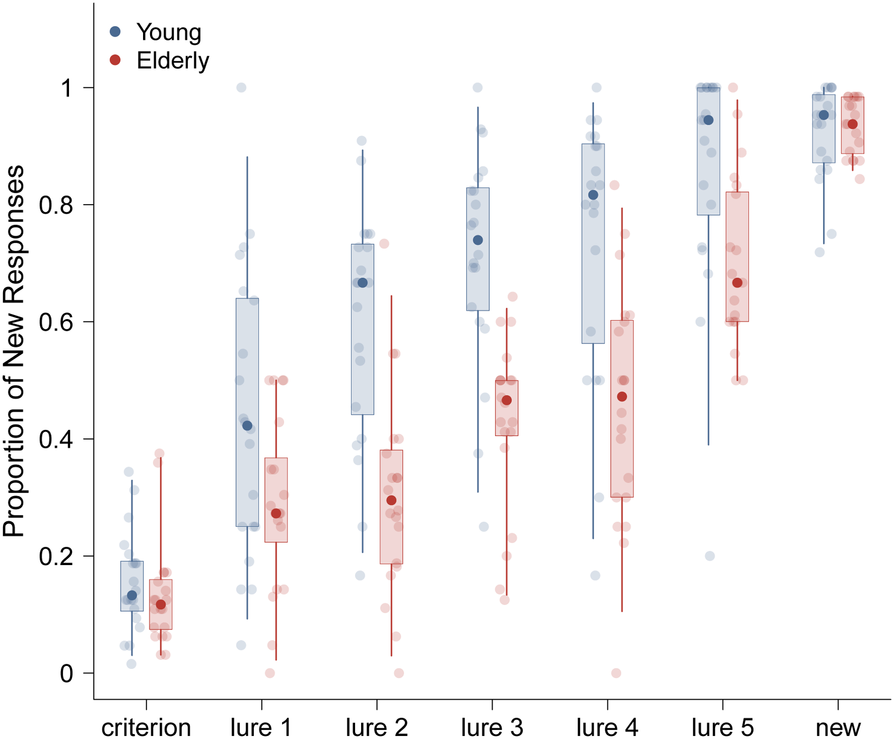
Summary of the MST recognition behavior for young and elderly participants in the Stark et al. (2015) MST task. Box-and-whisker representations of the distribution of the proportion of “new” responses for each stimulus type, for both young and elderly participants, aggregated over all trials.

Cognitive Model

Adaptive design optimization requires a cognitive model. Signal detection theory (SDT: Green & Swets, 1966; MacMillan & Creelman, 2004) provides a widely-used and successful framework for modeling people’s performance on recognition memory tasks (Lockhart & Murdock, 1970). The key assumption is that, when a test stimulus is presented, the output of various memory processes can be summarized in terms of a single measure of recognition strength. People then make an “old” or “new” decision depending on whether the recognition strength is greater or lesser than some criterion.

We use an extended two-response classification form of the SDT model of recognition memory (MacMillan & Creelman, 2004, Ch. 5), adapted to the MST with five levels of lures. This model is shown in Figure 2. It uses the unusual convention of treating the old stimuli as the noise distribution centered at zero and the new stimuli as signals with various levels of novelty, starting with the most similar lure 1 and ranging up to completely new stimuli. While atypical, this can be thought of as detecting a “novelty” signal, rather than detecting a “successfully retrieved” signal. Novelty detection is a well-known construct in the neuroscience of memory (e.g., Brown & Aggleton, 2001) and framing the problem in this manner has advantages for our model. Our framing means that mental samples from the stimulus distribution that are greater than the decision criterion k correspond to “new” responses, and generate either correct rejections or misses, depending on whether the stimulus is really new or old. Similarly, mental samples that fall below the criterion generate “old” responses that are either false alarms or hits.

Figure 2.

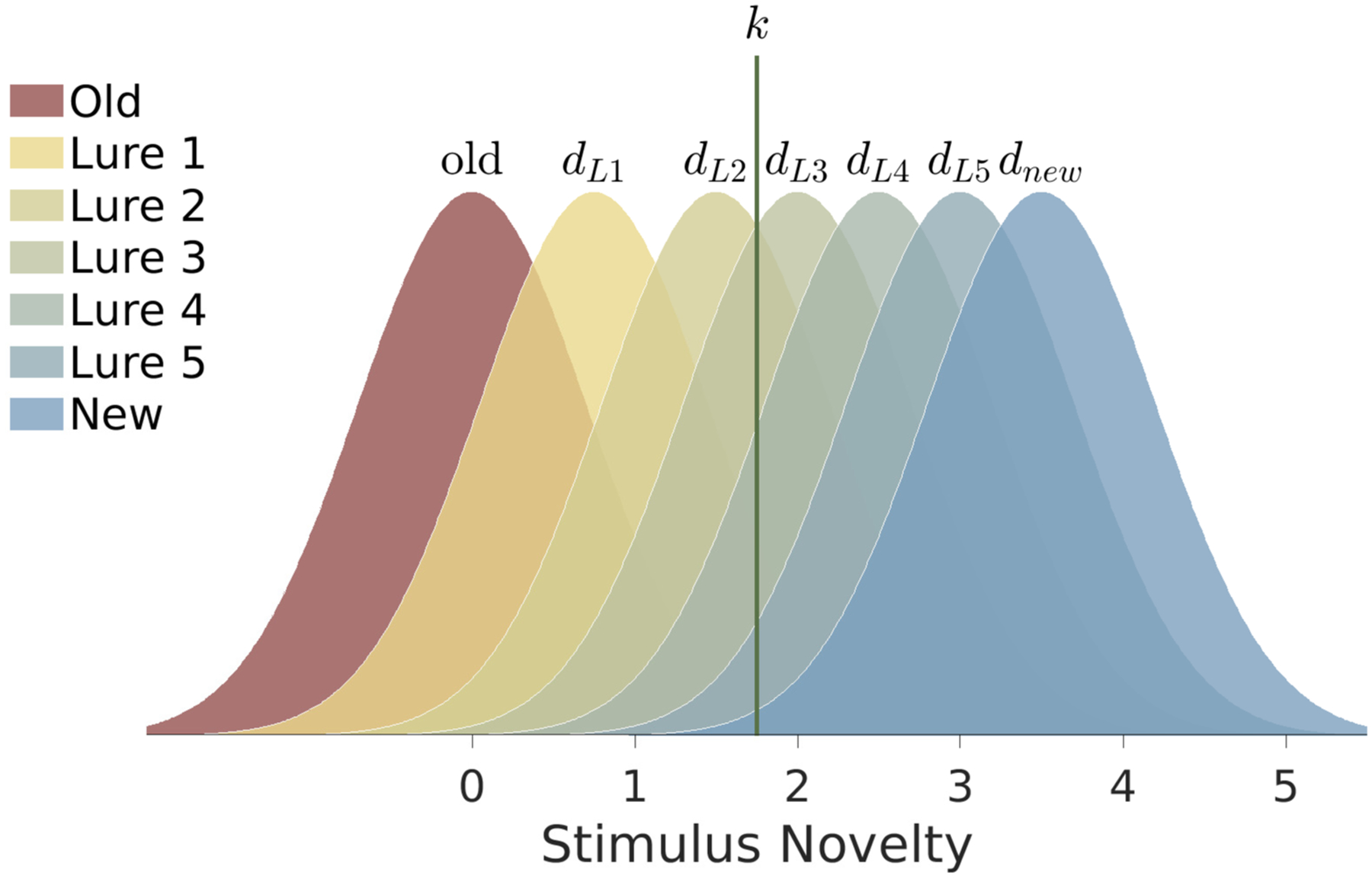
A signal detection theory cognitive model of recognition memory for the MST. Each distribution corresponds to a stimulus type, from which mental samples for specific stimuli are drawn on a trial. If the sample is above the criterion k a “new” response is generated, otherwise an “old” response is generated.

We implement this SDT model as a Bayesian graphical model in JAGS Plummer (2003). JAGS code for the model is available in the supplementary information. Throughout this article, we apply the model using 4 chains with 5000 burnin and 10, 000 posterior samples. The graphical model is shown in Figure 3. Beyond the core SDT assumptions, we use a latent-mixture approach to allow for a low base-rate of responses that correspond to guessing or inattentive decision making (Lee, 2018; Zeigenfuse & Lee, 2010).

Figure 3.

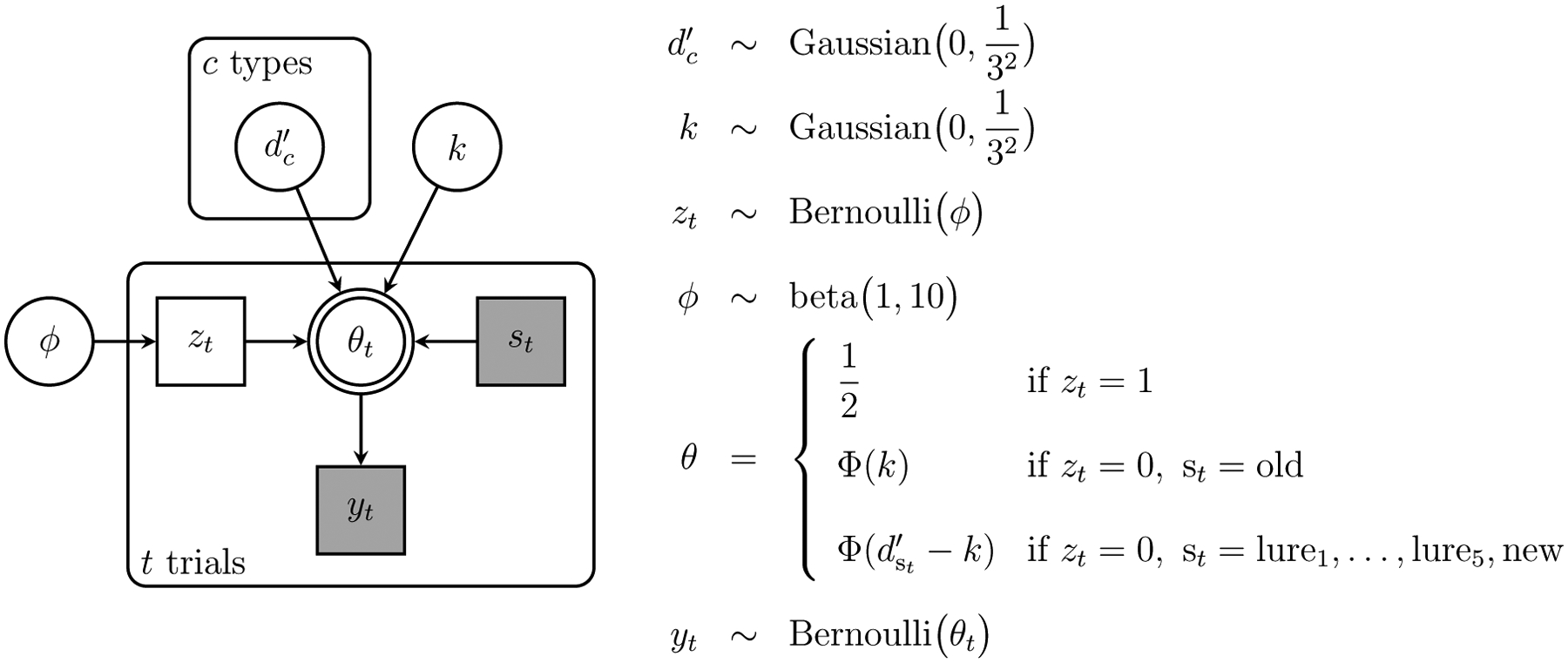
Graphical model representation of the signal detection theory cognitive model, including a latent-mixture trial-level contaminant process.

Formally, the behavior of the participant on trial t is y_t = 1 if they responded “new” and y_t = 0 if they responded “old”. This response is modeled as y_t ~ Bernoulli (θ_t), where the probability of a new response θ_t can follow one of three possibilities:

$${\theta }_t=\{\begin{array}{ll}\frac{1}{2}\hfill & \text{if }{z}_t=1\hfill \\ \Phi (k)\hfill & \text{if }{z}_t=0,{\text{s}}_t=\text{ old}\hfill \\ \Phi \left(k-d_{{\text{s}}_{tia}}^{\prime }\right)\hfill & \text{if }{z}_t=0,{\text{s}}_t={\text{ lure }}_1,\dots ,{\text{ lure }}_5,\text{ new}.\hfill \end{array}$$ (1)

where Φ(·) is the cumulative Gaussian function. The ${\theta }_t=\frac{1}{2}$ possibility corresponds to contaminant behavior and is followed if the latent binary indicator parameter z_t = 1. These latent indicators are independent for each trial z_t ~ Bernoulli(ϕ), with a base-rate ϕ that has a prior favoring relatively low probabilities of contamination ϕ ~ beta(1, 10). If the trial is not a contaminant trial, the probability of a “new” response follows SDT according to whether the present stimulus is old or new.

The discriminability the participant has for a stimulus of type c is $d_c^{\prime }$, where c ∈ {old, lure₁, lure₂, lure₃, lure₄, lure₅, new}. These discriminabilities are given order constrained priors, so that

$$d_c^{\prime }~\text{Gaussian}\left(0,\frac{1}{3^2}\right):d_{{\text{lure }}_1}^{\prime }<\dots <d_{{\text{lure }}_5}^{\prime }<d_{\text{new }}^{\prime }.$$ (2)

The decision criterion independently has prior $k~\text{Gaussian}\left(0,\frac{1}{3^2}\right)$. The priors on d′ and k are intended to allow for a plausible range of values on the discriminability scale defined by the unit variances of the target and noise distributions. The assumed standard deviation of 3 in the prior means, for example, that most d′ and k values will be less than 3 (within one standard deviation), values as high as 6 are plausible (within two standard deviations), but values greater than 9 are very unlikely (beyond three standard deviations).

We applied the model to the Stark et al. (2015) behavioral data in order to test its descriptive adequacy, and to examine the assumption of an additional contaminant process. In terms of descriptive adequacy, the mode of the posterior probability of θ_t matched the observed response y_t on an average of 83% of trials for the young participants, and ranged between 77% and 93% agreement for individual participants. The mean agreement for elderly participants was 84% and ranging between 77% and 92% for individual participants. We interpret this as an adequate level of descriptive adequacy.

To evaluate the contaminant process assumptions, we calculated Bayes factors for each participant comparing the basic model without the contaminant process to the extended model with the contaminant process. Because the basic model is nested within the extended model if the base-rate ϕ = 0 (i.e., there are no contaminant trials), these Bayes factors can be estimated using the Savage-Dickey method (Wetzels et al., 2010). A total of 10 young participants have Bayes factors greater than 3 in favor of the contaminant model, 5 have Bayes factors greater than 3 in favor of the basic model, and the other 5 participants have inconclusive Bayes factors. A total of 11 elderly participants have Bayes factors greater than 3 in favor of the contaminant model, 2 have Bayes factors greater than 3 in favor of the basic model, and the other 7 participants have inconclusive Bayes factors. The Bayes factors in favor of the more general contaminant model are generally larger (Morey et al., 2016), often over 10, and ranging as high as 40. The largest Bayes factor in favor of the basic model is about 4. Overall, we interpret these results as meaning that there is justification in terms of descriptive adequacy for including the contaminant process.

Adaptive Design Optimization

The goal of our application of ADO is to choose the next stimulus so that the expected information it provides about an individual’s recognition parameters is maximally informative. The relevant parameters are the discriminabilities for each stimulus type and the decision criterion, which we represent in a consolidated way

$$\psi =\left(d_{{\text{lure }}_1}^{\prime },\dots ,d_{\text{lure }}^{\prime },d_{\text{new }}^{\prime },k\right).$$ (3)

The current posterior distribution for ψ after t trials is p^t = p(ψ | y_1:t). The next stimulus can be chosen from type c, and will result in the future posterior distribution $p^{t+1}=p\left(\psi \mid y_{1:t},{\widehat{y}}_{t+1}^c\right)$. The $\widehat{y}$ notation makes clear that this last choice is not part of the observed behavioral data, but is being considered as a possible behavior in response to a stimulus of type c being presented on trial t + 1. If the participant were to decide “new” for trial t + 1 then the updated posterior distribution would be $p^{t+1,n}=p\left(\psi \mid y_{1:t},{\widehat{y}}_{t+1}^c=1\right)$. Alternatively, if the participant were to decide old, the updated posterior distribution would be $p^{t+1,o}=p\left(\psi \mid y_{1:t},{\widehat{y}}_{t+1}^c=0\right)$.

We measure the information gained from the additional behavioral data on trial t + 1 using Kullback-Leibler divergence. This is an information theoretic measure of the difference between two distributions and is well suited to our research goals. ADO often uses mutual information or Bayes factors as the key component in a utility function, because the goal is to choose the stimuli that are the most likely to discriminate between two or more competing cognitive models of behavior. Bayes factors provide a measure of how much evidence data provide for one model over another, and so helps choose stimuli that distinguish the models. Mutual information provides a way to measure model mimickry, and so helps choose stimuli that provide a “critical experiment” for which the models make different predictions. In contrast, we rely on the signal detection theory model and aim to infer the discriminability and criterion parameters as quickly as possible. Kullback-Leibler divergence provides a direct and principled measure of the change in the joint posterior distribution of these parameters from trial to trial. In this way, our approach follows that previously developed by Lesmes et al. (2015) for the same purpose.

Formally, if the participant responded “new”, the measured change in information from trial t to t + 1 would be $D_{\text{KL}}\left(p^{t+1,n}\parallel p^t\right)$ and if the participant responded “old” it would be $D_{\text{KL}}\left(p^{t+1,o}\parallel p^t\right)$. The model predicts the probability of an “new” versus “old” response for the stimulus on trial t + 1 by marginalizing over the parameters ψ. This means that the probability of a “new” response is

$$\pi =p\left({\widehat{y}}_{t+1}^c=1\mid y_{1:t}\right)={\int }_{\psi }p\left({\widehat{y}}_{t+1}^c=1\mid \psi \right)p\left(\psi \mid y_{1:t}\right)\text{d}\psi .$$ (4)

The expected information gain from presenting a stimulus of type c is the weighted sum of the “new” and “old” possibilities:

$$\mathbb{E}\left\{D_{\text{KL}}\left(p^{t+1}\parallel p^t\right)\right\}=\pi D_{\text{KL}}\left(p^{t+1,n}\parallel p^t\right)+(1-\pi )D_{\text{KL}}\left(p^{t+1,o}\parallel p^t\right).$$ (5)

The final step is to maximize over c ∈ {old, lure₁, …, lure₅, new} to determine which stimulus should be chosen as

$$\underset{c}{\text{argmax}}\mathbb{E}\left\{D_{\text{KL}}\left(p^{t+1}\parallel p^t\right)\right\}.$$ (6)

Throughout our implementation, we approximate Kullback-Leibler divergence by assuming the joint posterior distribution of ψ is multivariate Gaussian, which gives a closed form for the n = 7 parameters of

$$D_{\text{KL}}=\frac{1}{2}\left\{\text{tr}\left({\Sigma }_{t+1}^{-1}{\Sigma }_t\right)+{\left({\psi }_{t+1}-{\psi }_t\right)}^{\text{T}}{\Sigma }_{t+1}^{-1}\left({\psi }_{t+1}-{\psi }_t\right)-n+\text{ln}\frac{\left|{\Sigma }_{t+1}\right|}{\left|{\Sigma }_t\right|}\right\}.$$ (7)

In applying this approximation, we use posterior expectations for both the mean ψ and for the covariances between discriminabilities in Σ, but assume no covariance between the criterion and the discriminabilities. One limitation of the approximation is that it does not incorporate the truncation that follows from the order constraints on the discriminabilities. These order constraints are only incorporated in the inference that produces the expectations and covariances, In general, however, as more trials are observed, the order constraints have less impact on the inferred joint posterior, because the data themselves provide information that orders and separates the discriminabilities for the different stimulus types.

Evaluation of ADO Method Using Behavioral Data

We evaluate the ADO method on the Stark et al. (2015) experimental data by having ADO reorder the 192 trials that each participant completed. ADO was used to generate a hypothetical order in which the participant would have encountered those trials if it had been applied in their experimental setting. Note that this approach means that the final inferences about ψ using ADO will be the same as those for the original experimental order, because both in the end will have seen the same 192 responses on the same 192 trials. Our evaluation focuses on whether the order that ADO generates results in more quickly making inferences that are close to those that will eventually be made once all of the data have been incorporated.

To assess the performance of the ADO order, we again use Kullback-Leibler divergence, but now to measure the difference between the final posterior distribution ψ* and the posterior after the trial t as $D_{\text{KL}}\left({\psi }_t^{\text{ado}}\parallel {\psi }^{\ast }\right)$. This can be compared to the experiment order $D_{\text{KL}}\left({\psi }_t^{\text{exp}}\parallel {\psi }^{\ast }\right)$.

Individual-Level Results

Figure 4 summarizes the comparative performance of the ADO method for a single participant from the young group. The first seven panels show the change in the marginal posterior distributions for the criterion and the discriminabilities for the lure and new stimulus types. The 95% credible interval of the marginal posterior for each parameter under the actual experimental ordering of stimuli is shown by the shaded yellow region. The 95% credible interval for the hypothetical ADO ordering is shown by the blue lines. The bottom-right panel shows the change in overall Kullback-Leibler divergence for both orderings. The broken line shows the first trial at which ADO was not able to use a stimulus from the highest-ranked type.

Figure 4.

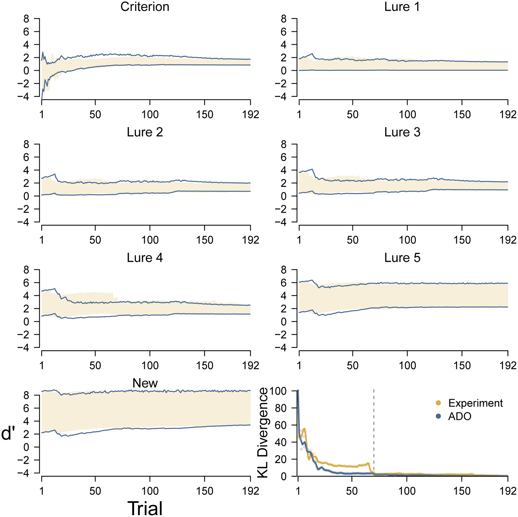
Change in posterior distributions for the discriminability and criterion of the cognitive model over trials, for both the original experimental and hypothetical ADO ordering of trials, for a young participant. The yellow shading and blue lines represent the 95% credible intervals of the marginal posterior distributions for the experimental and ADO orderings, respectively. The bottom-right panel shows the change in overall Kullback-Leibler divergence for both orderings. The broken line shows the first trial at which ADO was not able to use a stimulus from the highest-ranked type.

The bottom right panel shows that the ADO order more quickly leads to a posterior distribution that is close to the final one, especially from about trials 20 to 50. Looking at the individual parameters, it is clear that quicker inference about the discriminability of lure 4 stimuli is the main cause of this improvement. During trials 20 to 50, the ADO ordering leads to a much better inference about the discriminability of these stimuli.

Figure 5 summarizes, in the same way, the comparative performance of the ADO method for a single participant from the elderly group. Once again, the bottom-right panel shows that the ADO order more quickly leads to the final posterior distribution. This advantage is evident after a few trials and is maintained until about 60 trials have been completed, which is well after the point at which the ADO method was no longer always able to use its highest-ranked option. For this elderly participant, it seems clear that better early inferences about lure 5 stimuli is the main reason for the improved ADO performance.

Figure 5.

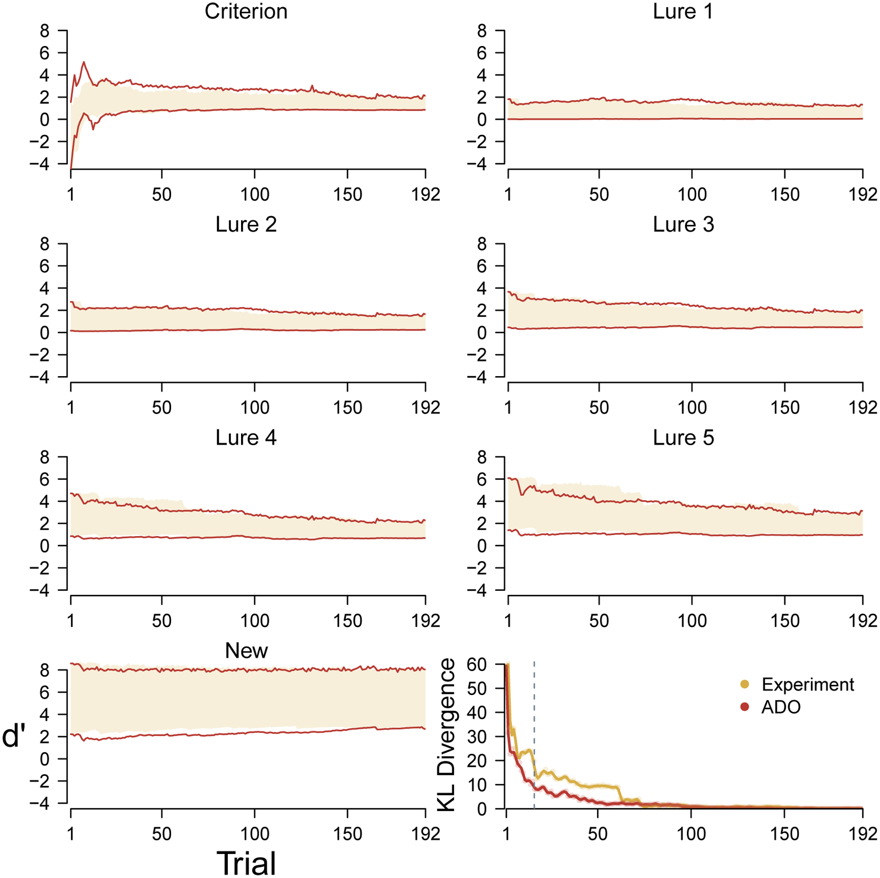
Change in posterior distributions for the discriminability and criterion of the cognitive model over trials, for both the original experimental and hypothetical ADO ordering of trials, for an elderly participant. The yellow shading and blue lines represent the 95% credible intervals of the marginal posterior distributions for the experimental and ADO orderings, respectively. The bottom-right panel shows the change in overall Kullback-Leibler divergence for both orderings. The broken line shows the first trial at which ADO was not able to use a stimulus from the highest-ranked type.

Overall Performance

The results in Figures 4 and 5 are representative of those found for all participants. The results for all participants are provided in the supplementary information and show that ADO usually outperforms the experimental order, especially early in the trial sequence. Sometimes the improvement is large, often it is of the magnitude shown by the two highlighted participants, and there are one or two exceptions.

Figure 6 shows a summary of the performance for young and elderly participants, in terms of the overall Kullback-Leibler measure. In both panels, the shaded yellow regions show the interquartile range for the experimental order and the solid yellow line shows the median across all participants in the group. In the left panel, the shaded blue region and solid blue line show the interquartile range and median for the ADO order applied to young participants. In the right panel, the shaded red region and solid red line show the interquartile range and median for the ADO order applied to elderly participants. For both groups of participants, the results show an overall improvement resulting from the ADO ordering of the trials.

Figure 6.

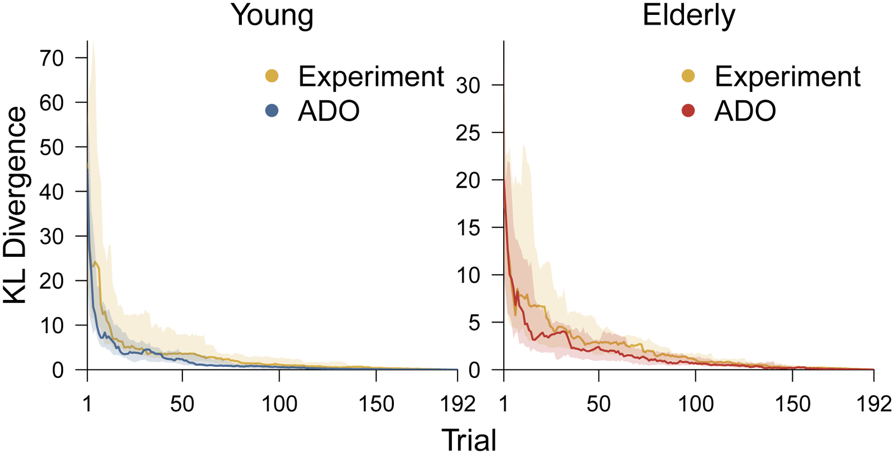
The distribution of change in KL divergence over trials for the ADO and experimental orders. The left panel corresponds to young participants and the right panel corresponds to elderly participants. Within each panel the blue (for young) and red (for elderly) shaded region shows the interquartile range of KL divergence across all participants, and the solid blue and red lines show the median. In both panels, the shaded yellow region shows the interquartile range of KL divergence for the experimental order and the solid line shows the median.

Figure 7 provides another way of comparing the performance of the ADO method to the original experimental order. It summarizes the distribution of the number of trials each method needs to reduce the KL divergence measure to 50%, 55%, …, 95% of its final value, when all of the trials are incorporated in parameter inference. Circular markers show the mean number of trials and error bars show interquartile intervals. The ADO method consistently performs slightly better in reducing KL divergence to about 80% of its final value for both young and elderly participants. It performs much better in achieving the remaining reduction after about 80%. Figure 7 also has the advantage of allowing interpretable statements to understand ADO performance in absolute terms. For example, the ADO ordering reduces the original KL diverge to 90% of its final value on average in about ?? [15ish] trials. This compares to about ?? (45ish) being needed using the original experimental orders.

Figure 7.

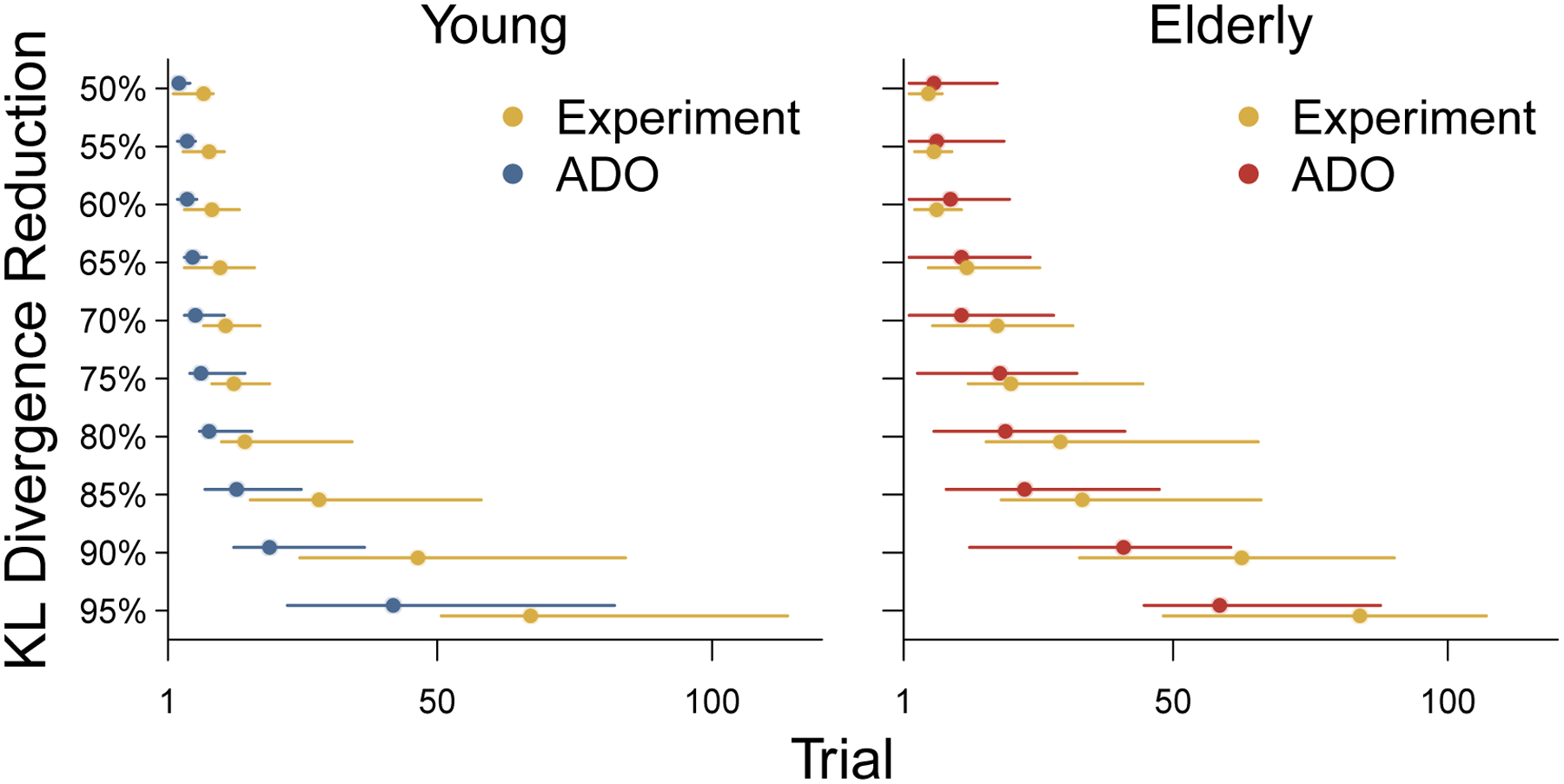
The rate of reduction in KL divergence for both the original experimental and hypothetical ADO ordering of trials for young and elderly participants. Circular markers show the mean number of trials across participants needed to achieve 50%, 55%, …, 95% reduction in KL divergence towards its final value when all trials are incorporated. Error bars show interquartile intervals of the distribution of the number of trials needed.

The Importance of Contaminant Modeling

Most previous applications of ADO in cognitive science do not incorporate contaminant processes in the cognitive models being used or compared. The one exception is provided by Lesmes et al. (2015), who assumed a fixed proportion of two percent of trials are lapse errors. Their modeling does not identify which individual trials involved these lapses but simply assumed they were equally likely to be false alarms and misses. Our approach, based on a latent-mixture model that makes inferences about contamination trial by trial, is considerably more detailed, which raises the question of whether it is necessary or useful.

The model infers a non-negligible number of contaminant trials for many participants. The average is 5.9 trials for young participants, ranging from 0 to 26 trials at the individual level, and 9.5 for elderly participants, ranging from 1 to 23 trials at the individual level. If the contaminant process is removed, and these trials are not identified, ADO produces orders that generally do not improve upon the experimental order. This is not a fault in the logic of ADO, but rather an inadequacy in how the discriminability and criterion parameters are measured by the cognitive model. Figure 8 shows a concrete example of this different assessment for the elderly participant considered in Figure 5. The results in Figure 8 show the inferences about the discriminabilities and decision criterion, and the overall KL divergence, using the same cognitive model but without the contaminant process.

Figure 8.

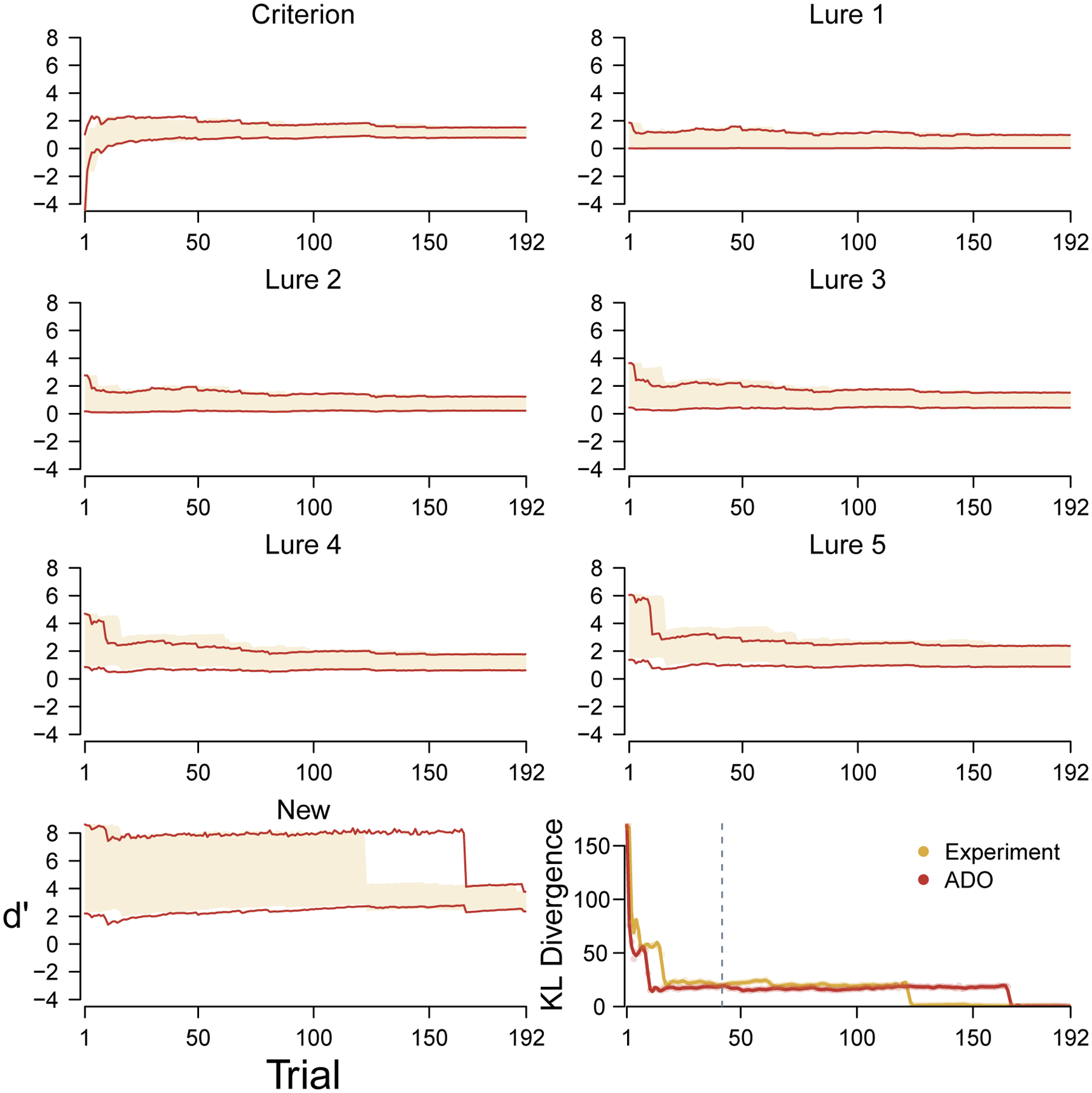
Analysis of both the original experimental and hypothetical ADO ordering of trials based on a version of the cognitive model that does not include a contaminant, for the same elderly participant as Figure 5.

Through the first 170 or so trials in the ADO order, this elderly participant has been observed to be as accurate in responding to new stimuli. This leads the ADO method to infer a large discriminability and to expect their future responses also to be correct. This expectation, in turn, gives the presentation of new stimuli a low priority in terms of expected information. The participant, however, has a single contaminant response to a new stimulus—a momentary lapse during which the participant decides “old”—that proves to be extremely surprising. It causes a large decrease in the inferred discriminability for new stimuli when it is encountered around trial 170. According to the KL measure by which the ADO ordering is assessed, this sudden change appears meaningful, and the ADO order is judged to have performed poorly for not prioritizing a stimulus type that led to this important update.

Figure 8 does not represent an isolated occurrence in our data. This occurs for the majority of both young and elderly participants. For this reason, the ability to identify specific contaminant trials in a principled way is an important part of the good performance of the ADO method. An interesting follow-up question is whether allowing for contaminant responses would continue to be important if the ADO approach was able to reduce the MST to a small number of trials. It might be that contaminant behavior mostly occurs on later trials as the participant loses attention or motivation. Our results suggest that this is not the case. On average, 22% of the contaminant trials inferred for young participants occur within the first 64 trials (i.e., the first third of the task). For elderly participants, the average is 41%, which means that contaminant behavior occurs disproportionately early.

Stimulus Selection

One way to understand the performance of ADO is to look at the sequence of stimuli it chooses, in terms of the stimulus types. Figure 9 shows this information for the same young participant considered in Figure 4. Each panel corresponds to a different stimulus type. The lines show the cumulative distribution of the trials at which stimuli of that type were presented, with blue lines corresponding to the ADO order, and yellow lines corresponding to the experimental order. The circles on the ADO indicate that the presented stimulus was the one with the greatest expected information gain.

Figure 9.

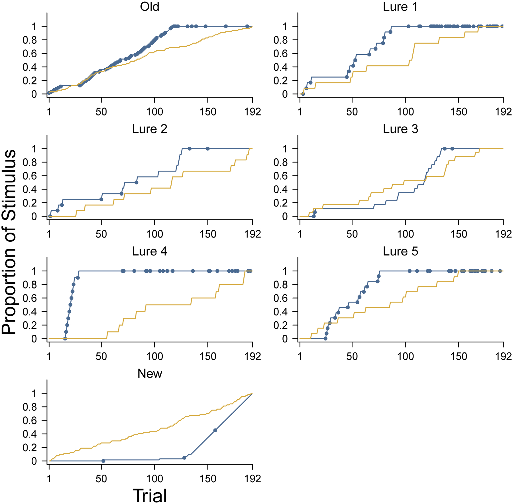
Order in which stimulus types are presented by ADO for a young participant. The panels correspond to the different stimulus types. Blue lines show the proportion of stimuli of that type that have been presented after each trial by ADO. Blue circular markers on the line indicate that the stimulus type was the one with maximum expected information gain according to ADO. Yellow lines show the proportion of stimuli of that type after each trial in the experimental order.

As a concrete example, consider the panel for lure 4 stimuli. Under ADO, the first lure 4 stimulus was presented after about 10 trials, and this started a sequence of presenting nine more lure 4 stimuli in the next 10 trials. At this point, all of the available lure 4 stimuli had been presented. Later in the experiment, however, starting around trial 65, the ADO method found lure 4 stimuli again to be the highest priority. Similar patterns are seen for lure 1 and lure 5 stimuli, which ADO prioritized and exhausted relatively early in the experiment. New stimuli, in contrast, are rarely the first priority for ADO, and are mostly presented in the final trials, when they are the only remaining stimuli.

Recall that the improved performance of ADO for this participant, as shown in the analysis in Figure 4 largely resulted from improved inference about the discriminability of lure 4 stimuli. It is clear from Figure 9 how ADO achieves this. It also seems likely based on Figure 9 that ADO performance would be improved further if more lure 4 stimuli, and perhaps also lure 1 and lure 5 stimuli, had been available. These stimuli could replace the new stimuli. Intuitively, this young participant had no difficulty identifying new stimuli and so there was no need to continue to test their abilities. Those trials would have been better focused measuring in a more fine-grained way their ability to discriminate the lures.

This set of stimulus order findings for a single participant is highly representative of what is found across all participants in both age groups. The stimulus order analysis for every participant is provided in the supplementary information, but Figure 10 provides a summary. It shows the average proportion of each stimulus type used after every trial for both the young and elderly participant groups. It is clear that, for both groups, the new stimuli are generally given the lowest priority, and old stimuli are also presented after lure stimuli. It is interesting to note that lure 5 stimuli are generally presented the earliest for elderly participants, but lures that are more similar to studied stimuli are emphasized for young participants. This pattern is consistent with how challenging highly similar lures are for older participants and how easy very different lures are for younger participants.

Figure 10.

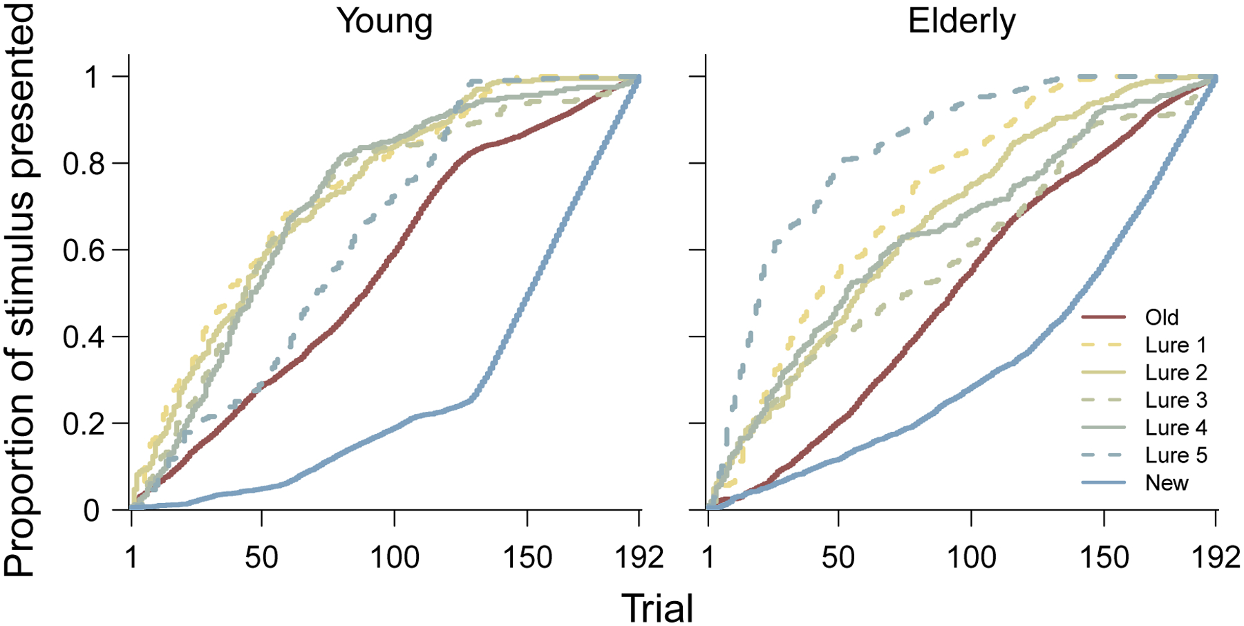
Average proportion of each stimulus type are presented by ADO after each trial, aggregated over all young participants (left panel) and all elderly participants (right panel).

Overall, our results suggest that, for most participants, having one-third of the trials present new stimuli is inefficient, because they are rarely the most likely to provide the most information. For many participants, having one-third old stimuli is also too many. The ADO order usually focuses quickly on lure stimuli that are at the inflection points between stimulus similarity and discriminability. These are the important stimuli to measure well to understand how people’s memory performs across the range of stimuli considered in the MST.

A Simulated Evaluation for the MST Without Stimulus Restrictions

To explore how ADO could improve inferences if it was not restricted in the available stimuli, we conducted a simulation study. We used the three young and three elderly participants with 25th, 50th, and 75th percentile accuracy within their group to represent low-, average-, and high-accuracy individuals. We then simulated the testing phase of the MST using the posterior distributions of these participants to generate behavioral data. The simplest approach would have been to use the posterior means as fixed values to generate the behavior of each simulated participant. While using single “ground truth” values in simulation studies is common practice in cognitive modeling, it can be argued to be unrealistic. Real participants almost certainly fluctuate over 192 trials in their ability to discriminate and recognize stimuli and their decision strategies. Assuming fixed parameters thus generates behavior that lacks real-world variability, especially given that the SDT model is a simplified approximation to the cognitive processes used. Accordingly, we chose to use a distribution of values as the ground truth for each participant.

Specifically, we created Gaussian distributions for the discriminabilities and criterion of each participant and, on each trial, sampled specific d′ and k values from these distributions to generate an “old” or “new” response to the presented stimulus according to the model. The Gaussian distributions were defined by the inferred posterior mean of the participant and the inferred standard deviation of the participant’s observed behavioral data, but with the standard deviation reduced. The motivation for reducing the standard deviation was that the ground truth distribution conceptually represents the “true” underlying distribution for the participant. The inference from the MST task is based on a limited number of trials and so has uncertainty beyond the inherent variability in the true memory discriminabilities and decision criteria used by the participant. Reducing the variance of the parameters used to simulate data is intended to remove this uncertainty. We chose to reduce the standard deviations by a factor of four. There is nothing principled about this choice, but it seems like a reasonable approximation. The key outcome is that simulated participant behavior is based on their inferred d′ and k, but maintains a realistic level of variability.

Figure 11 summarizes the results of the simulation study. Each panel corresponds to a participant, with the top and bottom rows showing young and elderly participants respectively, and left, middle, and right panels showing low-, average-, and high-accuracy participants within their age group. Within each panel the blue (young) and red (elderly) line shows the median change in KL divergence using the ADO method, with shading showing the interquartile interval. The yellow lines show the median change in KL divergence for a set of randomly chosen experimental orders among those used in the Stark et al. (2015) experiment, with shading again showing interquartile intervals.

Figure 11.

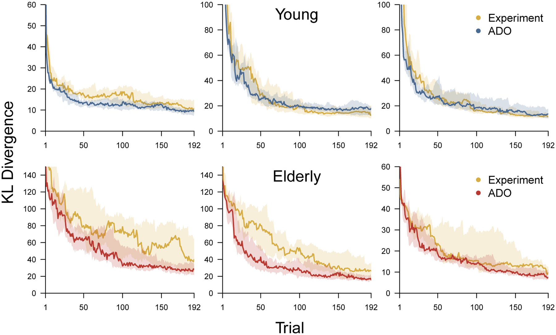
The distribution of change in KL divergence over trials for the ADO and experimental orders for six simulated participants in an MST experiment that allows for unlimited stimuli of each type. The top panels correspond to young participants and the bottom panels correspond to elderly participants. In each row, the leftmost panel represents a low-accuracy participant from that group, the middle panel represents an average-accuracy participant, and the right panel represents a high-accuracy participant. Within each panel the blue (for young) and red (for elderly) shaded region shows the interquartile range of KL divergence across all participants, and the solid blue and red lines show the median. In both panels, the shaded yellow region shows the interquartile range of KL divergence for a collections of experimental orders and the solid line shows the median.

Figure 11 shows that the ADO order generally outperforms random experimental orders. The ADO order is better on average for the first 50 or so trials in all cases, and maintains its advantage for the low-performing young and elderly simulated participant, and the average-performing elderly participant. The maintained advantage seems likely to be the result of having stimuli of every type available on every trial. The interquartile ranges show that the worst case performance of experimental orders is much worse for elderly participants.

A second analysis provided by the simulation study is shown in Figure 12. It shows the frequency with which each type of stimulus was used by the ADO method for the three young and three elderly participants, and compares those frequencies to those used in the experimental order. It is clear that ADO uses far fewer than the 64 new test stimuli used by the MST design. Young participants, in particular, were almost never presented with new stimuli, presumably because it is clear from their performance on easy lures that they will respond correctly. The distributions of stimuli for young and elderly participants would provide a very simple way potentially to improve the MST design, not by the adaptive presentation of stimuli, but just by changing the numbers of each type presented.

Figure 12.

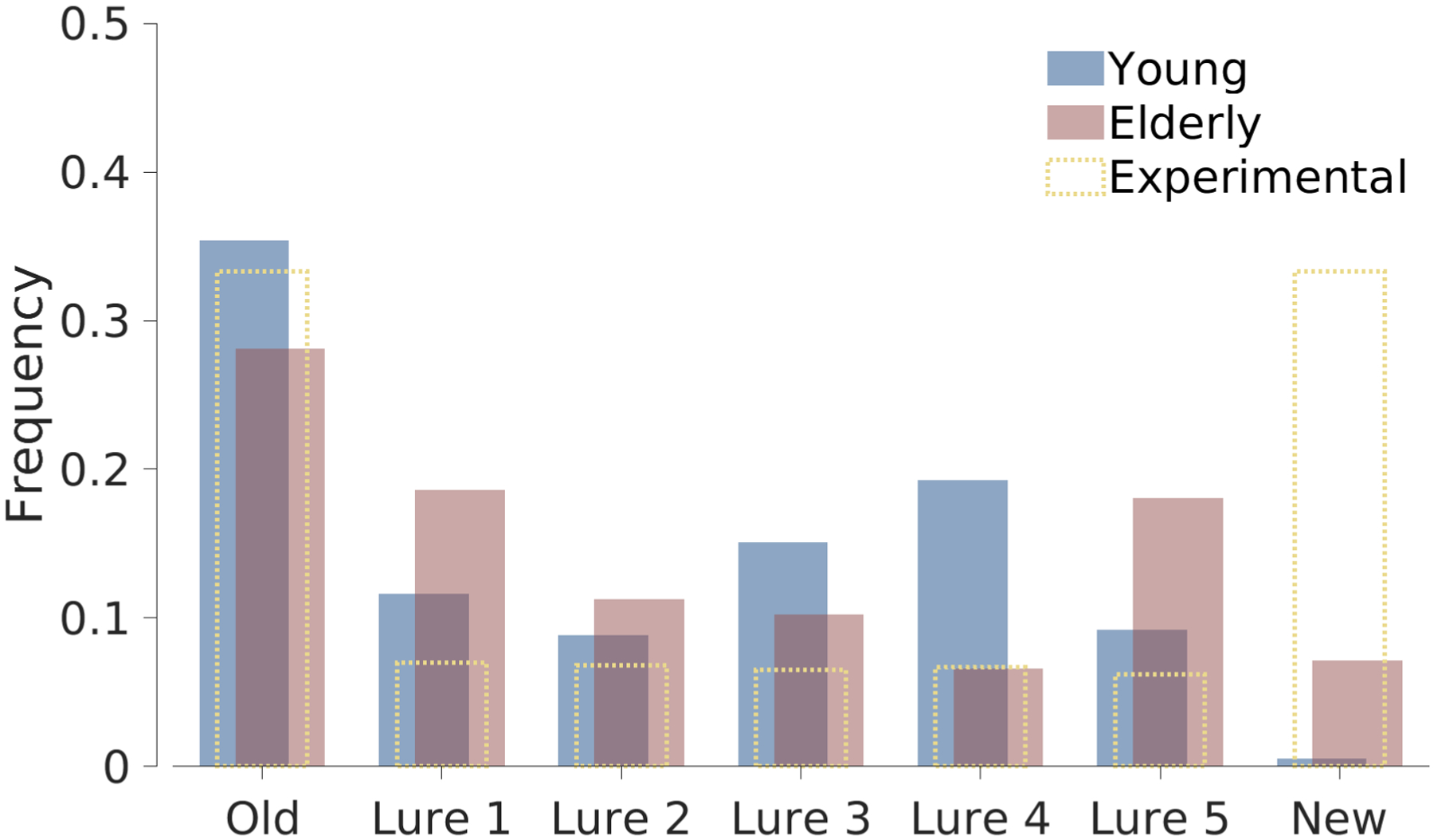
Frequency of presentation of each stimulus type for simulated young and simulated elderly participants, and the original experimental design of the MST.

Discussion

Recognition memory is a foundational phenomenon that is widely studied in cognitive science, and the MST is an important measurement task that is used in clinical and neuropsychological settings. Our ADO method generally improves how quickly inferences about the memory discriminabilities and decision criterion measured by the MST are made for individual participants. The focus of our scientific goals on measurement rather than model comparison is different from many previous ADO applications in cognitive science. The specific statistical approach we developed follows most closely previous work by Lesmes et al. (2015), and provides another useful worked example for measurement-focused applications.

Improving the Cognitive Model

While our results are promising, they are only a first step in applying ADO to the MST. There are two main ways toward improving performance. The first way is through improving the cognitive model. It is generally the case that the better the underlying cognitive model, the better ADO will perform, because the parameters being measured will be better characterized, and because the predictions about future behavior will be better. The inclusion of a contaminant process in our model is a good example of the need for appropriate cognitive models. A very promising direction for further model improvement is using hierarchical extensions to model individual differences with groups (Rouder & Lu, 2005). In the Stark et al. (2015) data, there are clear group differences between the young and elderly, with individual differences within the groups. Accounting for this structure with a hierarchical model should lead to quicker and more confident inferences about the parameters of individuals, and improve the performance of ADO (Gu et al., 2016; Kim et al., 2014).

More ambitious model development should focus on the sequential nature of the MST test phase. It seems unlikely that people treat each trial as a completely separate cognitive decision, but that is what our current model assumes. A better model would incorporate some sort of learning capability and allow for the possibility of sequential effects. This may be especially important if the sequence of stimuli that ADO presents impacts participants’ recognition memory behavior. For example, if ADO leads to the consecutive presentation of many difficult lure 1 stimuli, that may impact the concentration or motivation of a participant. One way to safeguard against these effects would be to place constraints on how ADO orders stimuli. A better way would be to maintain the current unconstrained model-based approach, but use a model that can predict the sequential effects of difficult stimuli, so that they are automatically factored into the ADO optimization. A related problem is allowing for changes in strategy or other non-stationarities in cognitive performance. Hou et al. (2016) present a worked example of extending ADO to this setting, using discriminative statistical methods to infer changes in contrast sensitivity functions for a visual task. An alternative, but very challenging, approach would be to extend the generative cognitive modeling approach to allow for switching strategies (Bröder & Schiffer, 2006; Lee & Gluck, 2021; Lee et al., 2015; Rieskamp & Otto, 2006).

Finally, it would also be worth exploring alternatives to SDT as the cognitive modeling framework. SDT is a well-established and successful model of recognition memory and our extension to MST by adding order-constrained lure distributions is a natural one. But the descriptive adequacy of our SDT model is far from perfect and it may be that alternative assumptions, or an entirely different modeling approach, accounts for people’s behavior better. One alternative approach is provided by multinomial processing trees, which are also often used to model recognition memory (Batchelder & Riefer, 1980; Erdfelder et al., 2009).

Extensions to ADO

The second way to improve current performance is to improve or extend ADO itself. Our approach relies on greedy optimization, because it chooses only the stimulus for the next trial. There is some work in ADO considering optimization that looks further ahead by using dynamic programming methods Kim et al. (2017). It is currently an open question as to whether the significant additional computational effort required leads to an equally significant improvement in performance. It is, however, a logical extension of the current greedy optimization and is worth considering.

It may also be worth thinking about whether expected information gain is always the right measure to optimize over. It could be that alternative measures, such as maximizing the worst case information gain–intuitively, minimizing the possibility that nothing is learned from the next trial—is more robust or effective than maximizing the average. Alternatively, Ahn et al. (2020) present a case study of ADO optimizing delay discounting experiments in terms of test-retest reliability measures. That criterion is also a natural one for the clinical settings in which MST is used. Ultimately, the choice of criterion depends on exactly what the goals of the experiment are, and this will vary in terms of the practical research context. For example, in a clinical setting in which a patient may only be able to perform for some small but unknown number of trials, guaranteeing that at least some information is gained about their recognition memory from the trials they do complete in every session may be more useful than maximizing what is expected to be learned. One way to think about this trade-off is in terms of average information gain versus the variance in information gain.

Applying ADO to the MST

The obvious next step is to test ADO in MST experiments where there are not any limits on the availability of each stimulus. Our simulation study results show promising performance, but rely on data generated by a cognitive model that roughly approximates the processes people really use to make decisions. Our current implementation relies on inferring the full joint posterior distribution of the cognitive model at each trial. This involves Markov-chain Monte Carlo sampling implemented by JAGS, and is probably too slow to work in real time. It should be possible to develop point estimate approximations that can be quickly computed, and the current full implementation would then serve as a benchmark to test the performance of the approximation.

Finally, we are interested in extending ADO methods to other forms of the MST. One variant of the MST allows participants to make “similar”, as well as “old” and “new” responses. There is evidence that assuming a uni-dimensional representation consistent with SDT, in which the “similar” response corresponds to mental samples between “old” and “new” may not be reasonable (Lacy et al., 2011). Thus some other sort of cognitive model may be needed, perhaps in the form of a multidimensional signal detection theory model. Once again, multinomial processing trees provide a plausible alternative approach.

Another variant of the MST is a continuous version of the task that presents sequences of stimuli and asks participants whether the current stimulus has been studied as part of this sequence before. This variant is appealing in terms of clinical application, because it does not need time-consuming training trials. Applying ADO to this MST task seems likely to require an extended cognitive model with a more detailed account of learning and memory than our SDT model provides. In particular assumptions would be needed about how the memory strength for encountered stimuli changes according to the number of trials before it is presented as a test stimulus (Shepard & Teghtsoonian, 1961).

Regardless of these extensions, our results have several important insights that can already be used to improve the use of the MST in research. First, it is clear that shorter tests are quite viable and that the amount of information gained in the last half of the test phase is quite small. This is consistent with empirical reports showing that half-length versions of the test were still reliable (Stark et al., 2015). Secondly, it is clear that the choice of the level of lure similarity used in testing should be viewed as a parameter that can be optimized. For example, while removing all new stimuli from the test session would likely be impractical from a behavioral standpoint, our results suggest that their measurement value is quite low and that the more dissimilar lures, such as lure 4 and lure 5, are far more informative.

Conclusion

The MST is an important task for measuring recognition memory, especially in clinical settings. We have developed a model-based approach for improving the efficiency of one common version of the task using ADO methods to choose which stimulus is presented on each test trial depending on the previous behavior of the person being tested. Analysis of experimental data and a simulation study suggest that our method is a promising first step to improving how quickly and efficiently the MST can measure recognition memory.

Appendix

Figure 13 shows the change in KL divergence over trials for all 40 participants from Stark et al. (2015). The top 20 panels correspond to the young participants and the ADO performance is shown in blue. The bottom 20 panels correspond to the elderly participants and the ADO performance is shown in red. The performance of the experimental order is always shown in yellow. The broken line shows the first trial at which ADO was not able to use a stimulus from the highest-ranked type.

Figure 13.

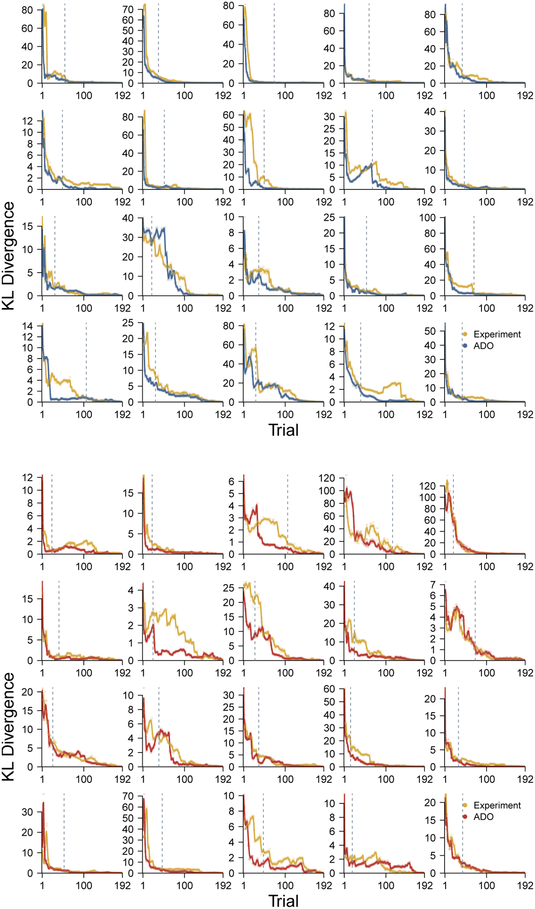
The change in KL divergence for all 40 participants from Stark et al. (2015).

References

- Ahn W-Y, et al. (2020). Rapid, precise, and reliable measurement of delay discounting using a Bayesian learning algorithm. Scientific Reports, 10, 1–10. [DOI] [PMC free article] [PubMed] [Google Scholar]
- Batchelder WH & Riefer DM (1980). Separation of Storage and Retrieval Factors in Free Recall of Clusterable Pairs. Psychological Review, 87, 375–397. [Google Scholar]
- Bröder A & Schiffer S (2006). Stimulus format and working memory in fast and frugal strategy selection. Journal of Behavioral Decision Making, 19, 361–380. [Google Scholar]
- Brown MW & Aggleton JP (2001). Recognition memory: what are the roles of the perirhinal cortex and hippocampus? Nature Reviews Neuroscience, 2, 51–61. [DOI] [PubMed] [Google Scholar]
- Cavagnaro DR, Aranovich GJ, McClure SM, Pitt MA, & Myung JI (2016). On the functional form of temporal discounting: An optimized adaptive test. Journal of Risk and Uncertainty, 52, 233–254. [DOI] [PMC free article] [PubMed] [Google Scholar]
- Cavagnaro DR, Myung JI, Pitt MA, & Kujala JV (2010). Adaptive design optimization: A mutual information-based approach to model discrimination in cognitive science. Neural Computation, 22, 887–905. [DOI] [PubMed] [Google Scholar]
- Cavagnaro DR, Pitt MA, Gonzalez R, & Myung IJ (2013). Discriminating among probability weighting functions with adaptive design optimization. Journal of Risk and Uncertainty, 47, 255–289. [DOI] [PMC free article] [PubMed] [Google Scholar]
- Cavagnaro DR, Pitt MA, & Myung JI (2011). Model discrimination through adaptive experimentation. Psychonomic Bulletin & Review, 18, 204–210. [DOI] [PMC free article] [PubMed] [Google Scholar]
- Erdfelder E, Auer T-S, Hilbig BE, Aßfalg A, Moshagen M, & Nadarevic L (2009). Multinomial processing tree models: A review of the literature. Zeitschrift für Psychologie/Journal of Psychology, 217, 108–124. [Google Scholar]
- Ferguson SA, Hashtroudi S, & Johnson MK (1992). Age differences in using source-relevant cues. Psychology and Aging, 7, 443. [DOI] [PubMed] [Google Scholar]
- Green DM & Swets JA (1966). Signal Detection Theory and Psychophysics. New York: Wiley. [Google Scholar]
- Gu H, Kim W, Hou F, Lesmes LA, Pitt MA, Lu Z-L, & Myung JI (2016). A hierarchical Bayesian approach to adaptive vision testing: A case study with the contrast sensitivity function. Journal of Vision, 16, 1–17. [DOI] [PMC free article] [PubMed] [Google Scholar]
- Hou F, Lesmes LA, Kim W, Gu H, Pitt MA, Myung JI, & Lu Z-L (2016). Evaluating the performance of the quick CSF method in detecting contrast sensitivity function changes. Journal of vision, 16(6), 1–19. [DOI] [PMC free article] [PubMed] [Google Scholar]
- Kim W, Pitt MA, Lu Z-L, & Myung JI (2017). Planning beyond the next trial in adaptive experiments: A dynamic programming approach. Cognitive Science, 41, 2234–2252. [DOI] [PMC free article] [PubMed] [Google Scholar]
- Kim W, Pitt MA, Lu Z-L, Steyvers M, & Myung JI (2014). A hierarchical adaptive approach to optimal experimental design. Neural Computation, 26, 2465–2492. [DOI] [PMC free article] [PubMed] [Google Scholar]
- Koutstaal W, Schacter DL, Galluccio L, & Stofer KA (1999). Reducing gist-based false recognition in older adults: encoding and retrieval manipulations. Psychology and Aging, 14, 220. [DOI] [PubMed] [Google Scholar]
- Lacy JW, Yassa MA, Stark SM, Muftuler LT, & Stark CE (2011). Distinct pattern separation related transfer functions in human CA3/dentate and CA1 revealed using high-resolution fMRI and variable mnemonic similarity. Learning & Memory, 18, 15–18. [DOI] [PMC free article] [PubMed] [Google Scholar]
- Lee MD (2018). Bayesian methods in cognitive modeling. In Wixted J & Wagenmakers E-J (Eds.), The Stevens’ Handbook of Experimental Psychology and Cognitive Neuroscience. Volume 5: Methodology chapter 2, (pp. 37–84). John Wiley & Sons, fourth edition. [Google Scholar]
- Lee MD & Gluck KA (2021). Modeling strategy switches in multi-attribute decision making. Computational Brain & Behavior, 4, 148–163. [Google Scholar]
- Lee MD, Newell BR, & Vandekerckhove J (2015). Modeling the adaptation of the termination of search in human decision making. Decision, 1, 223–251. [Google Scholar]
- Lesmes LA, Lu Z-L, Baek J, Tran N, Dosher BA, & Albright TD (2015). Developing Bayesian adaptive methods for estimating sensitivity thresholds (d′) in Yes-No and forced-choice tasks. Frontiers in Psychology, 6, 1070. [DOI] [PMC free article] [PubMed] [Google Scholar]
- Lockhart RS & Murdock BB (1970). Memory and the theory of signal detection. Psychological Bulletin, 74, 100–109. [Google Scholar]
- MacMillan N & Creelman CD (2004). Detection theory: A user’s guide (2nd ed.). Hillsdale, NJ: Erlbaum. [Google Scholar]
- Morey RD, Wagenmakers E-J, & Rouder JN (2016). Calibrated Bayes factors should not be used: A reply to Hoijtink, van Kooten, and Hulsker. Multivariate Behavioral Research, 51, 11–19. [DOI] [PubMed] [Google Scholar]
- Myung JI, Cavagnaro DR, & Pitt MA (2013). A tutorial on adaptive design optimization. Journal of Mathematical Psychology, 57, 53–67. [DOI] [PMC free article] [PubMed] [Google Scholar]
- Plummer M (2003). JAGS: A program for analysis of Bayesian graphical models using Gibbs sampling. In Hornik K, Leisch F, & Zeileis A (Eds.), Proceedings of the 3rd International Workshop on Distributed Statistical Computing (DSC; 2003). [Google Scholar]
- Rieskamp J & Otto P (2006). SSL: A theory of how people learn to select strategies. Journal of Experimental Psychology: General, 135, 207–236. [DOI] [PubMed] [Google Scholar]
- Rouder JN & Lu J (2005). An Introduction to Bayesian Hierarchical Models with an Application in the Theory of Signal Detection. Psychonomic Bulletin & Review, 12, 573–604. [DOI] [PubMed] [Google Scholar]
- Shepard RN & Teghtsoonian M (1961). Retention of information under conditions approaching a steady state. Journal of Experimental Psychology, 62(3), 302–309. [DOI] [PubMed] [Google Scholar]
- Stark SM, Kirwan CB, & Stark CEL (2019). Mnemonic similarity task: A tool for assessing hippocampal integrity. Trends in Cognitive Sciences, 23, 938–951. [DOI] [PMC free article] [PubMed] [Google Scholar]
- Stark SM, Stevenson R, Wu C, Rutledge S, & Stark CEL (2015). Stability of age-related deficits in the mnemonic similarity task across task variations. Behavioral Neuroscience, 129, 257–268. [DOI] [PMC free article] [PubMed] [Google Scholar]
- Tang Y, Young CJ, Myung JI, Pitt MA, & Opfer JE (2010). Optimal inference and feedback for representational change. In Proceedings of the Annual Meeting of the Cognitive Science Society, volume 32. [Google Scholar]
- Wetzels R, Grasman RPPP, & Wagenmakers E (2010). An encompassing prior generalization of the Savage-Dickey density ratio test. Computational Statistics and Data Analysis, 54, 2094–2102. [Google Scholar]
- Yang J, Pitt MA, Ahn W-Y, & Myung JI (2021). ADOpy: a python package for adaptive design optimization. Behavior Research Methods, 53, 874–897. [DOI] [PMC free article] [PubMed] [Google Scholar]
- Zeigenfuse MD & Lee MD (2010). A general latent assignment approach for modeling psychological contaminants. Journal of Mathematical Psychology, 54, 352–362. [Google Scholar]
- Zhang S & Lee MD (2010). Optimal experimental design for a class of bandit problems. Journal of Mathematical Psychology, 54, 499–508. [Google Scholar]