

Summary
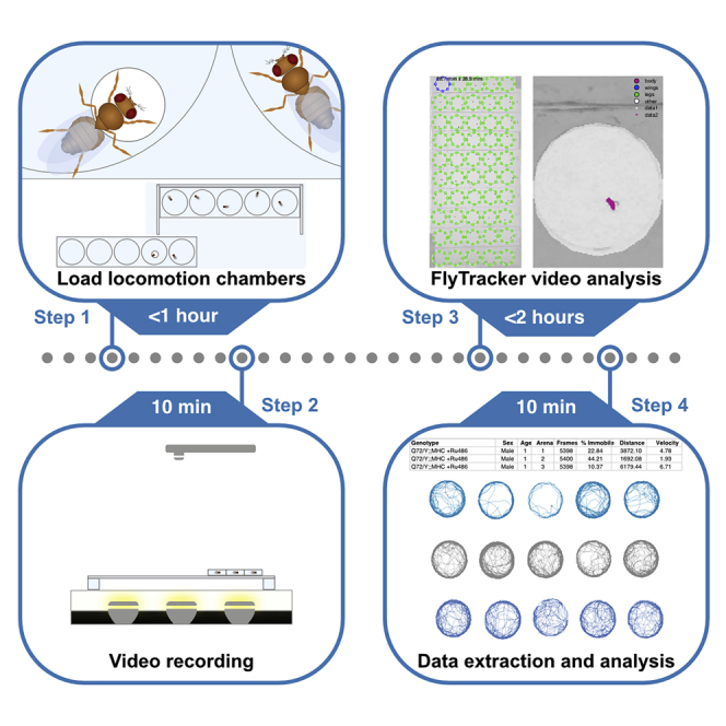
The quantitative analysis of locomotion is used to study many biological processes. Here, we describe how to record the locomotion of up to 50 Drosophila individuals and process the resulting video files using FlyTracker. We detail the use of modifiable MatLab scripts to process structure array files generated by FlyTracker. We have applied this to study Drosophila movement during aging, but it could be used to address a variety of research questions.
For complete details on the use and execution of this protocol, please refer to Barwell et al. (2021).1
Subject areas: Genetics, Model Organisms, Neuroscience, Behavior
Graphical abstract
Highlights
-
•
Detailed and fast protocol for longitudinal studies of spontaneous locomotion
-
•
Optimized protocol to measure variables affected by muscle strength
-
•
Protocol to measure up to 50 individuals simultaneously
Publisher’s note: Undertaking any experimental protocol requires adherence to local institutional guidelines for laboratory safety and ethics.
The quantitative analysis of locomotion is used to study many biological processes. Here, we describe how to record the locomotion of up to 50 Drosophila individuals and process the resulting video files using FlyTracker. We detail the use of modifiable MatLab scripts to process structure array files generated by FlyTracker. We have applied this to study Drosophila movement during aging, but it could be used to address a variety of research questions.
Before you begin
Drosophila media preparation
Timing: 2 days
This step describes the preparation of 10 L of Drosophila food media.
CRITICAL: Do not use tap water. Reverse osmosis (RO) or distilled water must be used.
-
1.
Spray the kettle (or cooking pot) with 80% EtOH and let dry.
-
2.Prepare anti-fungal solution.
-
a.Weigh 18.5 g Methyl-p-Hydroxybenzoic Acid in a 500 mL sealable container.
-
b.Add 184 mL 95% EtOH.
-
c.Seal and swirl several times until it is fully dissolved.
-
a.
-
3.Weigh dry ingredients in a 5 L plastic beaker.
-
a.94.3 g Agar-Agar powder (food-grade is cheaper than laboratory-grade).
-
b.337.7 g active dry Yeast.
-
c.819.7 g dry milled corn (cornmeal).
-
a.
-
4.
Transfer the weighed ingredients to the kettle.
-
5.
Add 2 L water.
-
6.
Mix water and ingredients with a cooking spatula to obtain a smooth paste.
-
7.Prepare molasses solution with reduced viscosity.
-
a.Pour 2 L RO water in the 5 L plastic beaker.
-
b.Add 0.8 L molasses and mix with spatula.
-
a.
-
8.
Add molasses solution to the kettle and mix with spatula.
-
9.
Add 7.5 L water and mix with spatula.
-
10.
Turn on the kettle (set at 100°C).
-
11.
Keep mixing with spatula until it boils.
-
12.
Turn off the kettle and keep mixing until boiling stops.
-
13.
Let stand 10–15 min for the temperature to drop below 60°C.
Note: This step may be reduced or extended depending on the volume prepared.
-
14.
Add 66 mL Propionic Acid and mix thoroughly with spatula.
-
15.
Add the anti-fungal solution and mix thoroughly with spatula.
-
16.
Pour the food in desired containers (∼75 mL/fly bottle, 5–15 mL/fly vial).
Note: The media remains liquid until the temperature drops below 50°C.
-
17.
Cover containers with cheese cloth (to avoid contamination from mites or rogue flies) and let stand 12–16 h at 23°C–25°C for the media to solidify and condensation on walls to dry.
-
18.
Plug containers with cotton balls or Buzzplugs.
-
19.
Invert and store containers upside down.
Note: When stored upside up, the media desiccates faster and is no longer optimal after a week. Upside down storage greatly reduces evaporation and media remains usable up to 2–3 weeks.
-
20.
Store at 18°C or 4°C.
Note: If stored at 4°C, let equilibrate at 23°C–25°C before adding flies.
Cultures and collection
This step describes how to obtain age-synchronized animals with desired genotypes.
-
21.
If the desired genotypes are true breeders, cultures can be simply made by seeding bottles with 12–25 males and 25–50 females per bottle.
Note: The larval activity is checked daily and the parents are discarded when 200–300 larvae have been obtained (1–3 days). Alternatively, parents can be transferred to new bottle to generate replicates.
-
22.Alternatively, cultures are made from crosses.
-
a.Set-up cultures of parental strains. A single bottle culture easily produces more than 100 males and 100 females.
-
b.Once adult progeny starts to emerge, for each cross needed, collect 25–50 virgin females and 12–25 males from the parental strains.
-
c.Virgin and males are kept separated by sex in vials for 2 days to ensure virginity and eliminate sorting mistakes.Note: This waiting period prevents sexual activities and facilitates the synchronization of multiple crosses.
-
d.Crosses are started in vials by aspirating (no anesthesia needed) and transferring males to a female vial and flipping the mixed parents to a vial with fresh media.
-
e.Crosses in fresh vials are kept for 2 days at 25°C to allow mating.Note: This step facilitates the synchronization of multiple crosses. Temperature may be adjusted if the genotype of the progeny includes thermosensitive alleles. It is not necessary to control humidity and dark/light cycle up to this point.
-
f.Flip the mixed parents from the mating vial to a bottle and discard the mating vial.Note: At this point the parents are 4–7 days old and reached their maximum reproductive output.2
-
g.Incubate the bottles at 25°C with constant humidity and light/dark cycles.
-
h.Check daily for larval activity and discard the parents when there is 200–300 larvae/bottle (1–3 days).Optional: Alternatively, parents can be transferred to a new bottle to generate replicates.
-
a.
-
23.
Once the bottles start to yield pupae check daily until most of the pupae have turned “black” (wings), eyes are pigmented and very few precocious adults may have emerged.
-
24.
Discard precocious adult flies if needed.
-
25.
24 h or 48 h later, staged F1 flies (0–1 day old after 24 h, 0–2 days old after 48 h) are immobilized with >99.5% Nitrogen gas.
Note: Partial anoxia with nitrogen is preferable to anesthesia with CO2 (especially for longevity and behavior studies).7,8 Unlike CO2, upon return to normal atmosphere, Nitrogen-exposed flies recover almost instantaneously and do not display adverse effects after up to 5 min of partial anoxia. Nitrogen does not have the unpleasant taste of CO2 when aspiring individuals.
-
26.
Sort by sex (if desired) and separate into four packs of ∼25 individuals.
-
27.
With an aspirator, transfer the sorted packs into individual vials.
-
28.
Keep the vials at 25°C with constant humidity and dark/light cycles (or any desired conditions).
Note: We follow the most commonly used 12 h light-12 h dark cycles and 60% humidity conditions3,4,5 but the literature reports the use of 16 h light-8 h dark cycles and 40% humidity.6 Temperature and light conditions may need to be modified for thermosensitive and light sensitive alleles.
Maintenance
Maintain vials of collected flies.
-
29.
If the experimental strategy requires to measure locomotion at later ages or across the lifespan, collected F1 individuals are flipped to vials with fresh media 3 times per week.
Note: Less frequent transfers are needed if virgin F1 individuals are collected, since there is reduced likelihood of flies getting stuck in sticky media created by larval activity. A total lack of transfer is well known to affect longevity and behavior as well.
Optional: If needed longevity can be measured by recording the number of dead flies in the old vial before discarding.
Recording strategy and configuration table
Determining the number of arenas to record and genotype configurations.
-
30.
The locomotion recording device can hold up to 50 2.5 cm circular arenas/chambers suitable to video record up to 50 individual flies simultaneously (Figure 1 Barwell et al.1). The number of chambers required is equal to the number of genotypes/conditions tested multiplied by the number of individuals to be measured per genotype/condition.
Note: The example in this protocol will record at different ages three males from eight different genotypes and two treatments (media with or without additive). Therefore, a total of 3 × 8 × 2 = 48 individuals will be recorded with 10 chamber strips. To avoid bias resulting from the chamber used, the position of each genotype/treatment are rearranged for each video recording. Since triplicates are recorded, the position was shifted by three resulting in 48/3=16 possible configurations.
Note: The number of each individual genotypes used in this example is small. The device can accommodate up to 50 individuals but it will not be possible to record all genotypes/conditions at the same time. It is preferable to record simultaneously all animals to be compared. The confidence in the reproducibility of experiments is higher by performing 4 independent video recordings and measurements with 3–5 individuals per genotype/condition for a total of 12–15 individuals. In the article associated with this protocol, reproducible results are obtained with 2 independent measurements of 3 individuals.1
-
31.
Use a spreadsheet software to create an .xls or .xlsx file with a single worksheet with chambers in rows and a column for each configuration (16 columns) indicating the position of each genotype/treatment (Figure 1)
Figure 1.

Formatting of the configuration table
A full table is provided in Barwell et al.1 Table S3.
Key resources table
| REAGENT or RESOURCE | SOURCE | IDENTIFIER |
|---|---|---|
| Software and algorithms | ||
| FlyTracker 1.0.5 | Eyjolfsdottir et al.9 | https://github.com/kristinbranson/FlyTracker/archive/refs/heads/main.zip |
| MatLab R2017 or R2018 | MathWorks | http://www.mathworks.com/products/matlab.html |
| Numbers | Apple Microsoft |
iLife Office |
| Data Extraction MatLab script | Barwell et al.1 |
https://github.com/LaurentSeroude/FlyTrackerExtraction/archive/refs/heads/main.zip https://doi.org/10.5281/zenodo.6896549 |
| Data Compilation MatLab script | Barwell et al.1 |
https://github.com/LaurentSeroude/FlyTrackerCompilation/archive/refs/heads/main.zip https://doi.org/10.5281/zenodo.6896553 |
| Other | ||
| Configurable locomotion recording device | Barwell et al.1 | http://www.biorxiv.org/content/10.1101/2020.03.20.000828v1 |
| 2015 iPod Touch 128 GB | Apple | A1574 |
| Light Box | Picker International, Inc. | Obsolete |
| 2013 iMac 3.5 GHz Quad-core Intel Core i7, OS 10.13 | Apple | A1419 |
| 2010 iMac 2.93 GHZ Quad-core Intel Core i7, OS 10.12 | Apple | A1312 |
Materials and equipment
Alternatives: Instead of Numbers any spreadsheet software can be used, such as Microsoft Excel or Linux Open Office. Here, a 2015 iPod Touch 128 GB is used for video recording, any 1080p HD video camera can be used instead. The locomotion recording device is placed atop a light box for better contrast of the flies, any light box can be used here. The computers used for data analysis were a 2013 iMac 3.5 GHz Quad-core Intel Core i7, OS 10.13 or a 2010 iMac 2.93 GHZ Quad-core Intel Core i7, OS 10.12, any Linux, Mac or PC computer can be used.
Step-by-step method details
Video recording
This step generates the video files that will be processed with the FlyTracker MATLAB package. The locomotion recording device and the video recording set-up is shown in Figure 2 below (see also Figure 1 from Barwell et al.1).
Note: The effect of circadian rhythms on activity that can affect reproducibility and variability are avoided by always recording at the same time of the day, ideally during the well-known morning period of activity.
-
1.
Load the locomotion recording device (Methods video S1: Fly loading).
Note: Use the configuration table to keep track of the location of each fly.-
a.A single fly of any desired age is captured with an aspirator to avoid any anesthesia.
-
b.A chamber strip with the circle-side down is placed on the base such that the loading hole connects to the first chamber.
-
c.Transfer the fly to the chamber through the loading hole.
-
d.Slide the chamber strip such that the loading hole connects to the next chamber.
-
e.Repeat from step 1a. until the 5 chambers have been loaded.
-
f.Slide the strip into place using the guides on the base.
-
g.Repeat steps 1a–f. until all chambers are loaded.
Methods video S1. Fly loading, related to step 1Download video file (26.1MB, mp4) -
a.
Figure 2.

Locomotion recording device and video recording set-up
Video:Methods video S1: Fly loading, related to step 1. The process of loading flies. By taking advantage of the negative geotactic response, it is possible to aspirate multiple flies and load several chambers, therefore accelerating the process.
-
2.
Place the loaded device atop a light box inside a dark 25°C room.
-
3.
Position an iPod touch 40 cm above the device.
-
4.
Turn on the light box and let the flies acclimatize for at least 5 min.
-
5.
Record .mp4 or .m4v video file for at least 3 min.
Note: It is convenient to append the configuration number from the configuration table to the name of the file.
-
6.
Remove the flies from the device and return them to their respective vials by sliding and aspiration through the loading hole.
Note: This step is not required if one chooses to perform a cross-sectional study instead of a longitudinal study. For any experiment examining the effect of age/time, the data from a longitudinal study are more reliable than the data from a cross-sectional study.10
-
7.
Transfer the video file to a computer that has the MATLAB software installed.
Note: For an iPod touch (or iPhone), the video is imported into “Photos” and then dragged to the desktop.
Pause point: Video can be analyzed in the second step at later time if the experimental design requires the recording of multiple videos and/or recording over multiple time points.
Video analysis
This step processes the video recorded in the previous step with the MATLAB FlyTracker software that is able to detect multiple flies and track the position, orientation, angle of the wings and legs, and the distance to the wall of the chamber housing the fly. The length of this step is dependent on the number of animals tracked as well as the processing power of the computer used. FlyTracker requires that the video file(s) is stored in a folder.
Video:Methods video S2: Flytracker analysis, related to steps 9–24.
-
8.
Create a folder containing the video file (Figure 3).
-
9.
Open MATLAB and use “Browse for folder” to select the folder containing the FlyTracker software (Figure 4).
-
10.
Right-click the “tracker.m” file and select “Run”. The FlyTracker interface will pop-up (Figure 5).
-
11.
Click the “VIDEO folder” button and select the folder created in step 8 (Figure 6).
Note: FlyTracker automatically detects the format of the video file(s) in the VIDEO folder by indicating the file extension (.m4v). Change it to the correct extension if needed.
Optional: By default, the output folder is set to the same location as the video folder but it is possible to change the output of the analysis to a different folder by clicking the “OUTPUT folder” button.
-
12.
Click the “CALIBRATE” button and the Calibrator interface will pop-up (Figure 7).
Note: The Calibration is required to define the scale of the video and to apply background subtraction methods to the video to enhance detection accuracy.
-
13.
FlyTracker automatically detects and fills the frame rate per second.
Note: 30 fps is the default frame rate for most cameras but one may need to adjust the fps to the frame rate used for recording the video.
-
14.
Move the red segment to one of the chamber and extend it across the diameter, and enter the known diameter of the chamber in millimeters in the “length of ruler (mm):” field (Figure 8).
-
15.
Click the “continue” button (Figure 9).
Note: FlyTracker will process the background of the video file and it may take some time for the Calibrator interface to display the adjusted video and the interface to input the experimental setup.
Note: During this step, a folder with the name of the video is created and a background data file is created within this folder labeled with “-bg.mat” appended to the name of the folder.
-
16.
Click the “automatically detect chambers” pull-down menu and select “manually set chambers”. Enter below the number and arrangement (rows × columns, 10 × 5 for 50 chambers). Click on the “rectangular” pull-down menu and select “circular” (Figure 10).
-
17.The numbering of the chambers goes by row then column and the blue chamber displayed by the calibrator interface defines the chamber 1.Note: The numbering is shown in Figure 10 in red (the numbers have been added digitally and will not be displayed by the Calibrator interface).
-
a.Adjust the size of all the chambers identically and simultaneously by click-holding the resizing handles of the blue chamber.Note: It is also possible to resize every single chamber if needed. It is not necessary to resize to the exact dimension of the physical chambers and the tracking is not affected by the light gray shadow from the wall of the chambers.
-
b.Click drag each chamber to overlay them to the physical location of each chamber (Figure 11).CRITICAL: Make sure that the ordering of the chambers is not swapped while repositioning since it will also swap the tracking data and incorrectly assign the data to the corresponding genotype/condition. It is convenient to be able to modify the ordering of the chambers if the experimentalist loads in a different position than the one specified in the configuration table.
-
a.
-
18.
Click “continue” and the calibrator displays the detected individual and adds two sliders to the interface to adjust the foreground and body threshold to optimize the detection. Clicking the “random>>” button will display the detected individual in a different chamber (Figure 12).
-
19.
Click “FINISH” and it may take some time for the calibrator to generate and save the “calibration.mat” calibration file to the output folder (Figure 13).
Note: It is possible to load a calibration file by clicking the “calibration file” button and therefore use the same calibration parameters for multiple videos as long as the experimentalist ensures that the positioning of the chambers is strictly identical for each video recording session (chamber strips always in the same order and the base has a fixed position on the light box).
-
20.
Specify the length of the video to be analyzed by entering the number of minutes in the “max minutes:” field before clicking “TRACK”.
Note: It is not possible to specify a section of the video file and will always start processing from the beginning of the video file. It is easier to use this option to ensure that the same number of frames is processed for each video file than trying to always record the same exact number of frames.
-
21.
It will take some time depending on the processing power of the computer used and the number of chambers tracked. This step generates two files labeled with “-feat.mat” and “-track.mat” appended to the name of the video that are saved in the folder with the name of the video (Figure 14).
-
22.
Verify that the tracking has been accurate by right-clicking the “visualizer.m” file and select “Run” to display the Visualizer interface (Figure 15).
-
23.
Click the “Video” menu and select “Open” to open the video file in the visualizer (Figure 16).
-
24.
Click “play” and the Visualizer will play the video with colored overlays showing the current location and tracks of each fly (Figure 17).
Figure 3.

Directory of the tracking folder after addition of the video file
Figure 4.

MATLAB interface after selection of the FlyTracker folder
Figure 5.

The FlyTracker interface
Figure 6.

The FlyTracker interface after loading of the tracking folder
Figure 7.

The Calibrator interface
Figure 8.

The Calibrator interface after scale adjustment
Figure 9.

The Calibrator interface after background processing
Figure 10.

The Calibrator interface after the addition of the chambers
Figure 11.

The Calibrator interface after the resizing/positioning of the chambers
Figure 12.

Fly detection in the Calibrator interface
Figure 13.

The FlyTracker interface after calibration
Figure 14.

The folder and files output by FlyTracker in the tracking folder directory
Figure 15.

The Visualizer interface
Figure 16.

The Visualizer interface with the video file loaded
Figure 17.

Magnification of the fly tracks displayed in the Visualizer interface
Data extraction
This step uses the DataExtraction script to extract and process data from the two MATLAB structure array files (NameOfVideo-feat.mat and NameOfVideo-track.mat) generated in the previous step.
Note: The track.mat structure has 4 data containers (fields) whereas the feat.mat structure has 3 (Figure 18)
Figure 18.

The fields of the _-track.mat (trk) and _-feat.mat (feat) MATLAB structure array files
The track.mat data field contains the raw data from the analysis of the video. Each chamber is reported in a table with rows corresponding to the video frames and 35 columns reporting the x and y coordinates, length and angles of the fly body, wings and legs. In the example above the data field contains the data of the analysis of 5 chambers in a video with 5411 video frames. The names of the 35 columns are listed in the names field. The DataExtraction script only uses the x and y coordinates data to calculate the distance between each video frame and the total distance travelled.
The feat.mat data field contains data calculated by FlyTracker from the analysis of the video. Each chamber is reported in a table with rows corresponding to the video frames and 9 columns reporting velocity, wing angles and length, ratios and distance to the wall of the arena. The names of the 9 columns are listed in the names field. The DataExtraction script only uses the velocities to calculate the average velocity and the percentage of time (frames) when the fly remains in the same location.
The steps 25–34 are shown in Methods video S2: FlyTracker analysis.
Video:Methods video S2: FlyTracker analysis, related to steps 25–34.
-
25.
Load the DataExtractionScript and the two MATLAB structure array files (NameOfVideo-feat.mat and NameOfVideo-track.mat) generated in the previous step by using the “Open” button in MATLAB and select the files (Figure 19).
Note: The Script should open in the MATLAB Editor and the “feat” and “trk” structure array files are listed in the MATLAB Workspace (Figure 20).
-
26.
Click the “Run” icon in the MATLAB Editor.
-
27.
The script starts with an information dialog that will auto dismiss after 2 s (Figure 21).
-
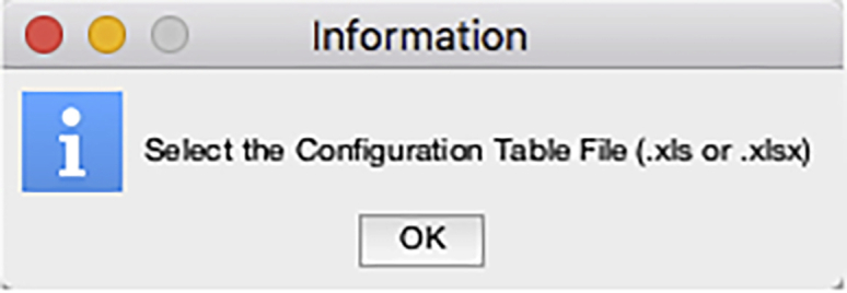
28.
A file Selection interface will then be displayed for the user to select the Configuration Table file (Figure 22).
Note: If the user clicks “Cancel” instead of selecting a file, a message will pop-up to give the options to abort the script or reselect a file.
-
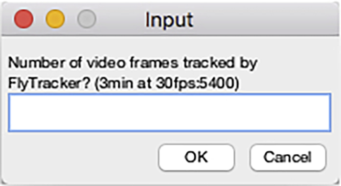
29.
A dialog box prompts the user to enter the number of video frames tracked with FlyTracker to be extracted (Figure 23).
Note: In general, we use the step 20 to restrict the analysis by FlyTracker to the first 3 min of video files and this step can be used to further reduce the number of frames to extract data from.
Note: This dialog box will prompt the user again if a non-numerical value is entered or if the “Cancel” button is clicked.
-
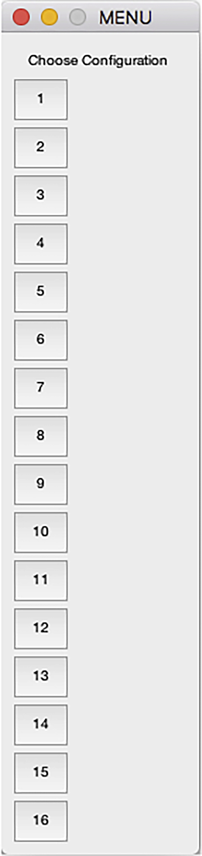
30.
A dialog box prompts the user to select the configuration used (Figure 24).
-
31.
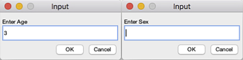
Dialog boxes prompts the user to enter the sex and age of the animals tracked (Figure 25).
-
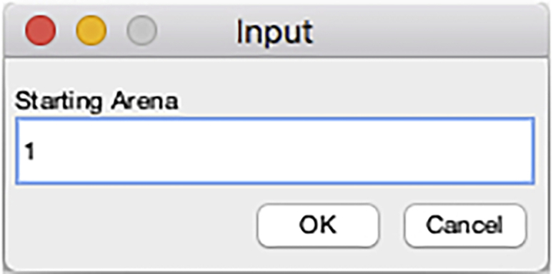
32.
A dialog box prompts the user to enter the number of the chamber (arena) to start to extract FlyTracker data (Figure 26).
Note: It may rarely happen that the tracking of one chamber is not satisfactory during the visual inspection with the visualizer in steps 22 and 23. In such case, FlyTracker analysis is re-run starting at step 10 and slight adjustments of the foreground and/or body threshold are applied. Such adjustment does not change the outcome of the tracking of the other chambers and this option can be used to save processing time.
-
33.
It may take a couple of minutes (dependent on the processing power of the computer used and the number of chambers tracked) before a file selection interface will prompt the user for the location to save the spreadsheet files with the extracted data (Figure 27).
Note: It is also possible to rename the files to be saved during this step.
-
34.
The script outputs two spreadsheet-compatible files (.csv and .xls) (Figure 28).
Figure 19.

Loading the DataExtractionScript and the two MATLAB structure array files
Figure 20.

The MATLAB interface after the loading of the DataExtractionScript and structure files
Figure 21.
Initial information displayed by the DataExtractionScript
Figure 22.

DataExtractionScript file selection interface to load the configuration table
Figure 23.
Video frames input dialog of the DataExtractionScript
Figure 24.
Configuration selection dialog of the DataExtractionScript
Figure 25.
Sex and age input dialogs of the DataExtractionScript
Figure 26.
Starting chamber input dialog of the DataExtractionScript
Figure 27.

DataExtractionScript file selection interface to save the output of the script
Figure 28.

The files output by the DataExtractionScript in the tracking folder directory
Data compilation
This step uses the DataCompilation script to combine in a single .xls file the results obtained in multiple .xls files.
-
35.
Create a Compilation folder with the .xls files generated by the DataExtraction script (Figure 29).
-
36.
Load the DataCompilationScript by dragging the file onto the MATLAB icon in the Mac OS dock or by using the “Open” button in MATLAB and select the file.
Note: The Script should open in the MATLAB Editor.
-
37.
Click the “Run” icon in the MATLAB Editor.
-
38.
A file Selection interface is displayed for the user to select the location of the Compilation folder.
Note: If the user clicks “Cancel” instead of selecting a folder or if the selected folder does not contain any .xls files, messages will pop-up to give the options to abort the script or reselect the folder.
-
39.
The script copies into a new table the labeled table from the first .xls file in the Compilation folder.
Note: For each subsequent .xls file, the script copies into the new table the unlabelled tables below the previous table.
-
40.
The new table is saved as “Compilation.xls” in the Compilation folder (Figure 30).
Note: The “Compilation.xls” name can be changed by modifying the line 32 of the DataCompilation script.
Figure 29.

Directory of the compilation folder after addition of video files
Figure 30.

The compilation file output by the DataCompilation script in the compilation folder directory
Expected outcomes
The outcome of this protocol is the output of a .csv file and a .xls file.
The .csv file contains the “flydata” extracted in an unlabeled table with rows corresponding to the video frames and four columns listing the x and y coordinates extracted from track.mat and the velocity and distance to the wall of the chamber extracted from feat.mat. The total number of columns is equal to the number of chambers tracked multiplied by four (Figure 31).
Figure 31.

Structure of the .cvs file output by the DataExtractionScript
The script adds at the bottom of the x coordinate columns the number of video frames tracked. At each iteration of the script the x and y coordinates are used to calculate distances travelled between two successive frames which are the summed up and added at the bottom of the y coordinate columns. The total distance travelled is important since it can affect average velocity. It should be noted that the instant velocity values between two frames calculated by FlyTracker are identical for the first two frames (frame 1 should not be calculable). Therefore the first frame velocity is excluded and the number of frames with velocities (velocity frames) is added at the bottom of the y coordinate columns. At each iteration of the script, when the velocity value is less than 1 (visual inspection of many videos established that the animal has not moved) the video frame is counted as an immobile frame and the velocity value is excluded. The number of immobile frames is added at the bottom of the velocity columns. Velocity values higher than 1 are summed and divided by the number of velocity frames minus the number of immobile frames to obtain the average velocity that is added at the bottom of velocity columns.
When opened with a spreadsheet software, the .csv file allows to quickly examine the trajectories in each chamber by plotting XY scatter graphs using the x and y coordinates columns (Figure 32).
Figure 32.

Fly trajectories plotted from the X and Y coordinates of the .cvs file output by the DataExtractionScript
The arrangement of the chambers is horizontally flipped because FlyTracker refers the pixel position in each video frame with the origin set at the top left corner. One can also easily use the “Distance to wall” columns to compute the position of the fly in the chamber in order to examine spatial preferences.
The .xls file contains a labeled table with as many rows as the number of chambers. The columns report the genotype/treatment, sex, age, chamber (arena) ID, number of video frames tracked, percent immobile (% of number of immobile frames out of number of velocity frames), total distance travelled (pixels) and the average velocity (mm/s).
There are many different ways to examine locomotor behavior in Drosophila with three well established methods: Trikinetics activity monitoring, climbing assays and video-assisted tracking. Trikinetics monitoring counts the number of infrared beam crossings and cannot be used to measure walking speed.11 Climbing assays measure spontaneous locomotion resulting from Drosophila natural negative geotactic behavior. However, most assays involve a mechanical stimulation of the fly that can affect behavior as well as walking speed, and are impractical to perform on single animals.12,13,14 The “fly vertically rotating arena for locomotion” (fly-VRL) is the most recent development in climbing assays that eliminate any forceful artificial stimulation and solely relying on the fly’s innate negative geotaxis.15 Nonetheless climbing assays measure climbing locomotion that requires more strength than walking, which may prevent the measurement of animals with weak muscles. Video-assisted tracking is widely used to measure locomotion.5,6,16,17,18 The FlyTracker software is highly versatile to analyze many aspects of Drosophila behavior and locomotion. Many possible protocols with modifications of the chambers and recording set-up can be designed around FlyTracker to examine specific parameters and the scripts provided with this protocol facilitate the processing of the data. For instance, the examination of spatial preference requires chambers with larger diameter and different geometry6 and it is clearly visible in the figure that the fly avoids the center in our chamber. Locomotion behavior can be examined in chambers ranging between 1.6 cm17 and 3.5 cm5 while spatial preference requires chambers ranging between 12.7 cm6 and 24.5 cm.16 This protocol is tailored to use FlyTracker to measure parameters that are most likely to be directly affected by muscle strength (how often the fly walk, how fast and how much distance is travelled) instead of parameters (spatial preference, changes of direction, legs coordination) that are also dependent on the activity of the nervous system.
Limitations
This protocol uses computer-assisted processing of video recordings to measure the locomotion of individual flies. A computer and a video camera are the sole hardware to be acquired that are easily accessible to any lab in any country and the locomotion device does not require any expenses (using leftover pieces of plexiglass, clear plastic or glass). Although any computer/camera can be used, the processing power of the computer and the resolution of the camera are the main limitations that needs to be considered. The resolution of the camera is limiting the number of individuals that can be tracked simultaneously. The higher the resolution the further the locomotion device can be from the camera, and the more individuals will be recorded simultaneously and tracked accurately. It is also important to take into account camera aberrations that may alter the shape of peripheral chambers (making them appeared elliptical instead of circular) in the video file. Camera aberrations are related to the hardware features of the camera itself and will increase with the size and/or number of chambers. With the camera we chose, although we lose the ability to track accurately if we use more than 50 chambers, there is no visible camera aberrations. A Python package has just been published that can be used to correct such aberrations but it will require additional computational steps to the workflow.17
Locomotion is a complex trait that is easily modifiable by the genetic background and environmental conditions.19 It is critical to ensure that the animals used are isogenic, and to avoid any change to the recording conditions (temperature, light, humidity). The effect of circadian rhythms on activity must be avoided by always recording at the same time of the day, ideally during the well-known morning period of activity. The culture (food composition, temperature, larval density) and collection/handling methods (mode of anesthesia, population density, frequency of food replacement) is well known to affect reproducibility. This protocol provides detailed descriptions of the culture and handling methods that are critical to achieve excellent reproducibility (Figures S1 and S2, Barwell et al.1).
Troubleshooting
Problem 1
FlyTracker fails to detect some flies or the detection is inaccurate.
Potential solution
This problem may arise if the locomotion device has fabrication defects (cracks in the plexiglass from drilling/cutting, gluing artefacts) that cause light shadowing artefacts that FlyTracker misidentifies. It is possible that the tuning of FlyTracker detection parameters (step 18) may help in some situations but we always found that the fastest solution is to use a different chamber or rebuild the device.
This problem will arise frequently if the video recording is done with cheap cameras and/or inappropriate lighting conditions (not enough or uneven lighting). The problem is easily identifiable at step 15 when FlyTracker displays the background-adjusted video. If the adjusted video is not obviously lighter than the original and the flies are not clearly distinguishable (or additional dark dots can be seen), no amount of tuning of FlyTracker detection parameters will help and the only solution is to re-record the video with the appropriate lighting.
Problem 2
MatLab crashes.
Potential solution
It is important during step 16 to avoid setting a chamber that does not contain a fly. FlyTracker should displays an alert when no fly is detected in a chamber but this feature has not been reliable for us and if this alert is not triggered, the software proceeds but the processing time slows down considerably and MatLab freezes often causing the computer to crash and restart.
Problem 3
FlyTracker cannot open the video file.
Potential solution
FlyTracker can open .mp4, .avi and .mv4 video formats. This problem randomly occurred with .m4v files and is easily fixed by replacing the .m4v extension by the .mp4 extension (step 7).
Resource availability
Lead contact
Further information and requests for resources and reagents should be directed to and will be fulfilled by the lead contact, Laurent Seroude (seroudel@queensu.ca).
Materials availability
This study did not generate new unique reagents.
Acknowledgments
This work has not received any funding from any source.
Author contributions
Conceptualization, T.B., L.S.; methodology, S.R., T.B.; writing, T.B., L.S.
Declaration of interests
The authors declare no competing interests.
Footnotes
Supplemental information can be found online at https://doi.org/10.1016/j.xpro.2022.101888.
Contributor Information
Taylor Barwell, Email: 9teb4@queensu.ca.
Laurent Seroude, Email: seroudel@queensu.ca.
Data and code availability
The protocol did not generate/analyze datasets.
All original code has been deposited at Zenodo and is publicly available as of the date of publication. DOIs are listed in the key resources table.
References
- 1.Barwell T., Raina S., Seroude L. Versatile method to measure locomotion in adult Drosophila. Genome. 2021;64:139–145. doi: 10.1139/gen-2020-0044. [DOI] [PubMed] [Google Scholar]
- 2.Ashburner M., Golic K.G., Hawley R.S. In: Drosophila: A Laboratory Handbook. Inglis J., editor. Cold Spring Harbor Laboratory Press; 2005. Life cycle; pp. 121–205. [Google Scholar]
- 3.Bidaye S.S., Laturney M., Chang A.K., Liu Y., Bockemühl T., Büschges A., Scott K. Two brain pathways initiate distinct forward walking programs in Drosophila. Neuron. 2020;108:469–485.e8. doi: 10.1016/j.neuron.2020.07.032. [DOI] [PMC free article] [PubMed] [Google Scholar]
- 4.Howard C.E., Chen C.L., Tabachnik T., Hormigo R., Ramdya P., Mann R.S. Serotonergic modulation of walking in Drosophila. Curr. Biol. 2019;29:4218–4230.e8. doi: 10.1016/j.cub.2019.10.042. [DOI] [PMC free article] [PubMed] [Google Scholar]
- 5.Schretter C.E., Vielmetter J., Bartos I., Marka Z., Marka S., Argade S., Mazmanian S.K. A gut microbial factor modulates locomotor behaviour in Drosophila. Nature. 2018;563:402–406. doi: 10.1038/s41586-018-0634-9. [DOI] [PMC free article] [PubMed] [Google Scholar]
- 6.Simon J.C., Dickinson M.H. A new chamber for studying the behavior of Drosophila. PLoS One. 2010;5:e8793. doi: 10.1371/journal.pone.0008793. [DOI] [PMC free article] [PubMed] [Google Scholar]
- 7.Bartholomew N.R., Burdett J.M., VandenBrooks J.M., Quinlan M.C., Call G.B. Impaired climbing and flight behaviour in Drosophila melanogaster following carbon dioxide anaesthesia. Sci. Rep. 2015;5:15298. doi: 10.1038/srep15298. [DOI] [PMC free article] [PubMed] [Google Scholar]
- 8.Shen J., Yang P., Zhu X., Gu Y., Huang J., Li M. CO2 anesthesia on Drosophila survival in aging research. Arch. Insect Biochem. Physiol. 2020;103:e21639. doi: 10.1002/arch.21639. [DOI] [PubMed] [Google Scholar]
- 9.Eyjolfsdottir E., Branson S., Burgos-Artizzu X.P., Hoopfer E.D., Schor J., Anderson D.J., Perona P. Detecting social actions of fruit flies. Lect. Notes Comput. Sci. 2014;8690:772–787. [Google Scholar]
- 10.Arking R. Fourth edition. Oxford University Press; 2018. Biology of Longevity and Aging: Pathways and Prospects. [Google Scholar]
- 11.Chiu J.C., Low K.H., Pike D.H., Yildirim E., Edery I. Assaying locomotor activity to study circadian rhythms and sleep parameters in Drosophila. J. Vis. Exp. 2010 doi: 10.3791/2157. [DOI] [PMC free article] [PubMed] [Google Scholar]
- 12.Cao W., Song L., Cheng J., Yi N., Cai L., Huang F.D., Ho M. An automated rapid iterative negative geotaxis Assay for analyzing adult climbing behavior in a Drosophila model of neurodegeneration. J. Vis. Exp. 2017 doi: 10.3791/56507. [DOI] [PMC free article] [PubMed] [Google Scholar]
- 13.Gargano J.W., Martin I., Bhandari P., Grotewiel M.S. Rapid iterative negative geotaxis (RING): a new method for assessing age-related locomotor decline in Drosophila. Exp. Gerontol. 2005;40:386–395. doi: 10.1016/j.exger.2005.02.005. [DOI] [PubMed] [Google Scholar]
- 14.Spierer A.N., Yoon D., Zhu C.T., Rand D.M. FreeClimber: automated quantification of climbing performance in Drosophila. J. Exp. Biol. 2021;224:jeb229377. doi: 10.1242/jeb.229377. [DOI] [PMC free article] [PubMed] [Google Scholar]
- 15.Aggarwal A., Reichert H., VijayRaghavan K. A locomotor assay reveals deficits in heterozygous Parkinson's disease model and proprioceptive mutants in adult Drosophila. Proc. Natl. Acad. Sci. USA. 2019;116:24830–24839. doi: 10.1073/pnas.1807456116. [DOI] [PMC free article] [PubMed] [Google Scholar]
- 16.Branson K., Robie A.A., Bender J., Perona P., Dickinson M.H. High-throughput ethomics in large groups of Drosophila. Nat. Methods. 2009;6:451–457. doi: 10.1038/nmeth.1328. [DOI] [PMC free article] [PubMed] [Google Scholar]
- 17.Qu S., Zhu Q., Zhou H., Gao Y., Wei Y., Ma Y., Wang Z., Sun X., Zhang L., Yang Q., et al. EasyFlyTracker: a simple video tracking Python package for analyzing adult Drosophila locomotor and sleep activity to facilitate revealing the effect of psychiatric drugs. Front. Behav. Neurosci. 2021;15:809665. doi: 10.3389/fnbeh.2021.809665. [DOI] [PMC free article] [PubMed] [Google Scholar]
- 18.Valente D., Golani I., Mitra P.P. Analysis of the trajectory of Drosophila melanogaster in a circular open field arena. PLoS One. 2007;2:e1083. doi: 10.1371/journal.pone.0001083. [DOI] [PMC free article] [PubMed] [Google Scholar]
- 19.Martin J.R. Locomotor activity: a complex behavioural trait to unravel. Behav. Processes. 2003;64:145–160. doi: 10.1016/s0376-6357(03)00132-3. [DOI] [PubMed] [Google Scholar]
Associated Data
This section collects any data citations, data availability statements, or supplementary materials included in this article.
Supplementary Materials
Data Availability Statement
The protocol did not generate/analyze datasets.
All original code has been deposited at Zenodo and is publicly available as of the date of publication. DOIs are listed in the key resources table.