

Abstract
Experiments using conventional experimental approaches to capture the dynamics of ion channels are not always feasible, and even when possible and feasible, some can be time-consuming. In this work, the ionic current–time dynamics during cardiac action potentials (APs) are predicted from a single AP waveform by means of artificial neural networks (ANNs). The data collection is accomplished by the use of a single-cell model to run electrophysiological simulations in order to identify ionic currents based on fluctuations in ion channel conductance. The relevant ionic currents, as well as the corresponding cardiac AP, are then calculated and fed into the ANN algorithm, which predicts the desired currents solely based on the AP curve. The validity of the proposed methodology for the Bayesian approach is demonstrated by the R (validation) scores obtained from training data, test data, and the entire data set. The Bayesian regularization’s (BR) strength and dependability are further supported by error values and the regression presentations, all of which are positive indicators. As a result of the high convergence between the simulated currents and the currents generated by including the efficacy of a developed Bayesian solver, it is possible to generate behavior of ionic currents during time for the desired AP waveform for any electrical excitable cell.
Supplementary Information
The online version contains supplementary material available at 10.1007/s10867-022-09619-7.
Keywords: Cardiac action potential, Artificial neural networks, Bayesian regularization, Numerical modeling, Current–time dynamics
Introduction
Using ANNs has opened up new horizons in several disciplines of medicine during the last few years, including biophysics [1], systems biology [2], and pharmacology [3], among many others [4]. One of the driving forces behind this improvement has been the ability to handle vast amounts of data and form conclusions based on characteristics that are difficult to describe and evaluate using linguistic forms, which has allowed for significant advancement. Using ANN algorithms, raw features from a massively huge, structured data set, such as a set of curves or images, can be used to develop an automated forecasting tool that is based on patterns hidden within the data set [5]. Once taught, the algorithms can use that knowledge to analyze other data, which can come from a variety of sources, some of which are diametrically opposed to one another. In spite of the fact that rodents and humans exhibit very nonlinear electrophysiological behaviors that are distinct from one another, such as the difference in the It density and high magnitude of It in rat/mouse than human, which causes the rat and mouse hearts to have a large initial repolarization phase and a short/lack plateau phase at a lower membrane potential than humans [6], the idea being discussed here is not model or species specific. In the medical literature, there is a mathematical model of the human cardiac AP, and an analogous ANN analysis may be carried out on the dynamics of the human heart in conjunction with the dynamics of the human channels. In this way, some of the inherent limitations of humans may be overcome, resulting in ANN becoming a helpful tool that can be used in conjunction with established methodologies in theoretical and experimental medicine to produce beneficial results [4, 7, 8].
Biological neural networks inspired ANN networks and they can solve a lot of issues in pattern recognition [9, 10], prediction [11], and optimization [12] including associative memory [13]. The optimization of ion channel dynamics is another area where ANN can be used successfully. Ion channels are transmembrane proteins with pores that permit ions to diffuse down an electrochemical gradient. Ion channels have several functions in the body, but one of the most important is in the cardiovascular system, where the passage of potassium, sodium, and calcium ions across cardiomyocytes is essential for maintaining a regular heart rhythm. In order to provide mechanistic insight into a range of electrophysiological processes, computational simulations and mathematical modeling have shown to be quite beneficial [14–16]. Ion channel mathematical models are essential components of these AP models. For calibrating ion channel models, voltage-clamp experiments are a frequent source of data. Whittaker et al. [17] went into detail about how calibrating the parameters of ion current and action potential (AP) models to experimental data sets is a crucial step in building a predictive model. They also talked about the many problems that the work done so far has brought up, as well as the need for repeatable descriptions of the calibration process so that models can be re-calibrated to new data sets and built on for future studies. Models are simulated according to the best available data but it is not always possible to find data for each ionic current. Even when models are fitted to the best available data, since recording each current from the same cell is nearly impossible there is still uncertainty in parameter values due to this measurement ambiguity and/or physiological variability. In recent years, statistical methods have been developed and used in many scientific fields to capture uncertainty in the quantities that determine how a model works and to create a distribution of predictions that takes this uncertainty into account. Johnstone et al. [18] take uncertainty quantification into account for cardiac electrophysiology models. They also point out how important it is that cardiac myocytes have a lot of observational uncertainty and natural variability. Knowing the dynamics of each ionic current and AP from the best available data without doing experiments each time would be very useful for excitable cell research. As a pilot research, this investigation makes use of a Bayesian technique to predict the current–time curves of cardiac dynamics derived from AP curves. A wide variety of Bayesian algorithms have been applied in medicine [19–21]. In the Bayesian method, regularization is accomplished by first setting a prior distribution over the parameters and then averaging over the posterior distribution. This procedure is repeated until the desired effect is obtained. This regularization helps influence the selection of model structures in addition to providing smoother estimates of the parameters than maximum likelihood does [22, 23].
Changes in ion channel conductance can affect APs due to a variety of factors like as mutations or medications. APs have been anticipated using advanced studies based on alterations in certain ion channels. Luo and Rudy [24] employed a mathematical dynamic model to anticipate variations in ionic currents and APs in ventricular cells based on intracellular Ca2+ concentration variations. Using a computer model, Akanda et al. [25] predicted changes in APs due to biochemical changes produced by toxic medications, and hypothesized that drug toxicity or impacts can be identified by studying APs. From the calculated AP difference shapes, Jeong and Lim [26] were able to make a prediction about the changing ion channel conductance. Specific ionic conductances were classified in their studies based on AP shape differences. Despite the use of ANN in both research, no regression analyses have been performed so far that forecast all current–time curves based on a single AP form, as we aimed in our study. Recently, Şengül et al. [27] modeled the cardiac AP with the best available data and analyzed the pathological situations. It is reported in this research that data for IK1, IKr, and IKs was not available in the literature and the available data was from different cells in different researches. This work will be the pilot study to overcome the forecasting of different mutations and absent ion channel dynamics. A single-cell model is used to perform electrophysiological simulations to determine ionic currents based on ion channel conductance fluctuations. In the AP simulation, we alter the conductance of each ion channel by raising or lowering it at a constant rate, which ultimately produces 880 different AP types. Then, during the AP, the relevant ionic currents are calculated and the results are fed into the machine learning model to anticipate the desired current. Perturbed data is used to simulate mutations to train our network and calculate the time vs the ionic current curves from the given AP curve by using ANNs.
Model simulation
In cardiomyocytes, APs are generated in five stages, each of which consists of a major ion channel that causes a shift in membrane potential. In a resting state, potassium (K+) channels maintain the cell’s membrane potential at a steady negative potential (phase 4). In the phase 0, the sodium (Na+) channel opens when the cell’s membrane potential reaches the threshold potential of around − 65 mV, and as sodium ions enter the cell from the outside, the membrane potential changes quickly from negative to positive, creating an upstroke (phase 1). It causes the Na+ channel to become inactive while simultaneously activating the K+ channel. The inward Ca2+ current and outward K+ current then approach a plateau as the calcium (Ca2+) channel and delayed rectifier K+ outward channel is opened (phase 2). As the Ca2+ channel is deactivated, the cell’s membrane potential, which was previously positive, returns to a level near to the K+ equilibrium potential. The outward K+ channel is then closed, whereas the inward K+ channel is opened (phase 3). Finally, due to the inward K+ current, it returns to the perfectly stable state of phase 4.
The training data used for ANN were obtained using Şengül et al. [27] ’s single-compartment electrophysiological ventricular cell model. It is possible to express the membrane voltage in terms of the sum of 12 currents and three ion transporters that pass across the membrane, as follows:
| 1 |
with a capacitance of the membrane and an external applied current .
The following formula describes all of the ionic currents in the model:
| 2 |
In this equation, Y denotes the relevant ion channels, and denotes the maximum conductance of the channel for the reversal potential Eion (ion = Na+, Ca2+, K+, Cl−). In this equation, a, b, and c indicate activation, fast inactivation, and slow inactivation gating variables (if any are present), respectively. The integer powers of those gating variables are represented by the letters M, N, and L. Each voltage-dependent gating variables x, related steady-state functions , and time constants are represented by Eq. (3).
| 3 |
In the approach described here, maximum conductances () will be disturbed, and the changes in the output on the time vs AP curve and the changes in the output on the time vs current curves will be generated as a data set for further analysis. The Bobyqa, Newuoa, and Cobyla algorithms are used to find the best values for all of the channels’ maximum conductances based on the AP recordings. Next, the 32nd order Nonlinear Differential Equation System (NDE) is solved by using all of the parameters that have been optimized using Gear’s method, which changes the step size to its best value with each iteration. This equation generates 880 different AP waveforms and associated current curves based on the conductances of 12 ion channels, and Fig. 1 illustrates the APs and Fig. 2 shows the accompanying some current–time curves throughout the duration of a 50 to 150 ms cycle.
Fig. 1.

A description of the ANN design for the BR algorithm
Fig. 2.
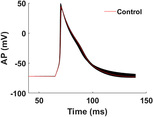
AP waveforms that were generated through simulation after conductances were altered. The model receives these curves as inputs and processes them accordingly
Data preprocessing
Obtaining the data set was the first step in our preprocessing stage. This was accomplished by simulating the model using Eqs. 1, 2, and 3. In the first step of this process, we altered the values of all 12 maximal conductances by looking at their oscillatory regions. In general, Hopf or saddle-node of periodics (SNP) bifurcations are what delimit the parameter interval for oscillations (Şengül et al. [28]). That is to say, when one of the parameters in a model is changed, the model will start to oscillate and will stop oscillating based on one of these bifurcations. Therefore, it was necessary for us to examine the oscillatory area of the action potentials, and the waveforms of these APs must not deviate from the waveforms that are characteristic of a cardiac AP. Before beginning the training process, both the AP curves as an input and the current–time curves as target data sets are evaluated for values that are corrupt, constant, or inaccurate.
After ensuring that there are no nonphysiological or incorrect AP data, we realized that the dimension of the input vector could be a significant factor in determining how effectively the training is carried out. There are some situations in which the dimensions of the data vectors might be relatively big, but the components of the data vectors might demonstrate a high degree of correlation despite this fact. Therefore, duplicate AP curves and the currents that are associated with them are cleared. At this point, we have come to the conclusion that because our system is nonlinear, distinct ionic conductance perturbations can produce AP waveforms that are visually identical to one another. Because of this, we sought to place our attention on the primary currents that had the greatest impact on the AP waveform and get the best possible approximation while using the smallest amount of data as feasible. Because each category of ionic current has an effect on a different stage of the AP waveform, the Na+, K+, Ca2+, and background Cl- currents that have the most impact on the waveform are selected from within each category in addition to the membrane capacitance Cm which plays a role in the AP waveform as a coefficient of the voltage change and perturbation (as seen in Eq. 1). The fast depolarization, or phase 0 of the cardiac AP, is driven by Na+ current (INa), and this in turn activates ICaL in a voltage-dependent manner, as validated by Sırcan and Şengül’s [38] quantitative measurements of the functions of ion channel dynamics on the focused model. The data also provides quantitative evidence for the predominance of It activation during early repolarization, ICaL activation during the plateau phase, and It activation once more during the late repolarization phase. The conductance values listed in Table 1 are displaced within the bounds indicated due to the contribution analysis and the regions of the oscillations.
Table 1.
Perturbed conductance values in (nS/pF) together with the membrane capacitance in (pF) and range to create the data set
| Parameter | Description | Control value | Minimum | Maximum |
|---|---|---|---|---|
| gNa | Fast Na+ current conductance | 3758.5 | 2500 | 7250 |
| gCaL | L-type Ca2+ current conductance | 10.06 | 7.9 | 12.325 |
| Cm | Membrane capacitance | 100.0 | 95 | 104.971 |
| gClb | Cl− background conductance | 0.25953 | 0.24 | 0.3099 |
| gt | Transient K+ current conductance | 9.197 | 9.1 | 10.05 |
A total of 880 distinct AP waveforms and current curves are created as a data set after utilizing a grid search and clarification of the redundant data. Gear’s Method is used in the MATLAB environment to solve the 30-s order Nonlinear Differential Equation System with all of the altered conductances in order to obtain a data set of results.
The Bayesian regularization algorithm
In order to train and evaluate our cardiac AP dynamics, we employed the BR approach in conjunction with the MATLAB programming language and numeric computing environment offered by MathWorks. Using Hessian-based approaches, the network may learn more exact aspects of a complicated mapping, allowing it to become more accurate. Hessian-based Levenberg–Marquardt (LM) algorithms for nonlinear least squares problems were invented by Levenberg and Marquardt, who were the first to propose them. As part of the Lagrangian minimization optimization, the BR technique modifies the weight and bias values of the network training function.
For a network to generalize successfully, it must first minimize a combination of squared errors and weights, after which it must determine the best combination of these parameters to get the lowest possible error. The following are the stages of the algorithm, summarized as follows:
In step 0, the objective function parameters are initialized, as well as the weights. Foresee and Hagan [29] select to set α = 0 and β = 1 and to initialize the weights using the Nguyen-Widrow approach as described in Nguyen and Widrow [30]. It is expected that the objective function parameters would return to their original values after the first training phase.
In step 1, one step of the LM algorithm is performed to minimize the objective function according to Eq. 4;
| 4 |
where denotes the vector of network weights, denotes the sum of squared errors, and denotes the sum of squares of the network weights.
In step 2, the effective number of parameters is computed as Eq. 5
| 5 |
where is the total number of parameters in the network and is the Hessian available in the LM algorithm which can be described with Eq. 6:
| 6 |
Here, is the Jacobian matrix of the training set errors, is the identity matrix of size N.
In step 3, the new estimates for the objective function parameters are computed as Eq. 7,
| 7 |
As a step 4, steps 1 through 3 are performed until convergence is reached.
All supplied data sets are dispersed in a random manner for training and testing in order to get the highest degree of convergence. In this scenario, we picked the sets such that 85% of the data would be used for training and 15% of the data would be used for testing the model. The number of neurons is likewise variable; as demonstrated in Fig. 1, network of 2–10-13 produces acceptable computational results. In this case, the information on the time as well as the value of the voltage is included inside two inputs. A hyperbolic tangent activation function is taken into consideration while working with the 10 neurons that are applied in the hidden layer. On the other hand, for the output layer, we employed a linear activation function and used 13 neurons. As a consequence of this, thirteen different ionic current–time curves are estimated based on the information about time and voltage input.
Results
We used a machine learning method with ANN layers to predict the current–time curves of ion channels based on cardiac AP shapes in this study. Cell electrophysiological modeling is used to create the AP, based on changes in 12 ion channels.
A total of 880 distinct AP waveforms and current curves are created as a data set for our ANN algorithm using four conductance values and one membrane conductance that are modified with a constant step from minimum values to maximum values as shown in Table 1. Figure 2 depicts the cardiac APs that occur within a single spike interval that ranges from 50 to 150 ms, as determined by the fluctuation in ion channel electrical conductances. Figure 2 shows the AP curves, which are inputs to our model, and Fig. 3 shows the current–time dynamics, which are outputs. The AP curve and the associated current–time dynamics are illustrated in red when there has been no change in the ion channel conductance, which occurs in the control condition. Black curves are the results of the simulation. Once we look at the changes in phases due to the perturbation of the specified conductances, with the exception of IK1 (Fig. 3G) and IClb (Fig. 3N), variations in conductance levels did not result in any substantial changes in phase 0 of any of the currents (Fig. 3). We detected substantial changes around the peak points of the graphs (i.e., in phase 1) of almost all currents mostly ICaPp (Fig. 3J). In phases 2 and 3, the graphs of ICaPp (Fig. 3H) and INaKp (Fig. 3J) show the greatest variance, respectively. When it comes to phase 4, the values of ICaL (Fig. 3B), IKr (Fig. 3E), IKs (Fig. 3D), INa (Fig. 3A), and It (Fig. 3F) are extremely close to zero. IK1 (Fig. 3G), and INaKp (Fig. 3J) exhibit the greatest amounts of fluctuation during phase 4. In addition, the Na+, K+, and Ca2+ background currents, in conjunction with the funny current Ihf, have the greatest influence on phases 3 and 4, as illustrated in Fig. 3K, L, M, and O, respectively. The fact that the rate of change from a single modification is often greater than the rate of change from a smaller scale of current values is worth mentioning. An extreme situation is given in Fig. 3A, where it is difficult to discern without zooming in if the Na+ current is at zero mA in phases 0 and 4 due to how high the peak value is in relation to the rest of the current. As an opposite situation, certain current curves such as IK1, INaCaP (Fig. 3I), and ICaT (Fig. 3C) are not robust, meaning they are extremely sensitive to variations in the conductances of the circuit because they have smaller amplitude. Modifications to their conductances that are quite minor can result in significant shifts in their current curves as shown in Fig. 3C, G, and I.
Fig. 3.

A through O illustrate the outcomes of the simulation following the application of the perturbations to channel conductances. The control currents are shown by the red lines in the illustration. Here, A INa is Na+ current, B ICaL is L-Type (long-opening) Ca2+ current, C ICaT is T-Type (transient) Ca2+ current, D IKs is slowly activated outward rectifier K+ current, E IKr is rapidly activated outward rectifier K+ current, F It is transient outward K+ current, G IK1 is inward rectifier K+ current, H INaKp is Na+-K+ pump current, I INaCap is Na+-K+ exchanger (NCX) current, J ICap is sarcolemmal Ca2+ pump current, K INab is Na+, L ICab is Ca2+, M IKb is K+, N IClb is Cl− background currents, and O Ihf is hyperpolarization-activated current
The numerical findings of ion channel dynamics that have been modeled from a single AP as a consequence of an ANN algorithm are displayed in the figures and tables that can be found below. In Fig. 4, we provide one random simulation result, as determined in Eq. (1) through (3), together with the relevant fitting results from the BR technique. These findings are shown in conjunction with the random simulation result as shown in Na+ current (Fig. 4A), L-type Ca2+ current ICaL (Fig. 4B), slowly activated outward rectifier K+ current IKs (Fig. 4D), rapidly activated outward rectifier K+ current IKr (Fig. 4E), transient outward K+ current It (Fig. 4F), Na+-K+ pump current INaKp (Fig. 4H), sarcolemmal Ca2+ pump current ICaPp (Fig. 4J), background currents (Fig. 4K–N), and hyperpolarization-activated current Ihf (Fig. 4O). The complete set of findings from the fittings is presented in Figure S1. For each ionic current, a random set of parameters is chosen to generate the AP (shown in red) and the BR prediction (shown in blue). We can see that BR gives an accurate fitting that almost overlaps the true functions in the majority of the domain, but deviates somewhat in particular intervals. The smaller amplitude currents like INaCaP (Fig. 4I) and ICaT as we mentioned before showed the biggest variability from the real behavior as shown in Fig. 4C and I, respectively. The noisy behavior of the ICaT (Fig. 4C) current is caused by a large discrepancy in the ICaT training set, as seen in Fig. 3C. However, the noise is visible around the real current curve, and a smooth filter may be used to remove the noise after the regression, allowing us to obtain the focused current–time curves more precisely at the end.
Fig. 4.

Predictions for one cell (2000 rows) resulting from one set of AP. A The AP. B–I show the currents. Red dots and blue dots represent the real values and the predictions, respectively
The performance interpretation of ANN computing is explained in detail in Table 2 and regression plots with R scores are given in Figure S2. For a total of 12 ionic currents, the mean absolute errors (MAE), relative mean squared errors (RMSE), and mean percentage errors are calculated together with the R2 values as in Table 2. All of the currents, with the exception of INaCaP, exhibit an R2 value of greater than 0.9, which indicates that the model results are highly correlated with the true values and the fitting findings are satisfactory. In addition, as shown in Fig. 4, all of the channel findings have MAE and RMSE values that are within acceptable ranges. As can be seen in Figs. 4 and S1, the MPE outcomes are proportional to the current amplitudes, with larger amplitudes yielding more MPE results. The difficult fitting work is made more difficult by the smaller amplitude, distorted shape, noise, and many peaks of curves. The INaCaP current serves as a good example of this, and its R2 value of 0.7409938561 is the lowest of all the currents. This indicates that the network that was obtained may explain around 74% of the data that was observed. Although the Na+ current curve has the highest RMSE value because of the late Na+ bump and an amplitude reaches to 15000pA, the smaller MAE value and 0.9988 R2 value show the accurate fit for this channel. The ICaT revealed variability from the true data from the figures as well, but the value of R2 was 0.9816648241, which indicates that the results are acceptable.
Table 2.
Mean absolute error, relative mean squared error, mean percentage error, and R2 values of the modeled ionic currents
| Parameter | MAE | RMSE | MPE | R2 |
|---|---|---|---|---|
| INa | 5.7238 | −9.2992 | −42,628.9293 | 0.9988603249 |
| ICaL | 2.6942 | −0.7880 | −1187.5453 | 0.9970621609 |
| It | 4.6057 | 0.6539 | 501.1568 | 0.9982807396 |
| IKs | 2.0029 | 0.2753 | 761.172 | 0.9966228561 |
| IKr | 0.20609 | 0.3374 | 222.5513 | 0.954529 |
| IClb | 0.63994 | −0.2022 | −4.4775 | 0.9904429441 |
| ICap | 6.4926 | 1.1387 | 27.5906 | 0.9842227264 |
| INaKp | 0.0072715 | 1.4756e − 05 | 0.099072 | 0.9972818496 |
| IK1 | 3.4573e − 05 | 1.0456e − 06 | 9.6490e + 46 | 1 |
| ICaT | 0.0027 | −0.006 | −49.1127 | 0.9816648241 |
| INab | 0.5543 | −0.0126 | −1.2858 | 0.9962435344 |
| IKb | 0.4163 | 0.0349 | 8.1093 | 0.9961437249 |
| ICab | 0.10156 | −0.0023 | −1.2694 | 0.9960439204 |
| Ihf | 0.0088177 | −0.0021 | 9.6428 | 0.9951858081 |
| INaCap | 0.63994 | −0.0028 | −145.8277 | 0.7409938561 |
It is important to note that Fig. 4G demonstrates that during a significant portion of the AP, the amplitude of the IK1 current approaches zero to such a degree that the naked eye is unable to discern significant differences without the use of magnification. On other occasions, the order of magnitude is no higher than 10−2. If the maximum amplitude of IK1 had been of a bigger order of magnitude, comparable to, for example, the situations of INa and ICaL, the ANN would have been able to generate predictions with a higher degree of precision. Because of the lack of robustness, the majority of IK1 values are treated the same when calculating the best fit for the regression. As a result, the line of best fit for the regression of IK1 exhibits a misleading perfect fit, as can be seen in Fig. 5A and B. As shown in Fig. 5C, the order of magnitude of a data point for IK1 and what the ANN predicted for it are in the range of 10−36 and 10−6, respectively.
Fig. 5.

A False perfect fit for IK1 regression. B The predictions for one cell, which has 2000 rows, based on one particular set of AP. The measured (numerical) values are represented by the red dots, and the predictions are shown by the blue dots (although it may be difficult to see them without zooming in C). Zoomed in on the time area that occurs between 78 and 78.6 ms during an IK1 simulation and the ANN’s prediction for it
Discussion
In this pilot study, the results presented here show that ion channel dynamics may be predicted from single AP waveforms using structural data generated from conductance-based differential equation models. Located in the plasma membrane, ion channel receptors extend between the two sides of the membrane to form pores that are called ion channels. Ion channels vary considerably in the factors that make them open or close, which comprises their gating [31]. Some are activated when substances such as neurotransmitters or cytoplasmic messenger molecules are present in the environment. Some are activated by variations in the voltage across the cell wall, while others are opened by different types of sensory stimulation. When it comes to the ions to which they are permeable, channels are quite selective. Some of them allow just certain ions to flow through, while others are selective for wider types of ions, such as monovalent cations, while others are indifferent [31]. Each channel shows a different behavior in its response to time-varying input.
We are able to notice patterns in the graphs of the currents formed by the passage of these ions as a consequence of the mathematical models that have been developed via the use of real data. These patterns may be seen when voltage-gated channels and the ions that they allow to flow are utilized. When using mathematical models and simulations to make decisions, it is very important to measure uncertainty and model the differences. In the field of cardiac simulation, people have started to look for and use ways to describe how uncertainty in model inputs spreads to outputs or predictions [17, 18, 32]. Our approach will be a big help in figuring out how these unknowns and changes affect the output of the current dynamics. We developed an ANN algorithm using these patterns to see how well we can forecast the variable behavior of channels and the uncertainties as a result of conductance perturbations. We decided to go with the BR way of fitting. Following a number of iterations consisting of both success and failure, we determined that the optimal number of sets is 880, which corresponds to 1,760,000 rows of data. Including additional cells did not result in any positive outcomes. On the other hand, reducing the number of cells brings the prediction percentage down to a lower level.
The first method, known as the scaled conjugate gradient (SCG) methodology, was developed specifically for use in supervised learning applications like ANN. SCG, in contrast to existing second-order algorithms, does not require a time-consuming line search for each learning iteration, resulting in a speedier algorithm than existing second-order algorithms. In other words, SCG is an improvement over existing second-order algorithms [33]. On the other hand, the precision of this method cannot be tolerated when working with massive data sets like the one that we are working with. According to the literature, Levenberg–Marquardt (LM) and Bayesian regularization (BR) are capable of obtaining fewer mean squared errors than any other approach for functional approximation issues Demuth and Beale, [34]. To reduce estimating errors and establish a good generalized model, BR features an objective function that comprises a residual sum of squares and the sum of squared weights [35–37]. Several studies have been conducted to compare the predictive capacities of LM and BR, with the benefit of BR being its capacity to show potentially complicated correlations. We also used the LM method with both 12 conductance perturbation and preprocessed data with 5 parameters, and BR performed better in both cases.
It can be observed that, just as one would anticipate with any ANN technique, the efficiency of the model improves as the data range is larger, and the model can catch all the changes in the curve. However, if the data are only moving within a narrow range, the models would not be able to accurately anticipate the changes. Within our model, there are specified to be 12 ion channels that have a direct nonlinear influence on the myocytes of the left ventricle. On the other hand, the dynamics of some background channels, such as INaB, are shifting in the 0.1 mV range. We have found that the predictions made by ANN using these channels are insufficient. However, the dynamics of the main channels that make significant contributions to the AP are capable of being predicted with a high level of R2 values. The contributions of the channels are computed in (Sırcan and Şengül Ayan [38]), and this research takes into consideration the contributions of all significant channels that have an influence on the AP form. With R2 values of more than 0.9, the current–time curves of eight different channels were able to be predicted based on the AP waveform.
Ion channels that have larger amplitudes can be accurately predicted from a single AP curve, as can be shown in the findings; however, it is difficult to accurately estimate currents that have a magnitude of less than 1pA since the magnitude of these currents is already so small. What we can do about it is, before feeding it into the algorithm, we can raise the magnitude of the current by a fixed ratio, and then at the conclusion of the prediction, we can drop this current by the same ratio. As a result of the fact that the behavior of the curve will not be altered, this can safeguard the model against numerical inaccuracies as well as incorrect predictions.
The classical inverse problem might be used as another method to this current–time dynamic modeling. By considering all cardiac AP voltage waveform, the best parameters of current dynamics in Eqs. 1, 2, and 3 can be predicted by bringing the R2 value closer to one, as attempted before for different models [17, 32]. Uncertainties in the quantities such as maximal conductance that determine model behavior for cardiac cells is also studied by Johnstone et al. [18].
Moreover, it is not strictly necessary for neural networks to learn in order to perform normalization or scaling, but doing so greatly aids the learning process by transforming the features and output into the range in which the sigmoid activation functions operate. All curves in our study are normalized to a range of [0,1] and standardized to rescale the curves so that their data have a mean of 0 and a standard deviation of unit variance separately. Training and testing procedure is also applied to these data separately. We compared the R2 values and the MAE to the original scores, and while the results were somewhat better for certain channels (IKr, IKs, ICaT), they were either worse or equivalent for the remaining channels.
We think that AP waveforms from different cells may be fed into an ANN system, and that subsequent research could try to foresee important channel dynamics based on the AP waveform. With just an 880 AP waveform, we were able to make an accurate prediction of the current–time dynamics of ventricular cardiac AP from a single AP waveform. Therefore, the database is able to be created with the interested AP waveforms from various electrically excitable cells, such as neurons, cardiac cells, and muscle cells, belonging to various species, such as rats, mice, pigs, and humans, together with their various dynamics, such as steady-state activation-inactivation curves and time constants. Because our model does not have a very wide parameter range, we were forced to employ a tight parameter range in order to maintain the AP in a form that is physiologically relevant. Since this is just a pilot project, more robust models with wider parameter regions will need to be employed in order to generate the database, but an analogous ANN technique will still be able to be used to predict the dynamics of interest. After this database has been trained, the only thing that the researcher has to do is feed the AP waveform to the algorithm, and then machine learning may be used to predict all of the important ion channel dynamics. As a result, there is no longer a requirement to conduct experiments each time.
Supplementary Information
Below is the link to the electronic supplementary material.
Author contribution
SSA, SS, and HÖ designed the studies; SSA and SS performed simulation, SSA and HÖ analyzed the data; SSA and SS wrote the paper. All authors have seen and approved the final version of the manuscript.
Declarations
Ethical approval
This research does not need an ethical approval.
Conflict of interest
The authors declare no competing interests.
Informed consent
Informed consent is not applicable to this research.
Footnotes
Publisher's Note
Springer Nature remains neutral with regard to jurisdictional claims in published maps and institutional affiliations.
Contributor Information
Sevgi Şengül Ayan, Email: sevgi.sengul@antalya.edu.tr.
Selim Süleymanoğlu, Email: selim.suleymanoglu@std.antalya.edu.tr.
Hasan Özdoğan, Email: hasan.ozdogan@antalya.edu.tr.
References
- 1.Van de Burgt Y, Gkoupidenis P. Organic materials and devices for brain-inspired computing: from artificial implementation to biophysical realism. MRS Bull. 2020;45(8):631–640. doi: 10.1557/mrs.2020.194. [DOI] [Google Scholar]
- 2.Hall LM, Hill DW, Menikarachchi LC, Chen M, Hall LH, Grant DF. Optimizing artificial neural network models for metabolomics and systems biology: an example using HPLC retention index data. Bioanalysis. 2015;7(8):939–955. doi: 10.4155/bio.15.1. [DOI] [PMC free article] [PubMed] [Google Scholar]
- 3.Derbalah A, Al-Sallami HS, Duffull SB. Reduction of quantitative systems pharmacology models using artificial neural networks. J. Pharmacokinet Pharmacodyn. 2021 doi: 10.1007/s10928-021-09742-3. [DOI] [PubMed] [Google Scholar]
- 4.Walczak S. Artificial neural networks in medicine. Research Anthology on Artificial Neural Network Applications. 2022 doi: 10.4018/978-1-6684-2408-7.ch073. [DOI] [Google Scholar]
- 5.Daniel, G.: Principles of Artificial Neural Networks: Basic Designs to Deep Learning (4th ed.). World Scientific (2019)
- 6.Joukar, S.: A comparative review on heart ion channels, action potentials and electrocardiogram in rodents and human: extrapolation of experimental insights to clinic. Lab. Anim. Res. 37(1) (2021) [DOI] [PMC free article] [PubMed]
- 7.Garcia Rosa JL. Biologically plausible artificial neural networks. Artificial Neural Networks - Architectures and Applications. 2013 doi: 10.5772/54177. [DOI] [Google Scholar]
- 8.Grossi E. Artificial neural networks and predictive medicine: a revolutionary paradigm shift. Artificial Neural Networks - Methodological Advances and Biomedical Applications. 2011 doi: 10.5772/15810. [DOI] [Google Scholar]
- 9.Abiodun OI, Kiru MU, Jantan A, Omolara AE, Dada KV, Umar AM, Gana U. Comprehensive review of artificial neural network applications to pattern recognition. IEEE Access. 2019;7:158820–158846. doi: 10.1109/ACCESS.2019.2945545. [DOI] [Google Scholar]
- 10.Werbos PJ. undefined. Artificial neural networks and statistical pattern recognition - old and new connections. 1991 doi: 10.1016/b978-0-444-88740-5.50007-4. [DOI] [Google Scholar]
- 11.Mantzaris, D.H., Anastassopoulos, G.C., Lymberopoulos, D.K.: Medical disease prediction using artificial neural networks. 2008 8th IEEE Int. Conf. BioInformat. BioEng. (2008). 10.1109/bibe.2008.4696782
- 12.Zhang, X.: Neural Networks in Optimization. Springer Science & Business Media (2013)
- 13.Gustafsson, L.: Artificial Alzheimer’s – visualizing the process of memory decay, confusion and death in a simple neural network model of associative memory (2022). 10.1101/2022.05.20.492604
- 14.Bertram, R., Tabak, J., Stojilkovic, S.S.: Ion channels and electrical activity in pituitary cells: a modeling perspective. Comput. Neuroendocrinol. 80–110 (2016)
- 15.Clerx M, Beattie KA, Gavaghan DJ, Mirams GR. Four ways to fit an ion channel model. Biophys. J . 2019;117(12):2420–2437. doi: 10.1016/j.bpj.2019.08.001. [DOI] [PMC free article] [PubMed] [Google Scholar]
- 16.Morega A, Morega M, Dobre A. Electrical activity of the heart. Comput. Model. Biomed. Eng. Med. Phys. 2021 doi: 10.1016/b978-0-12-817897-3.00004-x. [DOI] [Google Scholar]
- 17.Whittaker, D.G., Clerx, M., Lei, C.L., Christini, D.J., Mirams, G.R.: Calibration of Ionic and cellular cardiac electrophysiology models. WIREs Syst. Biol. Med. 12(4) (2020). 10.1002/wsbm.1482 [DOI] [PMC free article] [PubMed]
- 18.Johnstone RH, Chang ET, Bardenet R, De Boer TP, Gavaghan DJ, Pathmanathan P, Mirams GR. Uncertainty and variability in models of the cardiac action potential: can we build trustworthy models? J. Mol. Cell. Cardiol. 2016;96:49–62. doi: 10.1016/j.yjmcc.2015.11.018. [DOI] [PMC free article] [PubMed] [Google Scholar]
- 19.Cawley GC, Talbot NL. Gene selection in cancer classification using sparse logistic regression with Bayesian regularization. Bioinformatics. 2006;22(19):2348–2355. doi: 10.1093/bioinformatics/btl386. [DOI] [PubMed] [Google Scholar]
- 20.Kwok, T.Y., Yeung, D.Y.: Bayesian regularization in constructive neural networks. Int. Conf. Artificial Neural Netw. (pp. 557–562). Springer, Berlin, Heidelberg (1996)
- 21.Mukaddim RA, Meshram NH, Weichmann AM, Mitchell CC, Varghese T. Spatiotemporal Bayesian regularization for cardiac strain imaging: simulation and in vivo results. IEEE. Open. J. Ultrason. Ferroelectr. Freq. Control. 2021;1:21–36. doi: 10.1109/ojuffc.2021.3130021. [DOI] [PMC free article] [PubMed] [Google Scholar]
- 22.Hooten MB, Hefley TJ. Bringing Bayesian Models to Life. CRC Press; 2019. [Google Scholar]
- 23.Steck H, Jaakkola TS. On the Dirichlet prior and Bayesian regularization. In: Becker S, Thrun S, Obermayer K, editors. Advances in Neural Information Processing Systems (NIPS) Cambridge: MIT Press; 2002. pp. 697–704. [Google Scholar]
- 24.Luo, C.H. Rudy, Y.: A dynamic model of the cardiac ventricular action potential. I. Simulations of ionic currents and concentration changes. Circ. Res. 74(6), 1071–1096 (1994) [DOI] [PubMed]
- 25.Akanda N, Molnar P, Stancescu M, Hickman JJ. Analysis of toxin-induced changes in action potential shape for drug development. J. Biomol. Screen. 2009;14(10):1228–1235. doi: 10.1177/1087057109348378. [DOI] [PMC free article] [PubMed] [Google Scholar]
- 26.Jeong, D.U., Lim, K.M.: Artificial neural network model for predicting changes in ion channel conductance based on cardiac action potential shapes generated via simulation. Sci. Rep. 11(1) (2021). 10.1038/s41598-021-87578-0 [DOI] [PMC free article] [PubMed]
- 27.Şengül Ayan S, Sırcan AK, Abewa M, Kurt A, Dalaman U, Yaraş N. Mathematical model of the ventricular action potential and effects of isoproterenol-induced cardiac hypertrophy in rats. Eur. Biophys. J. 2020;49(5):323–342. doi: 10.1007/s00249-020-01439-8. [DOI] [PubMed] [Google Scholar]
- 28.Şengül S, Clewley R, Bertram R, Tabak J. Determining the contributions of divisive and subtractive feedback in the Hodgkin-Huxley model. J. Comput. Neurosci. 2014;37(3):403–415. doi: 10.1007/s10827-014-0511-y. [DOI] [PubMed] [Google Scholar]
- 29.Foresee, F.D., Hagan, M.T.: Gauss-Newton approximation to Bayesian learning. Proc. Int. Conf. Neural Netw. (ICNN'97) 3, 1930–1935. IEEE (1997)
- 30.Nguyen, D., Widrow, B.: Improving the learning speed of 2-layer neural networks by choosing initial values of the adaptive weights. In 1990 IJCNN Int. Joint Conf. Neural Netw. (pp. 21–26). IEEE (1990)
- 31.Aidley DJ, Stanfield PR. Ion Channels: Molecules in Action. Cambridge University Press; 1996. [Google Scholar]
- 32.Lei CL, Ghosh S, Whittaker DG, Aboelkassem Y, Beattie KA, Cantwell CD, Wilkinson RD. Considering discrepancy when calibrating a mechanistic electrophysiology model. Phil. Trans. R. Soc. A. 2020;378(2173):20190349. doi: 10.1098/rsta.2019.0349. [DOI] [PMC free article] [PubMed] [Google Scholar]
- 33.Møller MF. A scaled conjugate gradient algorithm for fast supervised learning. Neural Netw. 1993;6(4):525–533. doi: 10.1016/S0893-6080(05)80056-5. [DOI] [Google Scholar]
- 34.Demuth, H., Beale, M.: Neural network toolbox user’s guide version 4; \MathWorks Inc.: Natick, MA, USA, pp. 5–22 (2000)
- 35.Burden F, Winkler D. Bayesian regularization of neural networks. Methods Mol. Biol. 2008;458:25–44. doi: 10.1007/978-1-60327-101-1_3. [DOI] [PubMed] [Google Scholar]
- 36.Kayri M. Predictive abilities of Bayesian regularization and Levenberg–Marquardt algorithms in artificial neural networks: a comparative empirical study on social data. Math. Comput. Appl. 2016;21(2):20. [Google Scholar]
- 37.Okut H, Gianola D, Rosa GJM, Weigel KA. Prediction of body mass index in mice using dense molecular markers and a regularized neural network. Genet. Res. Camb. 2011;93:189–201. doi: 10.1017/S0016672310000662. [DOI] [PubMed] [Google Scholar]
- 38.Sırcan AK, Şengül Ayan S. Quantitative roles of ion channel dynamics on ventricular action potential. Channels. 2021;15(1):465–482. doi: 10.1080/19336950.2021.1940628. [DOI] [PMC free article] [PubMed] [Google Scholar]
Associated Data
This section collects any data citations, data availability statements, or supplementary materials included in this article.