MEASURING PERFORMANCE FOR END-OF-LIFE CARE

Abstract

Although not without controversy, readmission is entrenched as a hospital quality metric with statistical analyses generally based on fitting a logistic-Normal generalized linear mixed model. Such analyses, however, ignore death as a competing risk, although doing so for clinical conditions with high mortality can have profound effects; a hospital’s seemingly good performance for readmission may be an artifact of it having poor performance for mortality. in this paper we propose novel multivariate hospital-level performance measures for readmission and mortality that derive from framing the analysis as one of cluster-correlated semi-competing risks data. We also consider a number of profiling-related goals, including the identification of extreme performers and a bivariate classification of whether the hospital has higher-/lower-than-expected readmission and mortality rates via a Bayesian decision-theoretic approach that characterizes hospitals on the basis of minimizing the posterior expected loss for an appropriate loss function. in some settings, particularly if the number of hospitals is large, the computational burden may be prohibitive. To resolve this, we propose a series of analysis strategies that will be useful in practice. Throughout, the methods are illustrated with data from CMS on N = 17,685 patients diagnosed with pancreatic cancer between 2000–2012 at one of J = 264 hospitals in California.

1. Introduction.

The profiling and ranking of institutions is a major societal endeavor. Aimed at improving the quality of the services that institutions provide, two major areas where profiling and ranking are a matter of public policy are education (Bates, Lewis and Pickard (2019), Goldstein and Spiegelhalter (1996), Leckie and Goldstein (2009)) and health care. For the latter, readmission rates have become a central tool in assessing variation in quality of care globally (Kristensen, Bech and Quentin (2015), Westert et al. (2002)), including specific efforts in England (Friebel et al. (2018)), Scotland (NHS NSS (2019)), Denmark (Ridgeway et al. (2019)), and Canada (Samsky et al. (2019)). In the United States the Hospital Inpatient Quality Improvement Program, established by the Medicare Prescription Drug, Improvement and Modernization Act of 2003, provides financial incentives for hospitals to publicly report 30-day all-cause readmission and all-cause mortality rates for acute myocardial infarction, heart failure, and pneumonia. More recently, the Affordable Care Act of 2012 established the Hospital Readmissions Reduction Program which instructs the Centers for Medicare and Medicaid Services (CMS, a federal agency charged with administering and facilitating the administration of health care to the poor and the elderly) to tie hospital reimbursement rates to excess readmissions for these three conditions as well as for chronic obstructive pulmonary disorder, elective total hip and/or knee replacement surgery, and coronary artery bypass graft surgery. Whether a particular hospital has “excess” readmissions is quantified through the so-called excess readmission ratio, the calculation of which is currently based on the fit of a logistic-Normal generalized linear mixed model (GLMM) to the binary outcome of whether a readmission occurred within some time interval (Normand, Glickman and Gatsonis (1997), Normand et al. (2016)).

Common to each of the conditions currently evaluated by CMS is that postdiagnosis prognosis for patients is good and mortality low. As such, whether there is variation across hospitals in mortality may not have a large impact on conclusions regarding readmission. This may not be the case, however, for conditions for which prognosis is poor, mortality high, and the clinical management of patients is focused on end-of-life palliative care. One such condition is pancreatic cancer for which the estimated number of new cases in the U.S. in 2021 is 60,430, and for which five-year survival is estimated to only be 10.8% (https://seer.cancer.gov/statfacts/html/pancreas.html). If interest lies in understanding variation of performance of end-of-life care for pancreatic cancer and other terminal conditions as well as in developing policies to improve quality, then the naïve application of the current GLMM-based approach that ignores death has the potential to have profound effects. In particular, that a hospital seemingly has good performance for readmission may be an artifact of it having poor performance for mortality.

Based on these considerations a novel conceptualization of excess readmissions that explicitly accounts for mortality is needed. Toward this, we propose a novel general framework for measuring hospital performance for end-of-life care. The framework has four key components, the first of which is to embed the joint analysis of readmission and mortality with a Bayesian modeling framework for cluster-correlated semi-competing risks data (Lee et al. (2016)). The remaining three components of the proposed framework constitute the contribution of this paper. Specifically, we first propose two novel metrics for assessing quality of end-of-life care: the cumulative excess readmission ratio and the cumulative excess mortality ratio. As we elaborate upon, these metrics are “cumulative” in the sense that they consider events up to some prespecified time point (e.g., 30 or 90 days). The second is motivated by the notion that policies for monitoring and improving quality of end-of-life care should be developed on the basis of simultaneous consideration of a hospitals excess readmissions and excess deaths (Haneuse et al. (2018)). For example, quality improvement policies may be tailored to whether a hospital has higher-than expected or lower-than expected readmissions simultaneously with whether it has higher-than expected or lower-than expected mortality (i.e., according to which of four categories that it falls into). To facilitate this, the second component of the framework is a novel decision-theoretic loss function-based approach to hospital profiling jointly on the basis of readmission and mortality. While there is a modest but rich statistical literature on loss-function based profiling, it has generally focused on settings where the outcome of interest is univariate (Laird and Louis (1989), Shen and Louis (1998), Lin et al. (2006, 2009), Hatfield et al. (2017), Ohlssen, Sharples and Spiegelhalter (2007), Paddock (2014), Paddock and Louis (2011), Paddock et al. (2006)). Moreover, while there has been work on novel multivariate hierarchical models that consider a range of performance measures simultaneously (Daniels and Normand (2005), Landrum, Normand and Rosenheck (2003), Robinson, Zeger and Forrest (2006)), to the best of our knowledge no one has considered loss-function based joint profiling, in particular, for the end-of-life contexts in which we are interested. The third contribution of this paper is a series of computational strategies together with software in the form of the SemiCompRisks package for R. Central to this contribution are the use of Gauss–Hermite and Gauss–Legendre integration to approximate multivariate integrals required in the calculation of the proposed cumulative excess readmission and mortality ratios as well as a series of practical approaches to mitigating computational burden associated with finding the minimizer of the Bayes risk in the proposed loss function-based approach to profiling. Throughout this paper, key concepts and proposed methods are illustrated using data from an ongoing study of between-hospital variation in quality of end-of-life care for patients diagnosed with pancreatic cancer (described next). Where appropriate, detailed derivations and additional results are provided in the Supplementary Material A (Haneuse et al. (2022)). Finally, code for the analyses presented is this paper is available in the Supplementary Material B (Haneuse et al. (2022)); while sharing of the data from CMS that is used in the application is not permitted, the code uses pseudo data constructed using the original data.

2. Postdischarge outcomes among patients diagnosed with pancreatic cancer.

We consider data from CMS on N = 17,685 patients aged 65 years or older who received a diagnosis of pancreatic cancer during a hospitalization that occurred between 2000–2012 at one of J = 264 hospitals in California with at least 10 such patients, and who were discharged alive. Table SM-1 in the Supplementary Material A (Haneuse et al. (2022)) presents a summary of select patient-specific covariates as well as joint outcomes of readmission and mortality at 90 days postdischarge within levels of those covariates; see Lee et al. (2016) for details on the rationale for a 90-day window. Note that for the purposes of this paper we only consider the first readmission following discharge from the index hospitalization. Based on this, we note that the number of hospitalizations varied between 10 and 578 across the J = 264 hospitals; see Figure SM-1 in the Supplementary Material A (Haneuse et al. (2022)) for additional information.

Overall, 16.0% of the patients in the sample (2835) were readmitted and subsequently died within 90 days of discharge; 18.5% (3268) were readmitted within 90 days but did not die (i.e., were censored for death at 90 days); 35.2% (6321) died within 90 days without experiencing a readmission event, and 30.3% (5351) were censored at 90 days without having experienced either a readmission event or death. Thus, more than 50% of patients who were discharged alive went on to die within 90 days.

Figure 1 presents a scatterplot of the percentage of patients who were readmitted within 90 days (marginalized over death) and the percentage of patients who died within 90 days (marginalized over readmission) across the J = 264 hospitals. Noting that neither quantities are covariate-adjusted, we find that there is substantial variation in both the marginal 90-day readmission rate and the marginal 90-day mortality rate across the J = 264 hospitals and that there is an indication that performance with respect to readmission is negatively correlated to that with respect to mortality (estimated Pearson correlation of −0.21).

Fig. 1.

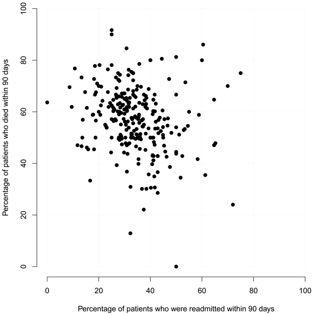
Marginal 90-day readmission and 90-day mortality rates across J = 264 hospitals in California with at least 10 patients aged 65 years or older and diagnosed with pancreatic cancer between 2000–2012. Note, the rates are marginal in the sense that they are not covariate-adjusted.

Finally, we note that there is substantial variation in the patient case-mix across the hospitals. The interquartile range for the percentage nonwhite, for example, is 10.5–35.4%, while the interquartile range for the percentage of patients who are discharged to a hospice, skilled nursing facility or intensive care facility is 24.1–38.9%; see Figures SM-2 and SM-3 in the Supplementary Material A (Haneuse et al. (2022)).

3. Profiling for binary outcomes.

Let $Y_{\mathit{ji}}^{\ast }=0/1$ be a binary indicator of whether or not the ith patient in the jth hospital was readmitted within 90 days of discharge. Note that if a patient died prior to readmission within 90 days, their outcome would be set to $Y_{\mathit{ji}}^{\ast }=0$. An analysis could proceed on the basis of a logistic-Normal GLMM,

$$\text{logit}\mathrm{Pr}(Y_{ji}^{\ast }=1\mid {\mathit{X}}_{ji}^{\ast };{\mathit{\beta }}^{\ast },V_j^{\ast })={\mathit{X}}_{ji}^{\ast T}{\mathit{\beta }}^{\ast }+V_j^{\ast },$$ (1)

where ${\mathit{X}}_{ji}^{\ast }$ is a vector of patient-specific covariates measured prior to discharge and $V_j^{*}$ is a hospital-specific random effect that is taken to arise from a Normal(0, ${\sigma }_v^2$) distribution.

3.1. A measures for performance.

Given model (1), Normand, Glickman and Gatsonis (1997) define the hospital-specific adjusted outcome rate,

$${\mu }_j^a=\frac{1}{n_j}\sum _{i=1}^{n_j}\mathrm{Pr}(Y_{ji}^{\ast }=1\mid {\mathit{X}}_{ji}^{\ast };{\mathit{\beta }}^{\ast },V_j^{\ast }),$$

and the standardized adjusted outcome rate,

$${\mu }^s{}_j=\frac{1}{n_j}\sum _{i=1}^{n_j}\text{E}[\mathrm{Pr}(Y_{ji}^{\ast }=1\mid {\mathit{X}}_{ji}^{\ast };{\mathit{\beta }}^{\ast },V^{\ast })],$$

where the expectation in μ^s_j is with respect to the Normal(0, ${\sigma }_v^2$) distribution for V*. Based on these, the excess readmission ratio is ${\theta }_j={\mu }^a{}_j/{\mu }^s{}_j$. Intuitively, θ_j represents the extent to which the “observed” readmission rate for the jth hospital differs from the “expected” rate for the specific number and case-mix of patients actually treated at the hospital (Normand et al. (2016)). If θ_j > 1.0, one concludes that the rate was higher than would be expected, given the patient case-mix, indicating poor performance. If θ_j < 1.0, one can conclude that the rate was lower than expected, given the patient case-mix, indicating good performance.

Practically, if estimation and inference is to be performed within the frequentist paradigm, then ${\mu }^a{}_j$ can be estimated by plugging in point estimates for $V_j^{\ast }$ and β*. Furthermore, ${\mu }^s{}_j$ can be estimated by approximating the expectation using Gauss–Hermite quadrature, based on estimates of β* and the variance component ${\sigma }_v^{2}1=1$ (Stoer and Bulirsch (2002)). If estimation and inference is to be performed via MCMC within the Bayesian paradigm, then posterior samples of θ_j can be obtained by calculating ${\mu }^a{}_j$ and ${\mu }^s{}_j$ at their current values in the MCMC scheme, again using Gauss–Hermite quadrature for the latter.

3.2. Application to pancreatic cancer data.

Returning to the CMS pancreatic cancer data, we performed a Bayesian analyses for the binary indicator of 90-day readmission and (separately) the binary indicator of 90-day mortality, each based on model (1) with the components of X*: sex, age, race, admission route, Charlson–Deyo comorbidity score (Deyo, Cherkin and Ciol (1992)), length of stay, and discharge location.

The first two columns of Table 1 present posterior medians of the odds ratio parameters from the two logistic-Normal models (i.e., exp{β*}) with boldface highlighting indicating that the corresponding central 95% credible interval excluded 1.0; see Section SM-3 for additional detail. Additionally, Figure 2(a) presents the posterior medians of the excess 90-day readmission ratio, denoted by ${\tilde{\theta }}_{j1}$, and of the excess 90-day mortality ratio, denoted by ${\tilde{\theta }}_{j2}$. Several aspects of the results are worth noting. First, there is substantially greater variation across the hospitals in performance for 90-day mortality (with ${\tilde{\theta }}_{j2}$ varying between 0.40 to 1.63) than in performance for 90-day readmission (${\tilde{\theta }}_{j1}$ 0.76 to 1.19). Second, there is significant discordance in the classification of hospitals are being “good” or “poor” performers for the two outcomes (i.e., whether ${\tilde{\theta }}_{j1}$ or ${\tilde{\theta }}_{j2}$ is less than or greater than 1.0). Specifically, we find that 51 hospitals, represented by red dots, are classified as being poor performers with respect to both readmission and mortality, while 64 hospitals, represented by green dots, are classified as being good performers for both. The black dots indicate hospitals with mixed performance, with the 69 in the top-left quadrant classified as being good performers with respect to readmission but poor performers with respect to mortality and 80 in the bottom-right quadrant classified as being poor performers with respect to readmission but good performers with respect to readmission.

Table 1.

Posterior medians for the odds ratio (OR) parameters from separate logistic-Normal generalized linear mixed models (LN-GLMM) for 90-day readmission and 90-day mortality and for the hazard ratio (HR) parameters from a PEM-MVN hierarchical semicompeting risks model; see Sections 3 and 4.1 for additional detail. Further detail, together with 95% credible intervals (CI), is provided in the Supplementary Material A ((Haneuse et al.) (2022)). Note, estimates highlighted in boldface have 95% CIs that exclude 1.0

	LN-GLMM		PEM-MVN
	Readmission	Death	Readmission prior to death	Death prior to readmission	Death after readmission
	OR	OR	HR	HR	HR
Sex
Male	1.00	1.00	1.00	1.00	1.00
Female	0.90	0.81	0.85	0.80	0.85
Age †	0.86	1.16	0.90	1.10	1.06
Race
White	1.00	1.00	1.00	1.00	1.00
Non-white	1.43	0.94	1.26	0.84	1.06
Admission
Emergency room	1.00	1.00	1.00	1.00	1.00
Other	1.06	1.34	1.15	1.29	1.12
Charlson–Deyo score
≤ 1	1.00	1.00	1.00	1.00	1.00
> 1	1.18	1.39	1.26	1.23	1.23
Length of stay *	1.01	0.86	0.98	0.90	0.89
Discharge location
Home without care	1.00	1.00	1.00	1.00	1.00
Home with care	0.88	1.87	1.06	1.90	1.53
Hospice	0.07	17.6	0.24	10.2	3.21
ICF/SNF	0.63	3.48	1.00	3.50	2.07
Other	0.62	2.35	0.88	2.77	1.39

^†Standardized so that 0 corresponds to an age of 77 years and so that a one unit increment corresponds to 10 years.

^*Standardized so that 0 corresponds to 10 days and so that a one unit increment corresponds to seven days.

Fig. 2.

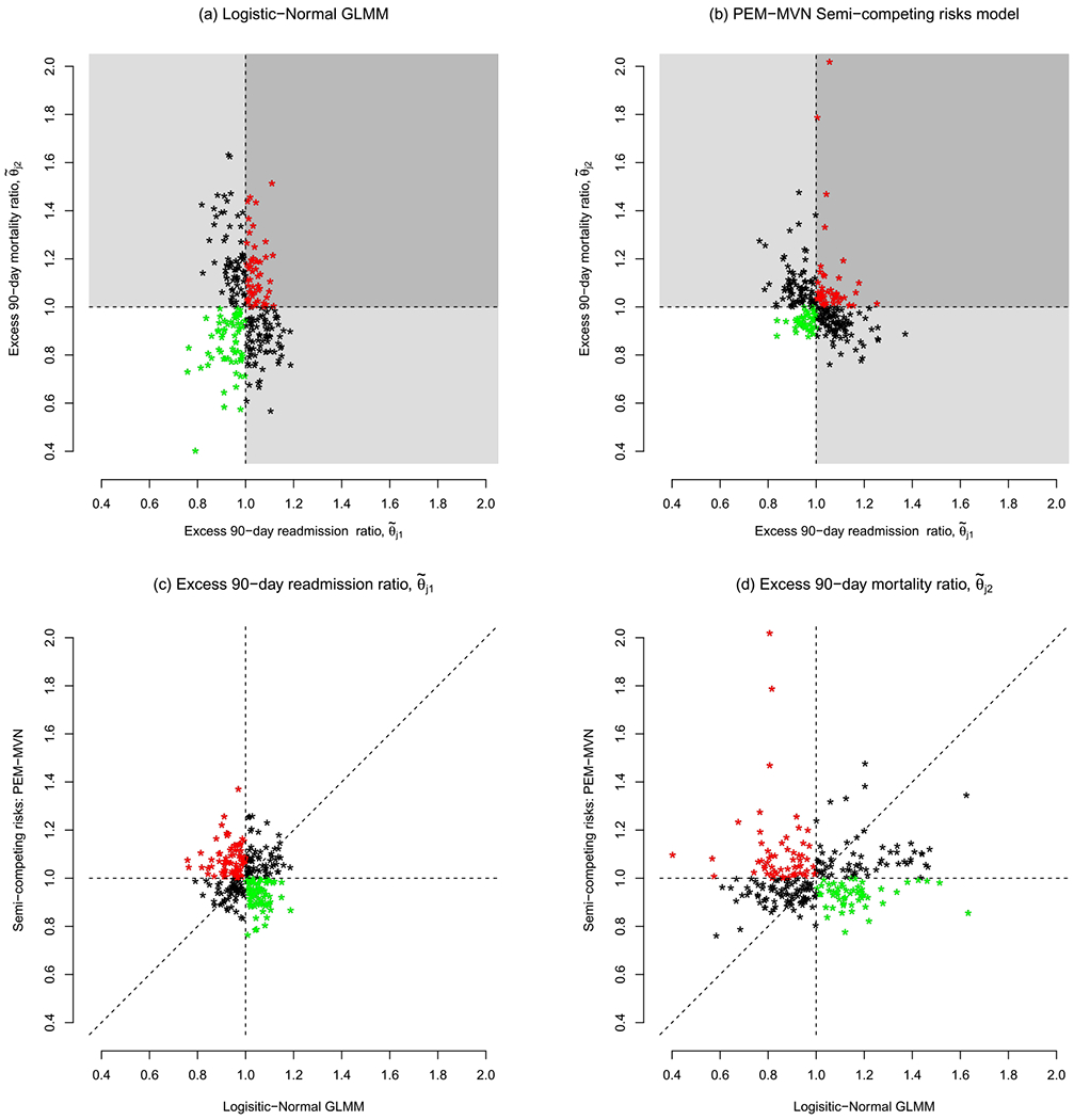
Excess 90-day readmission and 90-day mortality ratios across J = 264 hospitals in California with, at least, 10 patients aged 65 years or older and diagnosed with pancreatic cancer between 2000–2012. Shown in panels (a) and (b) are posterior medians, color coded by whether the value are less than or greater than 1.0: in (a) the results are based on a Bayesian fit of the logistic-Normal GLMM (see Section 3); in (b) the results are based on a PEM-MVN semi-competing risk model (see Sections 4 and 5). In panels (c) and (d), hospitals indicated with green dots were reclassified as having lower-than-expected readmission or mortality by the semicompeting risks analysis (i.e., benefitted), while those indicated with a red dot were reclassified as having higher-than-expected readmission or mortality (i.e. lost).

Together Figures 1 and 2 provide a reasonable basis for questioning the role that performance with respect to 90-day mortality plays when considering performance with respect to 90-day readmission. Specifically, as alluded to in the Introduction, it is plausible that some hospitals are being erroneously classified because mortality is not being explicitly accounted for in either the underlying regression analyses or in the performance metric.

4. Bayesian analyses of cluster-correlated semicompeting risks data.

As will become clear, the metrics and methods proposed in Sections 5 and 6 follow from the fit of a hierarchical model for the cluster-correlated semicompeting risks data. In this section we review a framework for such models proposed by Lee et al. (2016). Throughout, while the methods are applicable to any cluster-correlated semicompeting risks data setting, we use the terms “hospital” and “patient” to be inline with the data application.

4.1. A hierarchical illness-death model.

Let J denote the number of hospitals and n_j the number of patients in the jth hospital, j = 1, …, J. Let T_ji1 and T_ji2 denote the times to readmission and death, respectively, for the ith patient in the jth hospital, for i = 1, …, n_j and j = 1, …, J. In an illness-death model the rates at which a given patient transitions between the initial state (i.e., discharged alive) and the state of experiencing a readmission event and/or the state of experiencing a death event are assumed to be governed by three hazard functions: h₁(t₁), the cause-specific hazard for readmission, given that a mortality event has not occurred; h₂(t₂), the cause-specific hazard for mortality, given that a readmission event has not occurred, and h₃(t₂|t₁), the hazard for mortality, given than a readmission event occurred at time t₁. Toward the analysis of cluster-correlated semicompeting risks data, Lee et al. (2016) proposed the following hierarchical illness-death model:

$$h_1(t_{ji1}\mid {\mathit{X}}_{ji1};{\gamma }_{ji},h_{01},{\mathit{\beta }}_1,V_{j1})={\gamma }_{ji}{h}_{01}(t_{ji1})\exp \{{\mathit{X}}_{ji1}^T{\mathit{\beta }}_1+V_{j1}\},$$ (2)

$$h_2(t_{ji2}\mid {\mathit{X}}_{ji2};{\gamma }_{ji},h_{02},{\mathit{\beta }}_2,V_{j2})={\gamma }_{ji}{h}_{02}(t_{ji2})\exp \{{\mathit{X}}_{ji2}^T{\mathit{\beta }}_2+V_{j2}\},$$ (3)

$$h_3(t_{ji2}\mid t_{ji1},{\mathit{X}}_{ji3};{\gamma }_{ji},h_{03},{\mathit{\beta }}_3,V_{j3})={\gamma }_{ji}{h}_{03}(t_{ji2}\mid t_{ji1})\exp \{{\mathit{X}}_{ji3}^T{\mathit{\beta }}_3+V_{j3}\},$$ (4)

where γ_ji is a patient-specific frailty, X _jig is a vector of transition/patient-specific covariates, β_g is a vector of transition-specific fixed-effect log-hazard ratio regression parameters, and V_j = (V_j1, V_j2, V_j3) is a vector of cluster-specific random effects. For the patient-specific γ_ji frailties, consistent with much of the literature on illness-death models, Lee et al. (2016) proposed that they be assumed to arise from a common Gamma(θ⁻¹, θ⁻¹) distribution such that E[γ_ji] = 1 and V[γ_ji] = θ. For the transition-specific baseline hazard functions, we first note that, because h₀₃(t_ji2|t_ji1) in expression (4) is conditional on the timing of the nonterminal event, analysts are, in principle, faced with the task of specifying its functional form all possible t₁. Practically, this will likely be an onerous task and is typically mitigated via the adoption of a Markov model, such that h₀₃(t_ji2|t_ji1) = h₀₃(t_ji2), or a semi-Markov model, such that h₀₃(t_ji2|t_ji1) = h₀₃(t_ji2 – t_ji1) (e.g., Xu, Kalbfleisch and Tai (2010)). Whichever of these is adopted, Lee et al. (2016) proposed two specifications for the transition-specific baseline hazard functions: (i) that h_0g(t) = α_w,gκ_w,gt^α_w,g−1 so that it corresponds to the hazard of a Weibull(α_w,g, κ_w,g) distribution, and (ii) that h_0g(t) be structured via a piecewise exponentials mixture (PEM) model with the mixing taking place over the number and placement of knots (McKeague and Tighiouart (2000), Haneuse, Rudser and Gillen (2008)). Finally, Lee et al. (2016) proposed two specifications for the distribution of cluster-specific random effects, V_j: (i) a mean-zero multivariate Normal distribution (MVN) with variance-covariance matrix ∑_V, and (ii) a Dirichlet process mixture (DPM) of MVNs (Bush and MacEachern (1996), Ferguson (1973), Walker and Mallick (1997)).

4.2. Bayesian estimation and inference.

To complete the Bayesian specification, prior distributions and corresponding hyperparameters are needed. The exact nature of these depends on various choices made at the first stage of the model specification, including whether parametric Weibull or nonparametric PEM baseline hazard functions are adopted and whether a parametric or nonparametric specification of the distribution for the hospital-specific random effects, V_j, is adopted; see Lee et al. (2016) for a detailed overview.

Given a complete specification of the model, samples from the joint posterior distribution can be obtained via a reversible-jump MCMC algorithm, implemented in the SemiCompRisks package for R, with model comparison based on the deviance information criterion (DIC; Spiegelhalter et al. (2002), Millar (2009)) and/or the log-pseudo marginal likelihood statistic (LPML; Geisser (1993)).

4.3. Application to pancreatic cancer data.

We fit four models to the CMS data, corresponding to combinations of the two baseline hazard specifications (i.e., Weibulls and PEM) and two specifications for the hospital-specific random effects (i.e., MVN and DPM). In each, we adopted semi-Markov specifications for h₀₃(t_ji2|t_ji1) and included the same set of covariates in X as those in X* for the logistic-Normal models in Section 3.2, in each of the three transitions. Comprehensive details, including the choice of hyperparameters, convergence of the MCMC schemes, and posterior summaries are provided in Section SM-4 of the Supplementary Material A (Haneuse et al. (2022)).

Based on the DIC and LMPL model comparison criteria, the model with a PEM specification for the baseline hazard functions and a MVN for the hospital-specific random effects (henceforth labelled as the “PEM-MVN model”) was found to have the best fit (see Table SM-4 in the Supplementary Material A (Haneuse et al. (2022))). The third, fourth and fifth columns of Table 1 present posterior medians for the hazard ratio parameters (i.e., exp{β_g}) for the three transitions with boldface highlighting again indicating that the corresponding central 95% credible interval excluded 1.0.

Comparing the first and third columns, we see that the two analyses indicate different predictor profiles for 90-day readmission. In particular, the semicompeting risks analysis indicates that patients who are admitted via some route other than the ER are at increased risk for 90-day readmisson whereas the standard LN-GLMM analysis indicated no such association. Furthermore, taking mortality into account dramatically changed the profile of associations between discharge location and risk of 90-day readmission.

Comparing the second column to the fourth and fifth, we see that the set of predictors that have 95% credible intervals that exclude 1.0 generally coincide between the two analyses. Furthermore, from the semicompeting risks analysis the associations between a given covariate and death are generally in the same direction whether death is being considered prior to or after a readmission event. The sole exception is for nonwhite race for which there is evidence of a decreased risk of death prior to a readmission event but no evidence of an association with death after a readmission event.

5. Performance metrics for end-of-life care.

Having reframed the investigation of variation in risk of readmission as a problem of semicompeting risks, we propose new metrics for performance for end-of-life care.

5.1. Readmission.

To characterize hospital performance with respect to readmission, we define the cumulative excess readmission ratio for t₁ > 0 as

$${\theta }_{j1}(t_1)=\frac{{\mu }_{j1}^A(t_1)}{{\mu }_{j1}^S(t_1)}$$ (5)

for which the numerator, termed the adjusted cumulative readmission rate, is defined to be

$${\mu }_{j1}^A(t_1)=\frac{1}{n_j}\sum _{i=1}^{n_j}{F}_{ji1}(t_1;V_{j,1},V_{j,2}),$$

where

$$\begin{gathered} F_{ji1}(t_1;V_{j,1},V_{j,2}) \\ ={\int }_0^{t_1}{h}_1(s\mid {\mathit{X}}_{ji1};{\gamma }_{ji},h_{01},{\mathit{\beta }}_1,V_{j1})\exp \left\{-\sum _{g=1}^2{H}_g(s\mid {\mathit{X}}_{jig};{\gamma }_{ji},h_{0g},{\mathit{\beta }}_g,V_{jg})\right\}\partial s, \end{gathered}$$

with $H_g(s|\cdot )={\int }_0^s{h}_g(u|\cdot )\partial u$. Note that F_ji1(t₁; V_j1) is the cumulative incidence function for readmission with death taken as a competing risk (Fine and Gray (1999)). Finally, the denominator in expression (5), termed the standardized adjusted cumulative readmission rate, is defined to be

$${\mu }_{j1}^S(t_1)=\frac{1}{n_j}\sum _{i=1}^{n_j}\text{E}[F_{ji1}(t_1;V_1,V_2)],$$

where the expectation is with respect to the joint distribution of (V₁, V₂).

5.2. Mortality.

To characterize hospital performance with respect to mortality, we define the cumulative excess mortality ratio for t₂ > 0 as

$${\theta }_{j2}(t_2)=\frac{{\mu }_{j2}^A(t_2)}{{\mu }_{j2}^S(t_2)},$$ (6)

for which the numerator, termed the adjusted cumulative mortality rate, is defined to be

$${\mu }_{j2}^A(t_2)=\frac{1}{n_j}\sum _{i=1}^{n_j}{F}_{ji2}(t_2;{\mathit{V}}_j),$$

where F_ji2(t₂; V_j) is the CDF for the marginal distribution of T₂ for the ith individual in the jth hospital induced by the hierarchical illness-death model, given by

$$F_{ji2}(t_2;{\mathit{V}}_j)={\int }_0^{t_2}\left[{\int }_0^s{f}_U(u,s;{\mathit{V}}_j)\partial u+f_{\infty }(s;{\mathit{V}}_j)\right]\partial s,$$ (7)

where f_U(t₁, t₂) is the density for the induced joint distribution on the upper wedge of the support of (T₁, T₂) and f_∞(t₂) is the probability mass corresponding to the timing of the terminal event for patients who experience it prior to the nonterminal event (Frydman and Szarek (2010), Lee et al. (2015), Xu, Kalbfleisch and Tai (2010)). Additional details are given in Section SM-6 of the Supplementary Material A (Haneuse et al. (2022)). Finally, the denominator of expression (6), which we term the standardized adjusted cumulative mortality rate, is defined to be

$${\mu }_{j2}^S(t_2)=\frac{1}{n_j}\sum _{i=1}^{n_j}\text{E}[F_{ji2}(t_2;\mathit{V})],$$

where the expectation is with respect to the joint distribution of V.

5.3. Interpretation and use.

The interpretations of θ_j1(t₁) and θ_j2(t₂) are analogous to that of θ_j described in Section 3. That is, the two metrics can be interpreted as the extent to which the “observed” readmission and mortality rates for jth hospital differ from the corresponding “expected” rates, for the specific number and case mix of patients actually treated at the jth hospital. One key difference, however, is that the proposed measures are defined specifically to be functions of the underlying time scales thus providing additional scope and flexibility in the choice of measure on which to base a decision. Depending on the scientific and/or policy goals of the specific analysis, for example, one might choose a specific time, say (t₁, t₂) = (90, 90) at which to evaluate performance or to consider their trajectories over some fixed time interval, say (0, 90] days.

5.4. Characterization of the posterior distribution of (θ_j1(t₁), θ_j2(t₂)).

The joint posterior distribution of (θ_j1(t₁), θ_j2(t₂)) can be readily-characterized through postprocessing of the samples generated from the MCMC scheme for the underlying hierarchical semi-competing risks model from Section 4. One practical challenge is that the integrals in F_ji1(t₁; V_j,1, V_j,2 and F_ji2(t₂; V _j) as well as the expectations in ${\mu }_{j1}^S(t_1)$ and ${\mu }_{j2}^S(t_2)$ do not have closed-form expressions. They must, therefore, be evaluated numerically (Abramowitz and Stegun (1966), Stoer and Bulirsch (2002)).

For F_ji1(t₁; V_j) and F_ji2(t₂; V_j), we note that the component integrals are defined over finite intervals (i.e., (0, t₁) and (0, t₂), respectively). If the analysis of the hierarchical illness-death model has been conducted using parametric specifications for the baseline hazards (e.g., the Weibull distribution; see Section 4.1) so that F_ji1(t₁; V_j) and F_ji2(t₂; V_j) are smooth functions of time, then one can use Gauss–Legendre quadrature. Considering F_ji2(t₂; V_j), let {(x_k1, w_k1); k₁ = 1, …, K₁)} and {(x_k2, w_k2); k₂ = 1, …, K₂)} be the collections of quadrature points and weights based on the Gauss–Legendre rule with K₁ and K₂ nodes, respectively. These can be obtained, for example, from the gaussquad package in R. Then, for ${\tilde{x}}_{k_1}=x_{k_1}+1$ and ${\tilde{x}}_{k_2}=x_{k_2}+1$, we have the approximation,

$${\widehat{F}}_{ji2}(t_2;{\mathit{V}}_j)=\sum _{k_2=1}^{K_2}\frac{t_2{w}_{k_2}}{2}\left[\left\{\sum _{k_1=1}^{K_1}\frac{t_2{\tilde{x}}_{k_2}{w}_{k_1}}{4}{f}_U\left(\frac{t_2{\tilde{x}}_{k_1}{\tilde{x}}_{k_2}}{4},\frac{t_2{\tilde{x}}_{k_2}}{2};{\mathit{V}}_j\right)\right\}+f_{\infty }\left(\frac{t_2{\tilde{x}}_{k_2}}{2};{\mathit{V}}_j\right)\right].$$

If the analysis has been conducted using the PEM specification, however, our experience has been that Gauss–Legendre quadrature performs poorly. This may be due, in part, to the nonsmooth nature of the induced F_ji1(t₁; V_j,1, V_j,2) and F_ji2(t₂; V_j) at each scan of the MCMC scheme. Since the integration is over a finite interval, however, and the partition of the interval that underpins the PEM model is known at each scan in the MCMC scheme, one can calculate the relevant integrals exactly.

For ${\mu }_{j1}^S(t_1)$ and ${\mu }_{j2}^S(t_2)$, we use Gauss–Hermite quadrature because the integrals within each iteration of the MCMC scheme are with respect to a two- or three-dimensional MVN distribution, respectively, regardless of whether the cluster-specific V_j are taken to arise from a MVN or a Dirichlet process mixture of MVNs (see Section 4.1). Considering, ${\mu }_{j2}^S(t_2)$, let {(x_k3, w_k3); k₃ = 1, …, K₃)}, {(x_k4, w_k4); k₄ = 1, …, K₄)} and {(x_k5, w_k5); k₅ = 1, …, K₅)} be the collections of quadrature points and weights based on the Gauss–Hermite rule with K₃, K₄ and K₅ nodes, respectively. To account for the correlation among the three hospital-specific random effects, we use a Cholesky decomposition (i.e., Σ_V = LL^⊺) to transform the integrand from one involving uncorrelated variates to one involved correlated variates to give the approximation,

$$\widehat{\text{E}}[F_{ji2}(t_2;\mathit{V})]=\sum _{k_3=1}^{K_3}\sum _{k_4=1}^{K_4}\sum _{k_5=1}^{K_5}\frac{t_2{w}_{k_3}{w}_{k_4}{w}_{k_5}}{2{\pi }^{3/2}}{\widehat{F}}_{ji2}\left(t_2;{\mathit{V}}_j^L\right),$$

where ${\mathit{V}}_j^L=(V_{j1}^L,V_{j2}^L,V_{j3}^L)$ with $V_{j1}^L=\sqrt{2}{L}_{11}{x}_{k_3},V_{j2}^L=\sqrt{2}(L_{21}{x}_{k_3}+L_{22}{x}_{k_4})$ and $V_{j3}^L=\sqrt{2}(L_{31}{x}_{k_3}+L_{32}{x}_{k_4}+L_{33}{x}_{k_5})$.

5.5. Practical considerations.

As with all use of numerical integration techniques, analysts will need to contend with a trade-off between accuracy and computational burden. For our use of Gaussian quadrature, the trade-off is dictated by the number of nodes, together with the number of patients in the sample, $N=\sum _{j=1}^J{n}_j$ and the number of samples in the MCMC scheme that will be used to characterize the posterior (denoted here by M). To calculate the denominators in expression (5 across) J = 264 hospitals in the pancreatic cancer data, for example, will require ~4.4×10⁸ calculations if M = 1000 and the number of quadrature nodes is set to five for both V₁ and V₂. To mitigate the corresponding time burden, the implementation in the SemiCompRisks package for R uses compiled C code as the primary computing engine.

To the best of our knowledge, there are no universal rules regarding the degree of accuracy associated with a given number of nodes. Practically, one strategy is to use some common number of nodes, say K, across all instances where a value must be set, and assess the sensitivity of the results as one increases K. When the results become insensitive to increases in K, one can halt the calculations. For the analyses of the pancreatic cancer data presented in the next subsection, we used this strategy with K ∈ {3, 5, 10, 15} and found the greatest relative difference between values based on K = 5 and values based on K = 15, across all calculations of ${\mu }_{j1}^S(\cdot ),{\theta }_{j1}(\cdot ),{\mu }_{j2}^S(\cdot )$, and θ_j2(⋅), to be less an 0.002%. As such, we present results based on K = 5.

5.6. Application to pancreatic cancer data.

Panels (b), (c), and (d) of Figure 2 provide results based on the PEM-MVN model, identified in Section 4.3 as having the best fit to the data; Figures SM-4, SM-5, and SM-6 in the Supplementary Material A (Haneuse et al. (2022)) provide corresponding results for the other three models. Comparing Figure 2(b) with Figure 2(a), we find that overall variation across the J = 264 hospitals in the performance for 90-day readmission is similar under the two analyses with the posterior medians varying from 0.76 to 1.37 under the semicompeting risks analysis compared to 0.76 to 1.19 under the logistic-Normal. Furthermore, although the ranges differ, the variation in the posterior medians for the hospital-specific excess 90-day mortality ratios is also similar, with those under the semicompeting risks analysis varying between 0.76 to 2.02 and those under the logistic-Normal analysis varying between 0.40 to 1.63.

Notwithstanding the comparable overall variation, however, Figures 2(c) and 2(d) indicate that the performance measures for individual hospitals can differ substantially: the percent change in the posterior medians for 90-day readmission (from those based on the logistic-Normal) across the hospitals ranges from −22% to 42%, while the percent change in the posterior medians for 90-day mortality ranges from −48% to 173%. Moreover, the colorcoding in Figure 2(c) indicates that these differences can have potentially profound effects, with 67 hospitals (color-coded in green) that “benefit” from explicit consideration of mortality in that their excess 90-day readmission ratio is less than 1.0 (i.e., lower than expected) under the semicompeting risks analysis whereas it was greater than 1.0 (i.e., higher than expected) under the logistic-Normal analysis. Similarly, there are 77 hospitals that “lose” in the sense that they are classified as being poor performers under the semicompeting risks analysis whereas they were good performance under the logistic-Normal analysis. From Figure 2(d), 55 hospitals that benefit from the semicompeting risks analysis in terms of their performance classification for 90-day mortality while 59 lose.

Finally, while the focus of this case study is on profiling based on outcomes during the 90-day window following discharge, as indicated in Section 5.3, the proposed framework permits consideration of other time windows (in particular, without needing to refit the model) and to consider the evolution of (θ_j1(t₁), θ_j2(t₂)) over time. To these ends, the top two panels of Figure 3 reports results regarding (θ_j1(t₁), θ_j2(t₂)) during six postdischarge windows: 15-, 30-, 45-, 60-, 75-, and 90-days. Interestingly, the values for θ_j1(t₁) are fairly stable over time, while those for θ_j2(t₂) seem to attenuate, with less variability across hospitals in the performance metric evaluated over (0, 90]-days than over, say, (0, 30]-days. This is further clarified in the two lower panels of Figure 3; see Figures SM-7 through SM-11 in the Supplementary Material A (Haneuse et al. (2022)) for additional detail comparing the 90-day window to each of the five shorter ones.

Fig. 3.

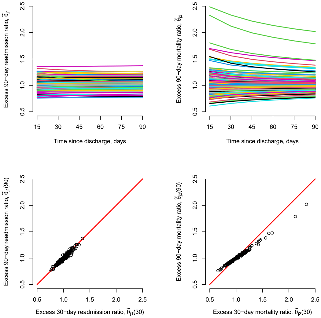
Excess readmission and mortality ratios, evaluated at multiple time windows following discharge, across J = 264 hospitals in California with at least 10 patients aged 65 years or older, and diagnosed with pancreatic cancer between 2000–2012.

6. Profiling.

Following the conduct of a Bayesian analyses, it is typical that summaries of the posterior distribution be reported. For example, the posterior mean or the posterior median is often reported as a point estimate of the corresponding parameter. Additionally, the posterior standard deviation or a 95% credible interval may be reported as a means to communicate uncertainty. In line with this, the results in Figures 1 and 2 regarding excess 90-day readmission and mortality are all based on using the posterior median as a summary for each hospital’s performance measure. The use of the posterior median as a point estimate is intuitive but can also be formally justified as being optimal with respect to L₁ loss. Whether this is a reasonable thing to do depends, however, on whether the L₁ loss is an appropriate loss function for the substantive goal at hand. In this section we consider settings where the substantive goal of the analysis is to profile the performance of the hospitals, possibly toward making some policy decision, such as whether to target a hospital with a quality improvement program or whether and how to adjust their reimbursement rates.

6.1. Loss function-based profiling.

Let θ₁ = (θ₁₁(⋅), …, θ_J1(⋅)) and θ₂ = (θ₁₂(⋅), …, θ_J2(⋅)) denote the collections of J hospital-specific cumulative excess readmission and mortality rates, respectively. We define ${\text{Φ}}_j\equiv {\text{Φ}}_j({\mathit{\theta }}_1,{\mathit{\theta }}_2)$ to be some classification function that corresponds to the profiling goal of interest. For example, following Lin et al. (2009), suppose the profiling goal is establish a framework for identifying the top 100(1 − γ)% of hospitals with respect to their performance on the basis of 90-day readmission so that some action can be taken (e.g., the hospital is rewarded in some way). Addressing this goal could be achieved by ascertaining whether a hospital’s rank is greater than or less than γ(J + 1), for which ${\text{Φ}}_j=I\{\mathrm{rank}({\theta }_{j1}(90))<\gamma (J+1)\}$, where I{⋅} is an indicator function. As a second example, suppose the goal is to identify whether a hospital has higher-/lower-than-expected for 90-day readmission and mortality (i.e., to classify a hospital into one of the four quadrants in the right-hand panel of Figure 1) and then perform some appropriate action. Toward this, a hospital’s classification could be characterized via

$${\text{Φ}}_j=\{\begin{array}{c}1\text{if}{\theta }_{j1}(90)>1.0\text{and}{\theta }_{j2}(90)>1.0,\\ 2\text{if}{\theta }_{j1}(90)>1.0\text{and}{\theta }_{j2}(90)\le 1.0,\\ 3\text{if}{\theta }_{j1}(90)\le 1.0\text{and}{\theta }_{j2}(90)>1.0,\\ 4\text{if}{\theta }_{j1}(90)\le 1.0\text{and}{\theta }_{j2}(90)\le 1.0.\end{array}$$

Since the true θ₁ and θ₂ are unknown, however, the true Φ_j classifications are also unknown and a hospital’s performance must be ascertained on the basis of what we learn from the data. One option for doing this would be to estimate Φ_j by plugging in the posterior medians of the components of θ₁ and θ₂ to give $\tilde{\mathbf{\Phi }}=({\tilde{\mathrm{\Phi }}}_1),\dots ,{\tilde{\mathrm{\Phi }}}_{\mathrm{J}}$. While intuitive, the use of the posterior median is not directly motivated by the profiling goal at hand. Indeed, it is agnostic to the profiling goal and, as such, could be viewed as an arbitrary choice with no better justification than using, say, the posterior mean. To avoid this arbitrariness, one could ascertain the value of Φ_j for a given hospital through consideration of a loss function that is tailored specifically to the profiling goal. Let L(Φ*; Φ⁰) denote such a loss function, with Φ* denoting some candidate value of Φ and Φ⁰ the true value. Intuitively, L(Φ*; Φ⁰) represents the magnitude of the penalty that one is willing to incur as a result of classifying the J hospitals as Φ* when the truth is Φ⁰.

Returning to the goal of identifying the top 100(1 − γ)% hospitals, Lin et al. (2009) consider a number of loss functions that vary in the penalty that is incurred for misclassifying a hospital as being in the 100(1 − γ)% when they are not and/or misclassifying a hospital as not being in the 100(1 − γ)% when they are. One specific option is to assign equal weight (of 1.0) to each such instance of a misclassification (i.e., regardless of the type) to give

$$L({\Phi }^{\ast };{\Phi }^0)=\frac{1}{J}\sum _{j=1}^J\left[\sum _{c\ne c^{\prime }}I\{{\text{Φ}}_j^0=c,{\text{Φ}}_j^{\ast }=c^{\prime }\}\right],$$ (8)

where c and c′ take on values in {0, 1}, which corresponds to the average number of miss-classifications among the J hospitals.

For the second example in which the goal is to categorize hospitals on the basis of whether they have higher-/lower-than-expected rates for 90-day readmission and mortality, one could consider the loss function,

$$L({\Phi }^{\ast };{\Phi }^0)=\frac{1}{J}\sum _{j=1}^J\left(\sum _{c=1}^4\left[\sum _{c^{\prime }=1}^{4}w(c,c^{\prime })I\{{\text{Φ}}_j^0=c,{\text{Φ}}_j^{\ast }=c^{\prime }\}\right]\right),$$ (9)

where w(c, c′) = 0 for c = c′ and w(c, c′) for c ≠ c′ is a penalty that is incurred for classifying a hospital in category c′ when the truth is that they are in category c. Note, when w(c, c′) = 1.0 for all combinations of c′ and c, then expression (9) corresponds to the average number of misclassifications among the J hospitals.

6.2. Estimation.

For a given loss function, an estimate of Φ is obtained by minimizing posterior expected loss or Bayes risk, BR(Φ*) = E_π[L(Φ*; Φ)] with respect to Φ*. Unfortunately, in all but the most trivial settings, BR(Φ*) will not be analytically tractable because it requires integrating over the full joint posterior distribution of the underlying model specification. As such, it will not be possible to write down a closed-form expression for the corresponding minimizer. To resolve this dilemma, we adopt a strategy in which an estimate is obtained by minimizing with respect to Φ* an approximation of the Bayes risk, specifically,

$$\widehat{\text{BR}}({\Phi }^{\ast })=\frac{1}{M}\sum _{m=1}^{M}L({\Phi }^{\ast };{\Phi }^{(m)}),$$

where M is the number of samples retained from the MCMC scheme (i.e., after removing burn-out and thinning) and Φ^(m) is the value of Φ in the mth such sample.

Operationally, this could be achieved postmodel fit (i.e., after all of the MCMC samples have been generated), by: (i) enumerating all possible Φ*, which we denote as 𝒬, (ii) evaluating $\widehat{\mathrm{BR}}({\mathbf{\Phi }}^{\ast })$ for all Φ* ∈ 𝒬, and (iii) selecting the Φ* that corresponds to the smallest $\widehat{\mathrm{BR}}({\mathbf{\Phi }}^{\ast })$. For many profiling settings, however, 𝒬 will be massive so that this brute-force strategy will be computationally prohibitive. To see this, consider the two profiling goals presented so far. For the first of these, if we say that interest lies in identifying the top 10% hospitals for the CA data, then 𝒬 consists of $\left(\begin{array}{c}264\\ 26\end{array}\right)\approx 4.1\times {10}^{35}$ potential classifications. For the second profiling goal of characterizing a hospitals joint performance status with respect to 90-day readmission and 90-day mortality, then 𝒬 consists of 4²⁶⁴ ≈ 8.8 × 10¹⁵⁸ potential classifications.

To resolve this, we propose that researchers adopt one or both of two ad hoc strategies aimed at reducing overall computational burden. The first strategy is a preprocessing step aimed at identifying a subset 𝒬_s ∈ 𝒬 through consideration of $\tilde{\mathbf{\Phi }}$, the value of Φ obtained by plugging in the posterior medians of the components of θ₁ and θ₂. The motivation for doing so is that, although not optimal with respect to the chosen L(Φ*; Φ⁰), $\tilde{\mathbf{\Phi }}$ may be a reasonable basis for ruling out select classifications that are a posteriori unlikely to be optimal. For example, if a hospital ranks as worst on the basis of the J posterior medians of Φ_j = rank(θ_j1(90)) then it may be reasonable to exclude from 𝒬 any classification that places this hospital in the top 10%. Similarly, if a hospital has large values of $\tilde{\theta }{j}_1(90)$ and $\tilde{\theta }{j}_2(90)$ that are both > 1.0, then it may be reasonable to argue that there is little mass in the joint posterior of (θ_j1(90), θ_j2(90)) that supports classifying the hospital in the category where there are lower than expected 90-day rates for both readmission and mortality. Depending on the nature of the approach to ruling out certain classification, the subset 𝒬_s may be substantially smaller than 𝒬, thus rendering a subsequent brute-force search for the classification that yields the minimum $\widehat{\mathrm{BR}}({\mathbf{\Phi }}^{\ast })$ feasible.

The second strategy is a sequential updating algorithm aimed at speeding up the task of finding the minimizer from among the classifications in 𝒬 (or 𝒬_s):

1. Let ${\widehat{\Phi }}^{(l)}=({\widehat{\varphi }}_1^{(l)},{\widehat{\varphi }}_2^{(l)},\dots ,{\widehat{\varphi }}_J^{(l)})$ be the current classification of the J hospitals and $\widehat{\mathrm{BR}}({\mathbf{\Phi }}^{(l)})$ the corresponding approximate Bayes risk.

2. Let 𝒥 be some random reordering of {1, …, J}.

3. Let j* be the first element in 𝒥, and consider all possible options for an update of the classification (i.e.,${\widehat{\varphi }}_{j^{\ast }}^{(l+1)}$). Note, for some loss functions an update for one hospital may require a parallel update to some other hospital. For the loss function, given by expression (8), for example, updating a hospital’s classification as being in the top 10% will require moving one hospital that is currently in the top 10% into the bottom 10%. We propose that such a hospital be chosen at random, possibly with the acknowledgement of any decisions made through the preprocessing strategy that reduced 𝒬 to 𝒬_s.

4. For each classification identified in step (3), compute the approximate Bayes risk based on $({\widehat{\varphi }}_1^{(l)},\dots ,{\widehat{\varphi }}_{j^{\ast }}^{(l+1)},\dots ,{\widehat{\varphi }}_J^{(l)})$. If the minimum of these values is less than the current Bayes risk, then “update” ${\widehat{\varphi }}_{j^{\ast }}^{(l+1)}$ with the corresponding classification.

5. Repeat steps (3) and (4) for all elements in 𝒥.

6. Repeat steps (1)–(5) until no further updates yield smaller values of the approximate Bayes risk (i.e., $\widehat{\text{BR}}({\widehat{\Phi }}^{(l+1)})=\widehat{\text{BR}}({\widehat{\Phi }}^{(l)})$).

We note that, although use of either of the proposed strategies is not accompanied by any guarantee that the optimal classification will be obtained, in our experience use of the random reordering in step (2), together with a range of starting values (including $\tilde{\mathbf{\Phi }}$, invariably led to the same final classification indicating a degree of robustness.

6.3. Application to pancreatic cancer data.

6.3.1. Identification of the top 10% of the hospitals.

Table 2 summarizes the joint classifications of the J = 264 hospitals on the basis of whether they ranked in the top 10% for performance with respect to 90-day readmission and the top 10% for performance with respect to 90-day mortality. Specifically, for each of the four models fit in Section 4.3, the subtables in Table 2 present a classification based on using the posterior median for (θ_j1(90), θ_j2(90)) as well as that based on minimizes the Bayes risk with loss function (8). Inspection of the margins of the four tables indicates that the number of hospitals that end up in one of the four categories is roughly the same whether the classification is based on the posterior medians or via minimization of the Bayes risk. Furthermore, the marginal distributions are relatively robust across the four models. However, the cross-classification between the results based on the posterior median and those based on minimizing the Bayes risk reveals that there is some discordance between the two approaches. Under the PEM-MVN model, for example, seven hospitals that are classified as not being in the top 10% for either outcome when one uses the posterior median are classified as being a top performer for one of them when one minimizes the Bayes risk. Again, however, these observations seem to hold across the four fitted models.

Table 2.

Classification of J = 264 hospitals according to whether they are ranked in the top 10% for 90-day readmission and in the top 10% for 90-day mortality on the basis of: (i) the posterior median for (θ_j1(90), θ_j2(90)) or, (ii) the minimizer of the approximate Bayes risk, $\widehat{\mathrm{BR}}({\mathbf{\Phi }}^{\ast })$, based on the loss function given by expression (8)

		Loss function-based
		No/No	No/Yes	Yes/No	Yes/Yes
WB-MVN
Posterior median	No/No	203	4	3	0	210
	No/Yes	4	23	0	0	27
	Yes/No	3	0	24	0	27
	Yes/Yes	0	0	0	0	0
		210	27	27	0
WB-DPM
Posterior median	No/No	203	3	4	0	210
	No/Yes	3	24	0	0	27
	Yes/No	4	0	23	0	27
	Yes/Yes	0	0	0	0	0
		210	27	27	0
PEM-MVN
Posterior median	No/No	204	3	4	0	211
	No/Yes	3	23	0	0	26
	Yes/No	4	0	22	0	26
	Yes/Yes	0	0	0	1	1
		211	26	26	1
PEM-DPM
Posterior median	No/No	204	3	4	0	211
	No/Yes	3	22	0	0	25
	Yes/No	5	0	21	0	26
	Yes/Yes	0	0	0	1	1
		212	25	25	1

6.3.2. Bivariate classification.

Table 3 summarizes the joint classifications of the J = 264 hospitals on the basis of whether they are found to have higher- or lower-than expected 90-day readmission and 90-day mortality. Specifically, for each of the four models fit in Section 4.3, the subtables in Table 3 present a classification based on using the posterior median for (θ_j1(90), θ_j2(90)) as well as that based on minimizing the Bayes risk with loss function (8).

Table 3.

Classification of J = 264 hospitals according to whether they are found to have higher- or lower-than expected 90-day readmission and 90-day mortality on the basis of: (i) the posterior median for (θ_j1(90), θ_j2(90)) or, (ii) the minimizer of the approximate Bayes risk, $\widehat{\mathrm{BR}}({\mathbf{\Phi }}^{\ast })$, based on the loss function given by expression (9)

		Loss function-based
		Higher/Higher	Higher/Lower	Lower/Higher	Lower/Lower
WB-MVN
Posterior median	Higher/Higher	27	3	4	0	34
	Higher/Lower	0	106	0	0	106
	Lower/Higher	0	0	90	0	90
	Lower/Lower	0	3	4	27	34
		27	112	98	27
WB-DPM
Posterior median	Higher/Higher	20	4	3	0	27
	Higher/Lower	0	112	0	0	112
	Lower/Higher	0	0	84	0	84
	Lower/Lower	0	5	5	31	41
		20	121	92	31
PEM-MVN
Posterior median	Higher/Higher	39	3	2	0	44
	Higher/Lower	0	97	0	0	97
	Lower/Higher	0	0	80	0	80
	Lower/Lower	0	4	2	37	43
		39	104	84	37
PEM-DPM
Posterior median	Higher/Higher	58	4	3	0	65
	Higher/Lower	0	79	0	0	79
	Lower/Higher	1	0	84	0	85
	Lower/Lower	0	6	2	27	35
		59	89	89	27

Focusing on the results based on the PEM-MVN model, we find that six hospitals initially are classified as being good performers for both 90-day readmission and 90-day mortality (i.e., in the “Lower/Lower” category) when the posterior medians are used are reclassified as being poor performers for, at least, one of the outcomes: four are reclassified as being poor performers with respect to 90-day readmission and two with respect to 90-day mortality. Furthermore, five hospitals that are initially classified as being poor performers for both outcomes (i.e., in the “Upper/Upper” category) are classified as being good performers for at least one outcome: three are reclassified as being good performers with respect to 90-day mortality and two with respect to 90-day readmission.

Looking at the loss-function based classifications across the four models, we see that there are some important differences. For example, while 39 hospitals are classified as being poor performers for both 90-day readmission and 90-day mortality under the PEM-MVN model, this number increases to 58 under the PEM-DPM model. Similarly, while 37 hospitals are classified as being good performers for both 90-day readmission and 90-day mortality under the PEM-MVN model, this number decreases to 27 under the PEM-DPM model.

7. Discussion.

The current statistical paradigm for quantifying hospital performance with respect to readmission ignores death as a competing risk. Doing so may, arguably, be reasonable for health conditions with low mortality, although it is unclear what threshold for “low” should be used or even whether a single such threshold exists. Either way, ignoring death as a competing risk is unlikely to be reasonable for monitoring performance corresponding to terminal conditions for which the clinical focus is generally on managing end-of-life quality of care for the patient. For such conditions, given the substantial financial implications involved, quantifying the magnitude of variation and the attributes of hospitals associated with performance on both readmission and mortality in parallel could help to direct and prioritize quality improvement initiatives. This, we argue, represents a fundamental shift away from unidimensional assessments of readmission-based performance for individual health conditions as well as hospital-wide assessments that consider a range of conditions simultaneously (CMS (2021)). Practically, to achieve this we have proposed a novel general framework consisting of four components: (i) a hierarchical model for the underlying semicompeting risks data, (ii) two novel measures of performance, (iii) a loss-function based approach to classifying the performance of a collection of hospitals, and (iv) a series of pragmatic strategies for mitigating computational burden. While the first of these was described and evaluated via simulation in Lee et al. (2016), components (ii)–(iv) are the key contributions of this paper.

The proposed framework is motivating by an on-going collaboration regarding end-of-life care for patients with a terminal cancer diagnosis. Within this backdrop, this paper presents key methodologic issues and the proposed framework via a detailed case-study using data on N = 17,685 patients diagnosed with pancreatic cancer at one of J = 264 hospitals in California between 2000–2012. Several interesting aspects of the case study deserve additional discussion. First, from a substantive perspective, the results show that the classification of a given hospital may change when one grounds the evaluation of performance within the semi-competing risks framework in lieu of using the output from a logistic-Normal GLMM and when one uses a loss-function based approach to classifying hospitals in lieu of using the posterior median as a plug-in estimator. In considering the differences between the results based on a logistic-Normal model and those based on a hierarchical model for semicompeting risks (see Figures 2(c) and 2(d)), additional analyses reveal that hospital volume seemed to play little-to-no systematic role in dictating whether a hospitals was reclassified on the basis of readmission. However, mortality prior to readmission did appear to play a meaningful role. Specifically, in regard to the loss function given by expression (8) we found that hospitals with (relatively) low or high mortality prior to readmission were more likely to be classified as “winners” (i.e., they benefitted from the use of the semicompeting risks analysis). Furthermore, in regard to the loss function given by expression (9) we found that the rate at which hospitals were differentially being reclassified as winners (i.e., being reclassified into the “lower-than-expected” group) increased with the mortality rate prior to readmission. Whether these observations/insight are generalizable to all settings is unclear, however; whether differences manifest is likely a function of many aspects of the data (e.g., the patient and hospital characteristics) and underlying covariation in the outcomes.

A second interesting aspect of the case study is the sensitivity of the classifications across the four model specifications in Table 3. In considering the relatively complex nature of cluster-correlated semicompeting risks data, that this is the case should not, we believe, be unexpected. Indeed, given that the PEM specification for the baseline hazards is substantially more flexible than the Weibull specification and, similarly, that the DPM specification for the hospital-specific random effects is substantially more flexible than the MVN, it would be surprising if there was no variability in the results across the specifications. Moreover, even in the more standard binary outcome setting, the use of a MVN for the random effects vs. a DPM will likely result in differences in the final fit (Antonelli, Trippa and Haneuse (2016)) and, hence, the final classification(s). Indeed, this is a phenomenon that likely affects all statistical analysis of real data that involve complex, hierarchical structure. Of course, in practice, one never knows the “truth” so that the use of established and understood model fit criteria, such the DIC and/or LMPL measures referenced in Section 4.2, are critical tools, specifically, as a means to choosing the final model before seeing the final profiling results.

Finally, the results in Figure 3, together with those in Figures SM-7 through SM-11 of the Supplementary Material A (Haneuse et al. (2022)), serve to highlight the policy opportunities associated with embedding the task at hand within a hierarchical semicompeting risks model. Specifically, that the model explicitly considers and borrows across time provides a framing for informing policy interventions that are tailored to, for example, improving performance in the immediate aftermath following discharge without affecting longer-term performance. In considering this, it is important to note that the trajectories in Figure 3 may be (generally) parallel, in part at least, because of the sole inclusion of random intercepts in models (2)–(4). One way to enhance this model would be to additionally include random slopes for time, although the interpretation of what these components capture would need to be carefully considered in the profiling context of this paper. Finally, in considering whether and how current federal programs may be expanded to include end-of-life conditions, such as pancreatic cancer, results such as those presenting in Figure 3 may serve as important information in selecting an appropriate window.

We note that the proposed framework enjoys a number of appealing features, including that the underlying hierarchical model need only be fit once and that analysts are free to select their own loss functions, as appropriate to the context. It is also important to note, however, that the complexity of task and the size of most datasets that will inform profiling efforts result in numerous practical challenges. Two of these we directly address in this paper: Section 5.5 considers strategies for mitigating computational issues related to calculating integrals inherent to the calculation the components of θ_j1(t₁) and θ_j2(t₂), while Section 6.2 presents efficient strategies for finding the minimizer of $\widehat{\mathrm{BR}}({\mathbf{\Phi }}^{\ast })$. Beyond these, although not the focus of this paper, fitting the hierarchical illness-death model requires care, especially when the event rates are low and/or the follow-up window is short. In such information-sparse settings, however, the options to specify key components of the model to be parametric (i.e., the baseline hazards and the distribution of V_j) will provide a way forward. Additionally, that implementation of the methods in the SemiCompRisks package for R involves the use of compiled C code provides substantial computational efficiency (Alvares et al. (2019))

Building on the work proposed here, there are many avenues for further work. First, we note that the specific profiling context that motivated this work is that of how federal agencies in the United States incentivize quality improvement in relation to all-cause readmission, in particular, through the Hospital Inpatient Quality Improvement Program and the Hospital Readmissions Reduction Program. Outside of this context, the identification of “unusual” health-care providers is also an important policy goal, one for which an assessment of whether a performance metric, such as θ_j1(t₁) or θ_j2(t₂), lies above or below some threshold (e.g., 1.0) is arguably inappropriate (Jones and Spiegelhalter (2011)). Moreover, extending methods geared toward this goal, such as the funnel plots of Spiegelhalter (2005), to jointly consider readmission and mortality is an important avenue for future work. A second avenue is to consider strategies for specifying the weights in expression (9). While the inclusion of the weights provides a more general loss function and keeps the proposed work inline with prior work on loss functions for hospital profiling (e.g., Lin et al. (2006)), the data application as presented does not consider different weighting schemes. This is, in part, because specifying a weighting scheme that corresponds to a reasonable strategy for penalizing “mistakes” is a task that will typically involve deliberations between analysts, subject-matter experts, and policymakers. How to best do this will likely be context specific, but it seems plausible that general guidelines could be developed to help in the process. Third, we note that the data application focuses on the first readmission following a diagnosis of pancreatic cancer. While some patients will eventually experience more than one readmission event, focusing exclusively on the first enables a consistent framing of the clinical scenario that is being considered (and hence what is meant by “quality”). Moreover, simultaneous consideration of multiple hospitalization would, we believe, result in a mixing of clinical scenarios for which decisions are likely to be very different. Nevertheless, methodologically, it is of interest to consider how one would incorporate multiple hospitalizations (e.g., Mazroui et al. (2012)). Finally, a critical policy consideration is how the proposed methods could be incorporated into existing federal quality improvement programs. To that end, key considerations will include the incidence of the condition at hand as well as the window over which “quality” is assessed. For the context that motivated this work, pancreatic cancer is relatively rare (especially relative to a condition such as heart failure) which, in turn, required consideration of a relatively large window of 13 years (see Section 2). While specific decisions will likely be condition-specific, how one would specify an appropriate window will likely consultation with subject-matter experts and policymakers. Fourth, our approach has important implications for policymakers and researchers when assessing hospital quality. Metrics ignoring both the competing risk of mortality and within-hospital correlation of patient outcomes may misclassify hospitals both due to the risk of mortality and to overstating the certainty for hospital-based inferences. All-cause readmission metrics, for instance, combine disease-based and procedure-based cohorts where the force of mortality varies widely across the cohorts. We focused on the latter in this manuscript and encourage measure developers to take a closer look at this issue.

Finally, in considering the role that mortality plays as a competing risk, we have adopted an overarching approach to hospital performance that mirrors the GLMM-based approach, originally proposed by Normand, Glickman and Gatsonis (1997), for univariate binary outcomes. For the latter, a number of recent papers have examined various aspects of this approach, including: advocating for the use of direct standardization to some common population (i.e., instead of standardization to the patients actually seen at the hospital) (George et al. (2017), Varewyck et al. (2014)), comparing the use of fixed vs. random effects (Chen et al. (2021), Kalbfleisch and Wolfe (2013), Varewyck et al. (2014)), investigating the impact of measurement error regarding case-mix adjustment variables (Şentürk et al. (2020)), and examining whether and how hospital-level characteristics should be included as part of the model specification (George et al. (2017), He et al. (2013), Silber et al. (2010)). Furthermore, motivated by challenges faced in the profiling of dialysis centers, a number of recent papers have sought to extend existing methods in new directions, including time-dynamic profiling of, say, 30-day readmission over the course of some follow-up period (Estes et al. (2018)) and new models for profiling adverse recurrent events (Estes et al. (2020)). All of these are complex and interesting issues that need careful consideration of the end-of-life profiling context as well as the potential implications of ignoring mortality as a competing risks for other metrics that are commonly used, such as the Healthcare Effectiveness Data and Information Set (HEDIS) performance measures. We do note, however, that, in mirroring the approach of Normand, Glickman and Gatsonis (1997), the proposed methods are aligned with the philosophy that underpins the Hospital Inpatient Quality Improvement Program and the Hospital Readmissions Reduction Program as they are currently run. In that sense the methods we propose could, in principle, be implemented immediately and provide a means to enhancing quality of end-of-life care.

Supplementary Material

Supplementary Material

Section SM-1: Table summarizing patient characteristics and outcomes

Section SM-2: Exploratory data analyses for the CMS pancreatic cancer data

Section SM-3: Details and results from fits of logistic-Normal generalized linear mixed models for the binary outcomes of 90-day readmission and 90-day mortality

Section SM-4: Details and results from the fit of four hierarchical semicompeting risks models to the CMS pancreatic cancer data

Section SM-5: Additional results regarding the performance metrics for the CMS pancreatic cancer data

Section SM-6: Additional technical details regarding F_ji2(t₂; V_j)

REFERENCES

- Abramowitz M. and Stegun IA, eds. (1966). Handbook of Mathematical Functions, with Formulas, Graphs, and Mathematical Tables 55. Dover, New York. MR0208797 [Google Scholar]
- Alvares D, Haneuse S, Lee C and Lee KH (2019). SemiCompRisks: An R package for the analysis of independent and cluster-correlated semi-competing risks data. R J. 11 376. [DOI] [PMC free article] [PubMed] [Google Scholar]
- Antonelli J, Trippa L and Haneuse S (2016). Mitigating bias in generalized linear mixed models: The case for Bayesian nonparametrics. Statist. Sci 31 80–95. MR3458594 https://doi.org/10.1214/15-STS533 [DOI] [PMC free article] [PubMed] [Google Scholar]
- Bates J, Lewis S and Pickard A (2019). Education Policy, Practice and the Professional. Bloomsbury Publishing. [Google Scholar]
- Bush CA and MacEachern SN (1996). A semiparametric Bayesian model for randomised block designs. Biometrika 83 275–285. [Google Scholar]
- Chen Y, Şentürk D, Estes JP, Campos LF, Rhee CM, Dalrymple LS, Kalantar-Zadeh K and Nguyen DV (2021). Performance characteristics of profiling methods and the impact of inadequate case-mix adjustment. Comm. Statist. Simulation Comput 50 1854–1871. MR4280725 https://doi.org/10.1080/03610918.2019.1595649 [DOI] [PMC free article] [PubMed] [Google Scholar]
- CMS (2021). Hospital-Wide All-Cause, Unplanned Readmission Measure (HWR). Available at https://cmit.cms.gov/CMIT_public/ReportMeasure?measureRevisionId=15918. Accessed: 13th July, 2021.
- Daniels MJ andNormand S-LT (2005). Longitudinal profiling of health care units based on continuous and discrete patient outcomes. Biostatistics 7 1–15. [DOI] [PMC free article] [PubMed] [Google Scholar]
- Deyo RA, Cherkin DC and Ciol MA (1992). Adapting a clinical comorbidity index for use with ICD-9-CM administrative databases. J. Clin. Epidemiol 45 613–619. [DOI] [PubMed] [Google Scholar]
- Estes JP, Nguyen DV, Chen Y, Dalrymple LS, Rhee CM, Kalantar-Zadeh K and ŞentÜrk D (2018). Time-dynamic profiling with application to hospital readmission among patients on dialysis. Biometrics 74 1383–1394. MR3908156 https://doi.org/10.1111/biom.12908 [DOI] [PMC free article] [PubMed] [Google Scholar]
- Estes JP, Chen Y, SentÜrk D, Rhee CM, KÜrÜm E, You AS, Streja E, Kalantar-Zadeh K and Nguyen DV (2020). Profiling dialysis facilities for adverse recurrent events. Stat. Med 39 1374–1389. [DOI] [PMC free article] [PubMed] [Google Scholar]
- Ferguson TS (1973). A Bayesian analysis of some nonparametric problems. Ann. Statist 1 209–230. MR0350949 [Google Scholar]
- Fine JP and Gray RJ (1999). A proportional hazards model for the subdistribution of a competing risk. J. Amer. Statist. Assoc 94 496–509. MR1702320 https://doi.org/10.2307/2670170 [Google Scholar]
- Friebel R, Hauck K, Aylin P and Steventon A (2018). National trends in emergency readmission rates: A longitudinal analysis of administrative data for England between 2006 and 2016. BMJ Open 8 e020325. 10.1136/bmjopen-2017-020325 [DOI] [PMC free article] [PubMed] [Google Scholar]
- Frydman H and Szarek M (2010). Estimation of overall survival in an ‘illness-death’ model with application to the vertical transmission of HIV-1. Stat. Med 29 2045–2054. MR2758446 https://doi.org/10.1002/sim.3949 [DOI] [PubMed] [Google Scholar]
- Geisser S (1993). Predictive Inference. Monographs on Statistics and Applied Probability 55. CRC Press, New York. MR1252174 https://doi.org/10.1007/978-1-4899-4467-2 [Google Scholar]
- George EI, RoČkovÁ V, Rosenbaum PR, Satopää VA and Silber JH (2017). Mortality rate estimation and standardization for public reporting: Medicare’s Hospital Compare. J. Amer. Statist. Assoc 112 933–947. MR3735351 https://doi.org/10.1080/01621459.2016.1276021 [Google Scholar]
- Goldstein H and Spiegelhalter DJ (1996). League tables and their limitations: Statistical issues in comparisons of institutional performance. J. R. Stat. Soc., A 159 385–409. [Google Scholar]
- Haneuse S, Rudser KD and Gillen DL (2008). The separation of timescales in Bayesian survival modeling of the time-varying effect of a time-dependent exposure. Biostatistics 9 400–410. [DOI] [PubMed] [Google Scholar]
- Haneuse S, Dominici F, Normand S-L and Schrag D (2018). Assessment of between-hospital variation in readmission and mortality after cancer surgical procedures. JAMA Network Open 1 e183038–e183038. [DOI] [PMC free article] [PubMed] [Google Scholar]
- Haneuse S, Schrag D, Dominici F, Normand S-L and Lee KH (2022). Supplement to “Measuring performance for end-of-life care.” 10.1214/21-AOAS1558SUPPA, [DOI] [PMC free article] [PubMed] [Google Scholar]
- Hatfield LA, Baugh CM, Azzone V and Normand S-LT (2017). Regulator loss functions and hierarchical modeling for safety decision making. Med. Decis. Mak 37 512–522. [DOI] [PMC free article] [PubMed] [Google Scholar]
- He K, Kalbfleisch JD, Li Y and Li Y (2013). Evaluating hospital readmission rates in dialysis facilities; adjusting for hospital effects. Lifetime Data Anal. 19 490–512. MR3119994 https://doi.org/10.1007/s10985-013-9264-6 [DOI] [PubMed] [Google Scholar]
- Jones HE and Spiegelhalter DJ (2011). The identification of “unusual” health-care providers from a hierarchical model. Amer. Statist 65 154–163. MR2848190 https://doi.org/10.1198/tast.2011.10190 [Google Scholar]
- Kalbfleisch J and Wolfe R (2013). On monitoring outcomes of medical providers. Stat. Biosci 5 286–302. [Google Scholar]
- Kristensen SR, Bech M and Quentin W (2015). A roadmap for comparing readmission policies with application to Denmark, England, Germany and the United States. Health Policy 119 264–273. [DOI] [PubMed] [Google Scholar]
- Laird N and Louis T (1989). Empirical Bayes ranking methods. Journal of Educational Statistics 14 29–46. [Google Scholar]
- Landrum MB, Normand S-LT and Rosenheck RA (2003). Selection of related multivariate means: Monitoring psychiatric care in the Department of Veterans Affairs. J. Amer. Statist. Assoc 98 7–16. MR1977196 https://doi.org/10.1198/016214503388619049 [Google Scholar]
- Leckie G and Goldstein H (2009). The limitations of using school league tables to inform school choice. J. Roy. Statist. Soc. Ser. A 172 835–851. MR2751830 https://doi.org/10.1111/j.1467-985X.2009.00597.x [Google Scholar]
- Lee KH, Haneuse S, schrag D and Dominici F (2015). Bayesian semiparametric analysis of semi-competing risks data: Investigating hospital readmission after a pancreatic cancer diagnosis. J. R. Stat. Soc. Ser. C. Appl. Stat 64 253–273. MR3302299 https://doi.org/10.1111/rssc.12078 [DOI] [PMC free article] [PubMed] [Google Scholar]
- Lee KH, Dominici F, schrag D and Haneuse S (2016). Hierarchical models for semicompeting risks data with application to quality of end-of-life care for pancreatic cancer. J. Amer. Statist. Assoc 111 1075–1095. MR3561930 https://doi.org/10.1080/01621459.2016.1164052 [DOI] [PMC free article] [PubMed] [Google Scholar]
- Lin R, Louis TA, Paddock SM and Ridgeway G (2006). Loss function based ranking in two-stage, hierarchical models. Bayesian Anal. 1 915–946. MR2282211 https://doi.org/10.1214/06-BA130 [DOI] [PMC free article] [PubMed] [Google Scholar]
- Lin R, Louis TA, Paddock SM and Ridgeway G (2009). Ranking USRDS provider specific SMRs from 1998-2001. Health Serv. Outcomes Res. Methodol 9 22–38. 10.1007/s10742-008-0040-0 [DOI] [PMC free article] [PubMed] [Google Scholar]
- Mazroui Y, Mathoulin-Pelissier S, Soubeyran P and Rondeau V (2012). General joint frailty model for recurrent event data with a dependent terminal event: Application to follicular lymphoma data. Stat. Med 31 1162–1176. MR2925687 https://doi.org/10.1002/sim.4479 [DOI] [PubMed] [Google Scholar]
- McKeague IW and Tighiouart M (2000). Bayesian estimators for conditional hazard functions. Biometrics 56 1007–1015. MR1815579 https://doi.org/10.1111/j.0006-341X.2000.01007.x [DOI] [PubMed] [Google Scholar]
- Millar RB (2009). Comparison of hierarchical Bayesian models for overdispersed count data using DIC and Bayes’ factors. Biometrics 65 962–969. MR2649870 https://doi.org/10.1111/j.1541-0420.2008.01162.x [DOI] [PubMed] [Google Scholar]
- NHS NSS (2019). Hospital Scorecard. Available at https://www.isdscotland.org/Health-Topics/Quality-Indicators/Hospital-Scorecard/. Accessed: 14th April, 2014.
- Normand S-LT, Glickman ME and Gatsonis CA (1997). Statistical methods for profiling providers of medical care: Issues and applications. J. Amer. Statist. Assoc 92 803–814. [Google Scholar]
- Normand S-LT, Ash AS, Fienberg SE, Stukel TA, Utts J and Louis TA (2016). League tables for hospital comparisons. Annu. Rev. Stat. Appl 3 21–50. [Google Scholar]
- Ohlssen DI, Sharples LD and Spiegelhalter DJ (2007). Flexible random-effects models using Bayesian semi-parametric models: Applications to institutional comparisons. Stat. Med 26 2088–2112. MR2364293 https://doi.org/10.1002/sim.2666 [DOI] [PubMed] [Google Scholar]
- Paddock SM (2014). Statistical Benchmarks for Health Care Provider Performance Assessment: A Comparison of Standard Approaches to a Hierarchical Bayesian Histogram-Based Method. Health Serv. Res 49 1056–1073. [DOI] [PMC free article] [PubMed] [Google Scholar]
- Paddock SM and Louis TA (2011). Percentile-based empirical distribution function estimates for performance evaluation of healthcare providers. J. R. Stat. Soc. Ser. C. Appl. Stat 60 575–589. MR2829191 https://doi.org/10.1111/j.1467-9876.2010.00760.x [DOI] [PMC free article] [PubMed] [Google Scholar]
- Paddock SM, Ridgeway G, Lin R and Louis TA (2006). Flexible distributions of triplegoal estimates in two-stage hierarchical models. Comput. Statist. Data Anal 50 3243–3262. MR2239666 https://doi.org/10.1016/j.csda.2005.05.008 [DOI] [PMC free article] [PubMed] [Google Scholar]
- Ridgeway G, Nørgaard M, Rasmussen TB, Finkle WD, Pedersen L, Bøtker HE and Sørensen HT (2019). Benchmarking Danish hospitals on mortality and readmission rates after cardiovascular admission. Clin. Epidemiol 11 67. [DOI] [PMC free article] [PubMed] [Google Scholar]
- Robinson JW, Zeger SL and Forrest CB (2006). A hierarchical multivariate two-part model for profiling providers’ effects on health care charges. J. Amer. Statist. Assoc 101 911–923. MR2324092 https://doi.org/10.1198/016214506000000104 [Google Scholar]
- Samsky MD, Ambrosy AP, Youngson E, Liang L, Kaul P, Hernandez AF, Peterson ED and McAlister FA (2019). Trends in readmissions and length of stay for patients hospitalized with heart failure in Canada and the United States. JAMA Cardiol 4 444–453. 10.1001/jamacardio.2019.0766 [DOI] [PMC free article] [PubMed] [Google Scholar]
- Şentürk D, Chen Y, Estes JP, Campos LF, Rhee CM, Kalantar-Zadeh K and Nguyen DV (2020). Impact of case-mix measurement error on estimation and inference in profiling of health care providers. Comm. Statist. Simulation Comput 49 2206–2224. MR4143441 https://doi.org/10.1080/03610918.2018.1515360 [DOI] [PMC free article] [PubMed] [Google Scholar]
- Shen W and Louis TA (1998). Triple-goal estimates in two-stage hierarchical models. J. R. Stat. Soc. Ser. B. Stat. Methodol 60 455–471. MR1616061 https://doi.org/10.1111/1467-9868.00135 [Google Scholar]
- Silber JH, Rosenbaum PR, Brachet TJ, Ross RN, Bressler LJ, Even-Shoshan O, Lorch SA and Volpp KG (2010). The hospital compare mortality model and the volume–outcome relationship. Health Serv. Res 45 1148–1167. [DOI] [PMC free article] [PubMed] [Google Scholar]
- Spiegelhalter DJ (2005). Funnel plots for comparing institutional performance. Stat. Med 24 1185–1202. MR2134573 https://doi.org/10.1002/sim.1970 [DOI] [PubMed] [Google Scholar]
- Spiegelhalter DJ, Best NG, Carlin BP and Van der Linde A (2002). Bayesian measures of model complexity and fit. J. R. Stat. Soc. Ser. B. Stat. Methodol 64 583–639. MR1979380 https://doi.org/10.1111/1467-9868.00353 [Google Scholar]
- Stoer J and Bulirsch R (2002). Introduction to Numerical Analysis, 3rd ed. Texts in Applied Mathematics 12. Springer, New York. MR1923481 https://doi.org/10.1007/978-0-387-21738-3 [Google Scholar]
- Varewyck M, Goetghebeur E, Eriksson M and Vansteelandt S (2014). On shrinkage and model extrapolation in the evaluation of clinical center performance. Biostatistics 15 651–664. [DOI] [PMC free article] [PubMed] [Google Scholar]
- Walker SG and Mallick BK (1997). Hierarchical generalized linear models and frailty models with Bayesian nonparametric mixing. J. Roy. Statist. Soc. Ser. B 59 845–860. MR1483219 https://doi.org/10.1111/1467-9868.00101 [Google Scholar]
- Westert GP, Lagoe RJ, Keskimäki I, Leyland A and Murphy M (2002). An international study of hospital readmissions and related utilization in Europe and the USA. Health Policy 61 269–278. [DOI] [PubMed] [Google Scholar]
- Xu J, Kalbfleisch JD and Tai B (2010). Statistical analysis of illness-death processes and semicompeting risks data. Biometrics 66 716–725. MR2758207 https://doi.org/10.1111/j.1541-0420.2009.01340.x [DOI] [PubMed] [Google Scholar]
Associated Data
This section collects any data citations, data availability statements, or supplementary materials included in this article.
Supplementary Materials