

SUMMARY
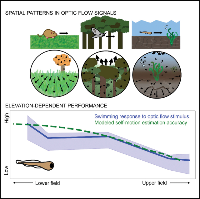
Animals benefit from knowing if and how they are moving. Across the animal kingdom, sensory information in the form of optic flow over the visual field is used to estimate self-motion. However, different species exhibit strong spatial biases in how they use optic flow. Here, we show computationally that noisy natural environments favor visual systems that extract spatially biased samples of optic flow when estimating self-motion. The performance associated with these biases, however, depends on interactions between the environment and the animal’s brain and behavior. Using the larval zebrafish as a model, we recorded natural optic flow associated with swimming trajectories in the animal’s habitat with an omnidirectional camera mounted on a mechanical arm. An analysis of these flow fields suggests that lateral regions of the lower visual field are most informative about swimming speed. This pattern is consistent with the recent findings that zebrafish optomotor responses are preferentially driven by optic flow in the lateral lower visual field, which we extend with behavioral results from a high-resolution spherical arena. Spatial biases in optic-flow sampling are likely pervasive because they are an effective strategy for determining self-motion in noisy natural environments.
In brief
Alexander et al. model natural motion statistics, neural responses, and behavior to show the benefit of spatial biases for self-motion estimation from optic flow, both in general and for the larval zebrafish. Their analysis combines a framework for self-motion estimation in noisy environments with a dataset of optic flow in zebrafish habitats.
Graphical Abstract
INTRODUCTION
Information about self-motion is potentially available from many sources. Inertia-based signals can be measured by vestibular systems, proprioception provides feedback on the forces generated by motor systems, and even haptic information is available, for example, from the wind in our hair. Among the diverse sensing modalities for self-motion, vision stands out as a key source of information for self-motion estimation across the animal kingdom. Visual cues to self-motion are well characterized by optic flow: the movement of features or brightness gradients across the visual field over time.
Laboratory experiments have shown that visual stimuli simulating optic flow during self-motion prompt robust behavioral responses in an impressive array of animals. The responses of flying insects to optic flow are well studied, from flies and bees to dragonflies and locusts.1 For example, bees have been shown to use optic flow to measure distance, maintain flight speed, control landings, and detect objects.2–4 Birds are likewise responsive to optic flow5: for example, parakeets navigate corridors by balancing lateral optic flow,6 and seagulls use optic flow to set their hovering height.7 Optic flow is not just important for animals that fly. Humans can use optic flow cues to predict collisions,8 estimate direction and distance of travel,9,10 maintain upright posture,11,12 and walk toward targets.13–15 In rodents, optic flow has been shown to affect representations of heading direction16 and to be combined with proprioceptive information during locomotion.17
In aquatic environments, optic flow is an important cue for self-motion estimation during swimming and self-stabilization against water currents.18 Like terrestrial vertebrates, different species of fish move both their eyes and their bodies in response to optic-flow cues.19–22 The larval zebrafish, Danio rerio, is of particular interest in this domain due to its use as a model organism in neuroscience for a broad set of behaviors and neural systems. Their tendency to swim along with moving visual stimuli is called the optomotor response (OMR). This behavior likely allows these fish to self-stabilize in moving currents in the wild; for example, as they swim forward in response to forward drifting stimuli, they stay “in place” visually. The amenability of larval zebrafish to whole-brain functional imaging, combined with the OMR behavior, has supported advances in understanding the circuitry that drives optic flow processing in the vertebrate brain.23,24
Although self-motion can in principle produce useful optic flow cues across the entire visual field,25,26 many animals appear to give priority to motion cues in a subset of their visual field. For example, different species of moths prefer to look either up or down to guide their behaviors,27,28 wasps maintain a specific visual angle above their nests during homing flights,29 praying mantises respond preferentially to optic flow in the central visual field,30 and humans prioritize the lower visual field to maintain posture.31 In flies, the lower field is preferred for course correction,32 and lower and upper fields are used for translation and rotation estimation, respectively.33 It was recently shown that the zebrafish OMR is driven preferentially by visual motion in regions of the lower visual field on the left and right sides of the animal.34
Optimal coding models of sensory processing predict that these spatial biases should vary lawfully in response to the statistics of the motion cues available in the visual experience or evolutionary context of each animal.35,36 Indeed, optic flow fields generated from natural environments can be sparse and noisy, putting pressure on animals to sample the most informative spatial regions. Different ecological niches likely correspond to systematic differences in spatial patterns in the availability of optic-flow cues. Previous work has used geometric models and measurements from videos to examine how natural experience may shape spatial biases in the fly26,37 and hawkmoth27 for estimating self-motion. However, given the complexity of self-motion-generated optic flow during natural behavior, the hypothesis that spatial biases are adaptive has proven challenging to test, both in general and for any specific model organism. Modeling the relationship between optic flow signals and self-motion estimates requires a combined consideration of environment geometry, signal and noise strength, motion-limiting behaviors, and neuronal receptive field structure.
We begin with an exploration of the general problem of visual self-motion estimation in natural environments. We model self-motion estimation from samples of naturalistic optic flow fields, demonstrating the effects of a set of pertinent environmental, behavioral, and neural factors. We show that a wide variety of error patterns are generated by different settings for each of these factors, suggesting that a holistic understanding of an animal’s habitat, actions, and receptive field structure is required to determine an advantageous spatial bias. We then model each of these factors for the visual experience of a specific model organism, the larval zebrafish, using omnidirectional videos captured in their native habitats during calibrated self-motion trajectories controlled by a custom-built robotic arm. Our results suggest that these animals can most reliably estimate their forward self-motion from regions in the lateral lower visual field, which is consistent with prior behavioral measures.34 Using a spherical stimulation arena covering more than 90% of the visual surround,38 we augment previous behavioral results with an extended map of the spatial biases in zebrafish OMR. These results bring together converging lines of evidence that biases in motion estimation reflect a general strategy to optimally measure behaviorally relevant information from natural environments.14,15,37,39–44
RESULTS
Determining self-motion from natural optic flow
We demonstrate the advantage of spatially biased optic flow sampling using the pipeline shown in Figure 1. Self-motion is estimated by comparing measured optic flow with idealized templates associated with each possible direction of self-motion (Figure 1A), as seen in the motion tunings of neuronal populations in several animals24,26,33,37 (for a comparison of other methods, see Tian et al.45 and Raudies and Neumann46). We consider both full field (Figure 1B) and local (Figure 1C) flow templates.
Figure 1. Spatial biases in optic flow sampling for self-motion estimation improve performance.
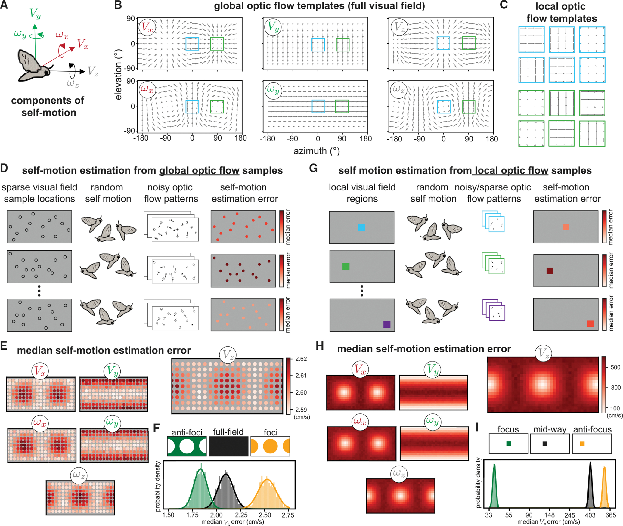
(A) We consider the optic flow generated by 6 components/directions of self-motion including translation and rotation, illustrated for a moth.
(B) Idealized optic flow templates for recovering each component of self-motion in a spherical environment are shown across the full visual field.
(C) For the blue and green regions highlighted in (B), we show the local flow templates for a 10° square region under a tangent projection. A small field of view can lead to a high degree of similarity between translation and rotation template patches (e.g., VX and ωY look very similar locally at these two positions but are more distinguishable with the full field of view). Arrowheads for the templates located at foci of expansion/contraction have been scaled up for visibility.
(D) To model self-motion estimation from sparse, noisy optic flow across the full visual field, we randomly sampled 60 visual field locations (of 180 predetermined possible locations) and calculated the median absolute self-motion estimation error for each component. Once a sample set was chosen, self-motion components were drawn uniformly at random from −1 to 1 (m/s for translation and rad/s for rotation), and additive Gaussian noise of standard deviation of 0.25 (relative to a maximal per-component flow magnitude of 1) was applied to the resulting flow vectors. The environment was modeled as a 1-m radius sphere. Each row illustrates one iteration of the model: we ran 10,000 iterations with different sample locations each time, and each iteration included 10,000 random self-motions for computing the median absolute error. Color bars indicate the median self-motion estimation error associated with each sample set. We then computed the overall median absolute error (median of medians) associated with each visual field sample location across all iterations.
(E) Heatmaps show the overall median absolute errors associated with each sample location for each self-motion component, with VZ plotted larger for visibility. The heatmap ranges for the other components are: VX (2.59,2.61), VY (2.94,2.99), ωX (1.48,1.50), ωY (1.68,1.71), and ωZ (1.48,1.50).
(F) Histograms illustrate the median VZ estimation error when 50% of the sample locations were used. These 50% could be spread evenly across the visual field (black), concentrated away from the VZ foci of expansion/contraction (green) or concentrated at these foci (orange). The anti-focus spatial bias leads to better estimates. We fitted each distribution with a Gaussian and computed the effect size (the difference between the means normalized by the pooled standard deviations) between the full field and biased samples as follows: anti-foci versus full field = −3.6; foci versus full field = 5.0.
(G) To model self-motion estimation from sparse, noisy optic flow using contiguous local visual field regions similar to receptive fields, we repeated this analysis on small, spatially contiguous regions. Each contiguous region subtended a 10° square and contained up to 100 contiguous optic flow samples, each of which had a 67% chance of being deleted after noise was added, with self-motion and additive noise sampled as before.
(H) Heat maps of the resulting median absolute errors. The heatmap ranges for the non-VZ translation components are the same as the VZ plot, and for the rotation components, they range from 20 to 350 deg/s.
(I) Histograms illustrate the median VZ estimation error (log-spaced) for the best local region (located at the VZ focus), the worst local region (located at the antifocus), and a region mid-way between those two. Effect sizes are as follows: focus versus mid-way = −64.8; anti-focus versus mid-way = 9.2.
Self-motion can be recovered perfectly if these templates match the environmental geometry, optic flow signals are available throughout the visual field, and nothing else in the environment is moving. Real optic flow fields, however, are rarely dense or clean. Sparsity in natural optic flow fields follows from the sparsity of spatial and temporal contrast.47–49 External noise is caused by motion cues in the environment, such as particles moving through air or water, swaying vegetation, moving animals, and optical effects like caustics and shadows. To examine the effects of noise and sparsity on spatial biases, we selected self-motion velocity components uniformly at random, synthesized optic flow samples, added Gaussian noise, and sparsified (by setting both sample and template values to zero at random locations). We initially assume the animal can move with six degrees of freedom (DOF) in a spherical environment with spatially uniform noise, then consider variations on each of these conditions (see figure captions for simulation details). We show that some regions are more useful than others in each of these conditions. This observation holds whether the full visual field is used or only a small contiguous local region is visible.
To evaluate self-motion estimation from the full visual field (global optic flow), we iteratively sampled optic flow across random sets of locations in the visual field and combined the self-motion estimation error across all sample sets (Figure 1D). This approach allows us to examine how each location in the visual field contributes to self-motion estimation, regardless of which other locations it is combined with. The median absolute error in all components of self-motion show small but consistent spatial variations (Figure 1E). Regions with smaller signal-to-noise ratios based on flow magnitude in the global templates (foci of expansion and contraction) are associated with larger errors, and regions with higher signal-to-noise ratios are associated with lower errors, consistent with the results derived from an internal noise model analyzed in Franz and Krapp.37 Importantly, sampling the set of low error locations results in better self-motion estimation than the same number of samples distributed evenly across the visual field. This is demonstrated in Figure 1F for forward translation (VZ). Selecting only the high error samples results in worse forward translation estimation (Figure 1F). We make no claims of optimality for this sampling strategy, instead noting that even naive use of error patterns can generate useful spatial biases.
Next, we restrict sampling to small contiguous regions of the visual field similar to individual receptive fields (RFs) (Figure 1G). In each region, we consider the self-motion estimation errors resulting from these isolated, contiguous samples (local optic flow). Note that the templates for these local regions are less distinct for each component than the global templates are (Figures 1B and 1C), such that the local self-motion estimation problem is generally less well conditioned. This leads directly to a reversal in the pattern of high and low error locations compared with the global sampling strategy, as local condition number has a greater impact than signal to noise (Figures 1H versus 1E). The errors are overall much higher for the local samples and the advantage of spatial biasing is amplified in this case (Figure 1I). Thus, while the visual ecology of different animals can vary widely, if natural flow cues tend to be sparse and noisy, then there will be an advantage for individuals that prioritize informative regions of the visual field.
Using this simulation and estimation framework, we will next evaluate the impact of behavioral and environmental factors on the relative accuracy of self-motion estimates derived from sampling locations across the visual field. We focus on the estimation of forward translation velocity (VZ) and heading direction (tan−1(VZ/VX)), because these are particularly ecologically relevant aspects of self-motion.
Behavior: Self-stabilization improves performance and shifts local spatial biases
Organisms are not entirely in control of their motion, particularly flying or swimming animals that navigate through moving air or water currents. However, many animals stabilize in several dimensions of motion, which simplifies the problems of self-motion estimation and control. This is particularly true for visual systems that rely on localized regions that suffer from template ambiguity. Motion-limiting behaviors can eliminate these ambiguities.
Here, we consider two behavioral simplifications. First, an animal might remove all self-motion other than forward translation (VZ; Figure 2A). In this case, there is a reduction in overall error, and there is still a clear advantage for spatially biased sampling. In this highly simplified setting, many local regions provide near-optimal performance (black and green overlap, bottom). The higher error regions occur primarily at the foci of expansion/contraction. With no ambiguity between templates in the local regime, the problem is perfectly conditioned, and signal to noise alone drives estimation errors, matching the global regime. The resulting spatial pattern of errors is a complete reversal of the local estimation error pattern for an animal moving with 6 DOFs (Figure 1H). While moving in only one direction is infeasible in most natural settings, this example illustrates that the motion behaviors of an animal are highly relevant in shaping their optimal spatial biases, particularly when optic flow is sampled locally.
Figure 2. Animal behavior and environment shape spatial biases.
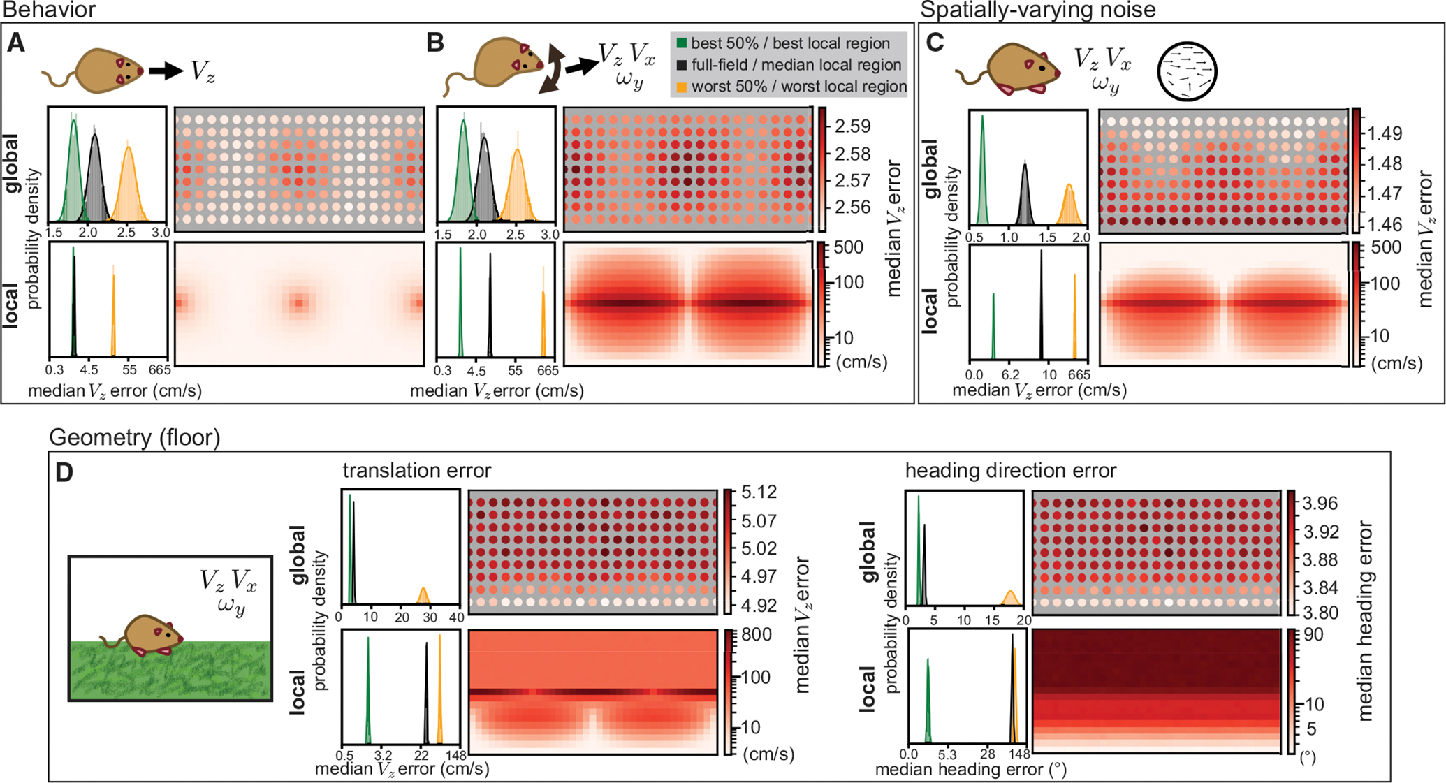
(A) An animal only moving forward removes the ambiguity in local flow templates so that both global and local errors indicate an away-from-foci advantage. Histograms on the left indicate the distribution of median absolute self-motion estimation errors for the best 50%, worst 50%, and full field global samples at matched resolution, and the best, worst, and median local regions over 1,000 simulations of 1,000 self-motion trajectories. Heatmaps indicating median errors are plotted in the same format as Figure 1. All model parameters are the same as Figure 1, except self-motion components other than VZ were all set to zero and a 1 DOF estimation applied. For the local optic flow, both the best and median regions are associated with very low error, resulting in a high degree of histogram overlap.
(B) An animal translating and rotating in a plane sees higher errors and expanded regions of ambiguity. All model parameters are the same as Figure 1, except self-motion components other than VZ, VX, and ωY were all set to zero and a 3 DOF estimation applied.
(C) When noise varies linearly from none at 90° elevation to a maximum at −90° elevation, low error regions are shifted upward. All model parameters are otherwise the same as (B), and maximum noise had a standard deviation of 0.25 (relative to a maximal per-component flow magnitude of 1).
(D) When the environment is a floor plane rather than a sphere, VZ error explodes at and above the equator. Heading estimates remove the depth ambiguity in translation component magnitude by comparing VX and VZ estimates, eliminating azimuth dependence for a pure lower field bias. All model parameters are the same as (B) except for the scene geometry, which is modeled as a flat floor 1m below and an infinitely far away wall in the upper visual field. Note that histograms and heatmaps for local errors in this figure are all on a log scale to account for the larger variability associated with different environmental settings.
For a terrestrial animal, or a swimming or flying animal that stabilizes its motion to a plane, three degrees of freedom may be a more reasonable simplification: forward translation (VZ), lateral translation (VX), and yaw (left/right) rotation (ωY) only. These can occur simultaneously, as when forward body motion is combined with a rotation of the head. This behavior, illustrated in Figure 2B, does not affect the spatial error patterns for global optic flow, but for local sampling, it leads to high estimation error in regions to the left and right sides, particularly along the equator where yaw rotation can be confused for forward or lateral translation. Elsewhere in the visual field, self-motion can be recovered reliably from local optic flow.
Environment: Spatially varying noise and scene geometry drive spatial bias
The previous examples showed environments with spatially uniform sparsity and noise. In reality, natural environments likely feature statistical regularities in the availability and reliability of optic flow signals across space. Figure 2C shows the result for estimating 3DOF motion in a sphere where the noise increases linearly from top to bottom. This shifts the low-error regions upward while maintaining the general spatial pattern for both globally and locally derived estimates. Spatial variations in sparsity have similar effects (not shown). When noise and sparsity are not present, all regions of the visual field are equally, perfectly informative; hence, the spatial distributions of noise and sparsity in an environment are fundamental drivers of error patterns in self-motion estimation.
The previous examples also all modeled the environment as a sphere. This could be considered a reasonable simplification for the ecological niches of some animals, like insects that fly through dense foliage. However, many natural environments are better modeled as having a ground plane that creates systematic depth variation as a function of elevation in the visual field.37,50,51 Figure 2D shows the different error patterns that emerge as a result of ground plane geometry for 3DOF motion. Here, we assume that all points above the ground are too distant to provide motion parallax cues so that forward velocity estimation errors shift from an elevation-symmetric pattern in the sphere (Figure 2B) to strongly favoring the lower field (Figure 2D). The worst errors in local VZ estimates occur at the equator toward the front/rear of the animal, where the small expected optic flow magnitude can lead to very large and incorrect predictions if rotation cues are mistaken for translation. Nonetheless, broad regions of the lower field are useful for determining the speed of forward translation.
When scene geometry is only known up to a scale factor, translation magnitudes cannot be accurately recovered, as a scene point moving fast and far away will generate the same optic flow as one moving slower and closer. This issue can be mitigated by comparing translation components (for example, by taking the heading angle) for a depth-independent estimation of self-motion. In the floor geometry, errors in horizontal heading angle estimation are also lowest in the lower visual field (Figure 2D, right). Spatial biases in heading error also have less azimuth dependence, as the foci for VX and VZ, both of which are needed to recover horizontal heading, are offset by 90°.
Simulations predict advantage to spatial biases of self-motion estimation
In summary, animal behavior, environmental noise, scene geometry, and sampling strategy all influence spatial patterns of error for an animal attempting to infer its self-motion from optic flow measurements. These error patterns can be used to easily generate a spatially biased sampling pattern that outperforms uniform sampling. The most informative regions of the visual field will differ for organisms in different niches, but with sufficient context, we should be able to quantify the advantage of a spatial bias for a particular animal. Next, we will apply this framework to the larval zebrafish and compare the predictions based on a model of these factors with direct measurements of spatial biases in the OMR.
Larval zebrafish optomotor swimming is driven by the lateral lower visual field
Larval zebrafish OMR is driven preferentially by moving stimuli in the lateral lower visual field,34 and pretectal neurons tuned for self-motion direction tend to have receptive fields in the lower visual field.24 To explore this behavior in more detail, we employed a spherical arena of over 10,000 individually controlled LEDs38 and displayed a series of moving stripe patterns to head-fixed larval zebrafish (Figures 3A, 3B, and S1A). The new arena allowed greater flexibility of stimulus patterns, larger coverage of the visual field, and higher spatial resolution for mapping of the spatial biases in the optomotor drive.
Figure 3. Larval zebrafish optomotor swimming is driven by the lateral lower visual field.
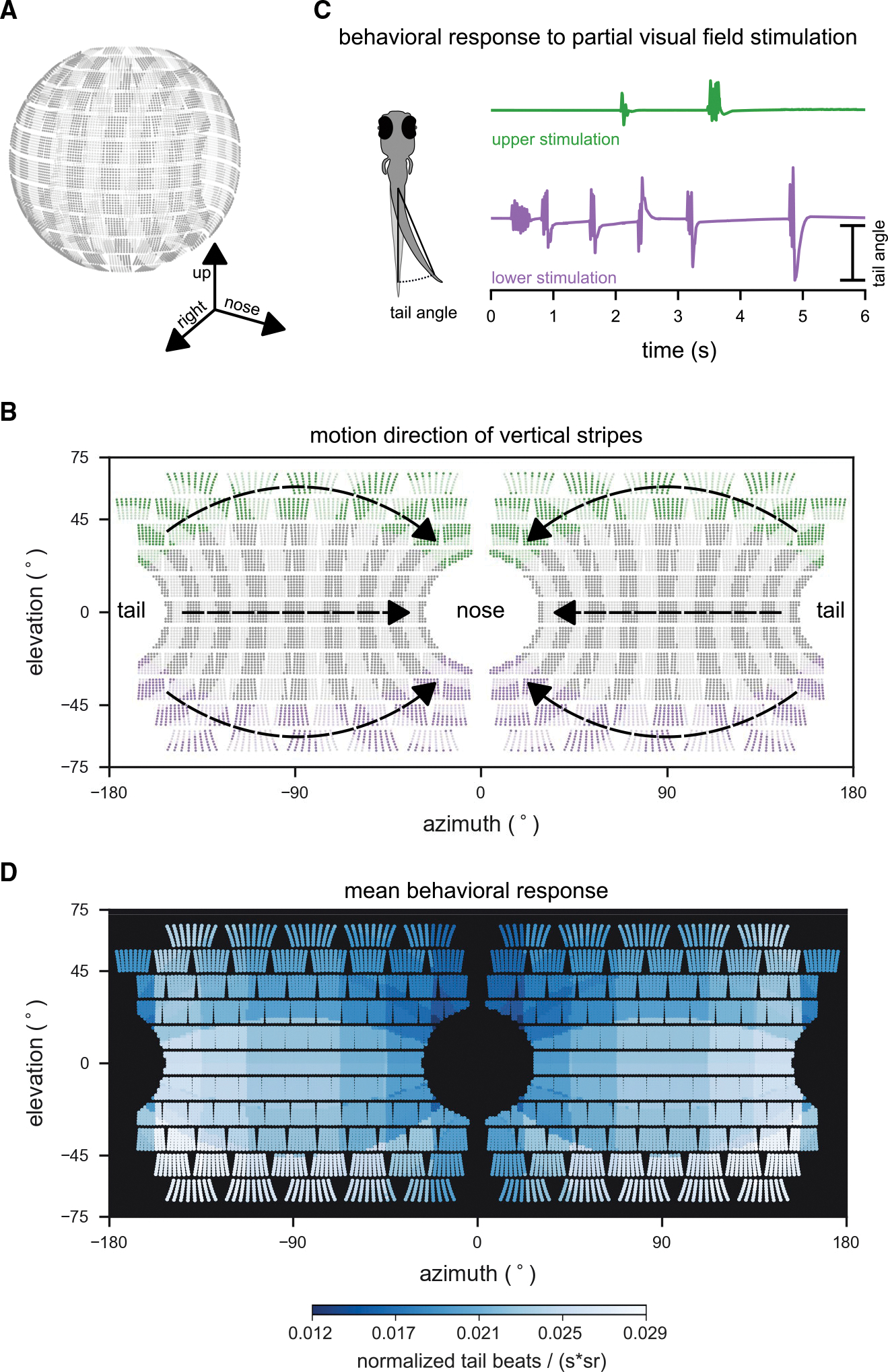
(A) Layout of individual LEDs in our spherical visual stimulation arena. The visual stimulus consisted of a pattern of vertical bars meant to simulate the fish swimming through a pipe with transverse stripes. Fish were placed in the center of the spherical arena, thus allowing for stimulation of an extended range of elevations (almost 140° × 360° of its visual field).
(B) During individual trials, stripes in different regions of the visual field were moving (example areas marked green or purple), whereas the rest remained static. Stimulus motion was from back to front, providing the percept of backward drift to the fish.
(C) Tail bend angles were measured for each recorded video frame to calculate behavioral responses to different stimulus locations. Fish generally responded more strongly to motion in the lower (purple trial), than in the upper (green trial) visual field.
(D) Heatmap color indicates the strength of the OMR to motion stimuli in different parts of the visual field. OMR drive was strongest for motion in the lateral lower visual field. To quantify the behavioral response, the number of tail beats per unit time was averaged over repeated trials for each fish, normalized by the fish’s maximum response to any of the stimuli, and scaled by the inverse of the area (in steradians) that was active (i.e., moving) for each stimulus to account for effects of stimulation area size on response strength. Responses were then combined into a single average across fish (n = 8 fish). Motion stimuli covered 19 different combinations of positions and steradian sizes in visual space.
See also Figure S1.
We consider tail beat responses to patterns that simulated backward drift in a tunnel (Figures 3B and 3C). These patterns were presented over 19 visual regions (Figure S1B), and the responses were combined to map the regions of the visual field that most effectively elicited an OMR (i.e., tail beats) (Figure 3D). These new data confirm and extend the conclusion that the fish preferentially use the lateral lower visual field to estimate self-motion signals pertinent to the forward swimming OMR (although substantial variation was observed from fish to fish; Figures S1C and S1D).
We now test the hypothesis that this spatial bias in OMR behavior reflects an adaptation to optic flow signals in the fish’s habitat. Combining knowledge of the fish’s behavior and visual system, ecological assessments of the zebrafish’s habitats, and a novel optic flow dataset, we model the factors relevant to zebrafish self-motion estimation. First, we use a natural video dataset to create a generative model of local flow regions observed in the zebrafish habitats, enabling an exploration of spatial biases in simulation. Then, we confirm simulation results by using the dataset videos directly to characterize elevation-dependent performance in self-motion recovery from natural optic flow recordings.
Dataset from the zebrafish habitat
We collected a video dataset from natural zebrafish habitats (Figures 4A and 4B; Table S1), which can be found in shallow freshwater environments throughout South Asia.52 Videos were collected using a waterproofed 360° camera mounted to a robotic arm for controlled motion trajectories: translations forward/backward, translations sideways, translations at 45°, clockwise/counterclockwise rotations, and circular turns (Table S2). A sample video frame from each site is shown in Figure 4C, with short video samples in Video S1. All frames and code used in the analyses are publicly available.53,54
Figure 4. A model for natural optic flow statistics during zebrafish self-motion.
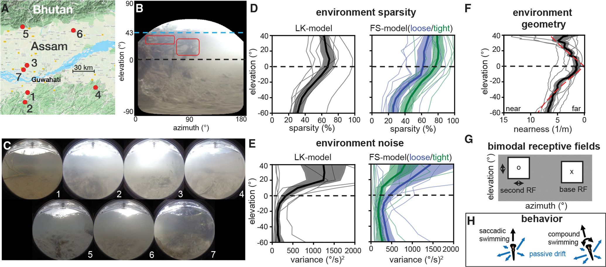
(A) Seven sites in the native range of the zebrafish were sampled, see Table S1 for details. Image from Google Maps.55
(B) An equirectangular projection of a sample frame shows elevation-dependent sources of signal and noise.
(C) Frames from each site summarize visual variation across the native range.
(D) Optic flow sparsity at individual sites (thin lines) and averaged across the dataset (thick lines, ±SEM in filled region) show high sparsity near and above the equator. This pattern holds across motion measurement algorithms (black, blue, and green).
(E) Errors in optic flow, attributed to natural motion within the environment, show higher variance in the upper visual field.
(F) The geometry estimated from optic flow vector magnitudes roughly matches a floor+ceiling model (dashed red) below the water line (~40°). Individual sites, SEM, and mean are plotted in the same manner as in (D) and (E).
(G) Receptive field structure is modeled in spatially separate bimodal pairs. Base RFs were placed in a predetermined grid of locations and paired with a range of possible second RFs.
(H) Two swimming behaviors are considered: saccadic swimming, where forward motion is added to lateral drifting (VZ ~ U[0,1] m/s + (VX,VZ) ~ U[−.5, −.5] m/s) and compound swimming, which additionally includes rotation (ωY ~ U[−1,1] rad/s). For more details, see Figures S1–S3 and S7, Video S1, and Tables S1–S4.
Calibrated camera parameters were used to reproject frames onto smaller planar tangent surfaces, creating image samples analogous to the local flow regions described in the previous section (Table S3). Optic flow was measured using two different algorithms: the Lukas-Kanade (LK) method56 and the Farid and Simoncelli (FS) differentiation method.57 Both methods apply the brightness constancy constraint to spatiotemporal derivatives, similar to the canonical computations thought to underlie motion processing across the animal kingdom.24,58–60 Whereas the LK method performs sparse tracking of informative flow features (e.g., corners), the FS derivative filters were applied to a pre-specified grid of points so that optic flow was computed regardless of the features present. Optic flow measurements were considered valid when features were successfully matched by the LK method and when the condition number and gradient magnitude met appropriate thresholds for the FS method. Since there is no a priori way to select a biologically meaningful threshold on gradients for the larval zebrafish, we consider two luminance gradient thresholds for the FS method, one relatively high (tight) and one relatively low (loose).
Motion sparsity and noise vary over elevation in the zebrafish habitat
The sample in Figure 4B illustrates several elevation-dependent sources of signal and noise typical of shallow aquatic environments. Due to refraction at the water’s surface, light from above the waterline fills the region from +90° to approximately +43° in elevation, known as Snell’s window. This fixed waterline (dashed blue line) often provides very strong optic flow cues, due to the high contrast edge between water and sky and the frequent presence of high scene velocities, but much of this optic flow is caused by the motion of the water surface and is misleading as a self-motion cue. In the portion of the upper field between Snell’s window and the equator (dashed black line), scene texture is somewhat sparse but can be augmented by reflection off of the underside of the water surface (red boxes). In a perfectly still and clear scene, the water surface would mirror the texture of the floor up to Snell’s window. In reality, scattering through turbid water and motion of the surface disrupt this reflection, so that high contrast edges are rare in the upper field. The equator generally lies in a region with very sparse contrast due to long viewing distances through turbid water. The lower field tends to provide much more visual contrast due to the texture and nearness of the floor. Optic flow in this region is not always informative to self-motion, though. For example, the bright lines visible are caustics caused by local focusing of sunlight by the water surface, and they provide a consistent but misleading optic flow field caused by water motion.
The video dataset was first used to determine an appropriate noise and sparsity model for the native habitat of the zebrafish. We focus on quantifying two features of optic flow: signal sparsity, modeled from the portion of valid flow measurements, and environmental noise, modeled from the deviation from ground truth flow fields in rotation videos. Elevation-dependent measurements were made covering a total visual area from −80° to +60°.
We found that signal sparsity was lowest in the lower visual field, increased up to the equator, and then dipped slightly with increasing elevation (Figure 4D). This trend held across optic flow calculation methods. The FS threshold can be set to match LK sparsity with more noise (loose, blue) or recover accuracy at the cost of higher sparsity (tight, green). We also found that the noise variance was larger in the upper visual field (Figure 4E). To accurately capture the high kurtosis of the flow errors, we fit the error distributions with a generalized zero-mean Gaussian at each elevation (Figure S2; Table S4). These models were used to generate optic flow simulating the sparsity and noise of the zebrafish habitat at each elevation. We report the results from the LK optic flow method in the main manuscript and include the results from the FS methods in the Supplement. The findings do not differ meaningfully between the different methods.
Shallow aquatic scene geometry in the zebrafish habitat
We adopt a simplified and widely applicable geometric model for a shallow underwater environment: a floor below the fish and a ceiling above, with features above the waterline too distant to provide accurate translation cues. We compare this model with estimates derived from translational trajectories in Figure 4F, based on elevation-dependent nearness (1/distance).
Larval zebrafish receptive fields for optic flow
We sampled optic flow in local regions spanning 40° × 40°, similar to larval pretectal and tectal RF sizes.34,61 RFs were placed without reference to the larval zebrafish field of view (approximately 160° per eye22) or binocular overlap. Each model RF contained a set of up to 25 flow measurements, modeling inputs from retinal ganglion cells with smaller receptive fields.62,63 RFs were considered in bimodal pairs (Figure 4G), as these bimodal pairings (i.e., two spatial regions per RF) are common in the larval zebrafish.24 In the larval zebrafish, these bimodal pairs tend to prefer a specific translation direction, with each mode offset symmetrically from the preferred translation axis and positioned away from the foci of that translation. By considering a grid of base RF locations and examining how performance varies when these are paired with a second RF across all potential locations in the visual field, our analysis predicts such symmetric equal-elevation pairs without a priori assumptions beyond the size, density, and bimodality of RFs.
Larval zebrafish swimming
Larval zebrafish display a diverse repertoire of visually driven swimming behaviors,64,65 but most of their self-generated translation is restricted to the horizontal plane.66,67 Using the vestibular system, the fish balance against roll and pitch;68,69 hence, we ignore these degrees of freedom as well. For underwater and flying animals, there is growing evidence for “saccadic locomotion” strategies, in which rotational movements (i.e., turns) are performed quickly and in temporal separation from translational movements, likely simplifying self-motion estimation.70–73 Thus, two swimming behaviors are considered here: saccadic swimming in which forward swimming is combined with slower passive horizontal drift due to water currents (Figure 4H, left) and compound swimming that additionally includes horizontal rotation (Figure 4H, right).
Simulation results show advantage for lateral lower visual field bias
Following the models described above for the environment sparsity and noise, scene geometry, RF structure, and swimming behavior, we simulated realistic local optic flow measurements across the visual field and assessed their informativeness for self-motion estimation using the framework described previously.
We found that the lowest forward translation (VZ) estimation errors were associated with RF pairs in the lateral lower visual field for saccadic swimming behavior. The lowest error occurred when the base and second RF were located at an elevation of −60° and has azimuths of 90° and −90°, respectively (marked with an x and o in Figure 5A, left). The heatmap shows the median absolute VZ error for all second RF locations paired with the best base RF location: there is a general trend of lower error in the lower visual field. This trend is not unique to the base RF shown. For each base RF, the error as a function of second RF elevation trended downward toward the bottom of the visual field (means shown in middle panel of Figure 5A, full results in Figure S4). Indeed, error was minimized by moving both the base and second RFs into the lower visual field (i.e., the green line has the lowest errors and slopes right-wards). The error in heading direction as a function of RF elevation matches these elevation-dependent effects. Examining the mean VZ error over azimuth (Figure 5A, right) across all second RF elevations demonstrates the importance of lateral RF placement. Here, we show just the errors for the best base RF elevation (−60°). Overall, errors tended to be minimized for RFs placed at azimuths of +90° and −90°.
Figure 5. The visual ecology of the larval zebrafish generates lower translation estimation errors in the lateral lower field.
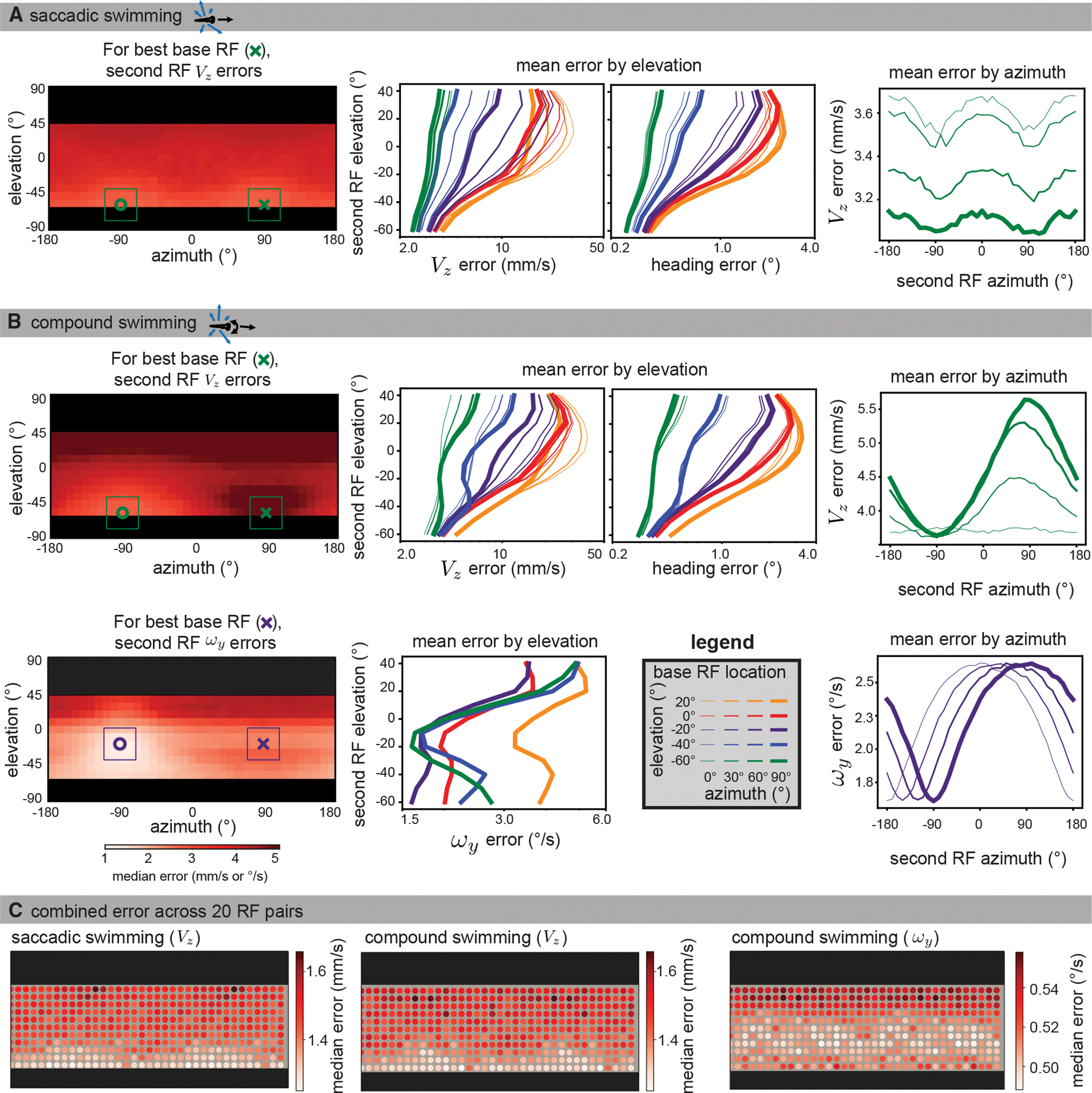
Data were simulated using naturalistic models of signal sparsity and noise, environment geometry, RF size and structure, and swimming behaviors. For each possible base RF location (see legend in B), median absolute errors were computed for 10,000 iterations across all second RF locations.
(A) Left: for saccadic swimming, the lowest error occurred when the base and second RF were located at an elevation of −60° and had azimuths of 90° and −90°, respectively. The plot shows a heatmap of the median absolute VZ error over across all second RF locations for the best base RF, and the single best base/second pair is indicated with an x and o. middle: for VZ and heading error, median absolute errors are averaged across azimuths to isolate elevation trends for each base RF location (colors indicate base RF elevation, line thicknesses indicate base RF azimuth). Both metrics show that translation is best recovered by RF pairs in the lower visual field. Right: When averaging across elevation for azimuth trends, the lower field base RFs tend to be best matched with a second RF at ±90° azimuth. For clarity, we only plot the results for the best base elevation (−60°).
(B) For compound swimming behavior, local translation errors (top left) show more extreme penalties for same-side sampling due to ambiguity with rotation. Elevation trends (top middle) are largely unaffected, other than an increase in average error, but azimuth trends (top right) show a strong advantage to sampling the lateral region on the other side of the body. The azimuth and elevation of the best individual pair are the same as for saccadic swimming. For rotation estimation (bottom), the lower field advantage is less strong, and the best performing bimodal RF (bottom left) appears at −20° elevation. Elevation trends (bottom middle) show strong performance throughout the lower field, whereas azimuth trends show no clear advantage to lateral regions, instead suggesting an azimuth separation of 180° minimizes error (bottom right). Full error maps can be seen in Figures S4 and S5, with a comparison across flow calculation methods shown in Figure S6.
(C) To characterize the performance across the visual field, we followed a similar method to the global method described in the previous section. Instead of a location sample corresponding to a single flow vector, we sampled sets of 20 RF pairs, with one centered at the sample location and the other 180° away in azimuth at the same elevation. The median absolute error over 1,000 estimates is shown for each of the motion directions from (A) and (B). Again, we see better performance in the extreme lower field for translation estimation (left, middle) and in the mid-lower field for rotation (right).
See also Figures S4–S6.
The results for translation estimation were similar for compound swimming (Figure 5B, top row). For RF azimuth, there was an extra boost (lower error) associated with placing the second RF on the opposite side of the nose, since this location is helpful for disambiguating optic flow caused by translation versus rotation. Rotation estimation errors were minimized with samples placed closer to the equator within the lower field (Figure5B, bottom row) and separated by 180° in azimuth. For rotation, the elevation of the best pair was −20° (purple lines), although the error averaged across all azimuths was slightly lower for the lowest base RF (−60°). The equatorial bias for rotation reflects the tension between the higher quality optic flow signals in the lower field and the geometric advantage of the distant equator for rotation estimation (the large distance removes ambiguities with translation signals). Full error maps are in Figure S5. The results shown in Figure 5 all use the LK-based noise model; similar results are shown for the two FS-based noise models in Figure S6.
We then considered the performance of combined bimodal RFs using an analysis similar to the global optic flow sampling shown in Figures 1 and 2. Rather than randomly sampling individual flows, we randomly sampled sets of 20 bimodal RFs, enough to cover the entire visible region when evenly spaced. The heatmaps in Figure 5C show the resulting median absolute errors associated with each spatial location in the visual field. The lower errors in the lateral lower field for translation, and toward the equator for rotation, are preserved even when multiple RFs are incorporated.
Comparing translation error across the two behavior types, we see that the lowest errors are comparable, but the highest errors are worse for the fish that combines translation with rotation while swimming. In noisy natural habitats, we infer that motion-limiting behaviors like saccadic swimming may reduce the advantage of spatial biases and allow more accurate self-motion estimation from less complex visual systems or more challenging scenes.
Results with real optic flow reiterate lower visual field bias
The previous section asserted a generative model of optic flow based on separate models of the scene geometry, signal availability, and noise in the native habitat of the zebrafish. This allowed for flexibility in our analysis: we could consider arbitrary velocities and simulate different locations across the visual field without loss of resolution or distortions in the camera. However, real optic flow samples from the video dataset provide a better reflection of higher order statistics of signal and noise, such as the spatial correlation of strong contrast cues or the presence of coherently moving distractors and scene geometry, which determines the tradeoff between translation and rotation cues. Thus, we turn to an analysis of real optic flow samples. Bimodal optic flow samples were collected from the high-resolution lateral regions of omnidirectional videos during several translation and rotation trajectories (see Table S2). Each flow sample contained two 40° × 40° regions, centered at ±90° in azimuth and matching in elevation. Each bimodal sample was used to estimate self-motion, both in isolation and combined with samples from other elevations in the same video frames.
Figure 6 shows the elevation-dependent errors for forward translation (Figure 6A), heading direction (Figure 6B), and rotation speed (Figure 6C) from these data. The first column compares the estimation errors from single-sample estimates (gray line, illustrated with inset of visual field) with the error from using all elevation pairs in each frame (dashed black line). In general, single-elevation estimates perform less well than using all of the data, but in each case, there are elevations where a single sample is as effective or more effective than using the entire field. These correspond to the high-performing elevations in our simulation: −60° for translation and −20° for rotation. The rest of the visual field contains many misleading flow vectors, ultimately doing more harm than good. We also considered the effect of excluding single-elevation samples from the full field (Figure 6, second column). For both translation and rotation, ignoring data from the lower field reduces performance but ignoring data from the upper field improves it.
Figure 6. Ignoring the upper field improves motion estimates from optic flow measured in the native habitat of the zebrafish.
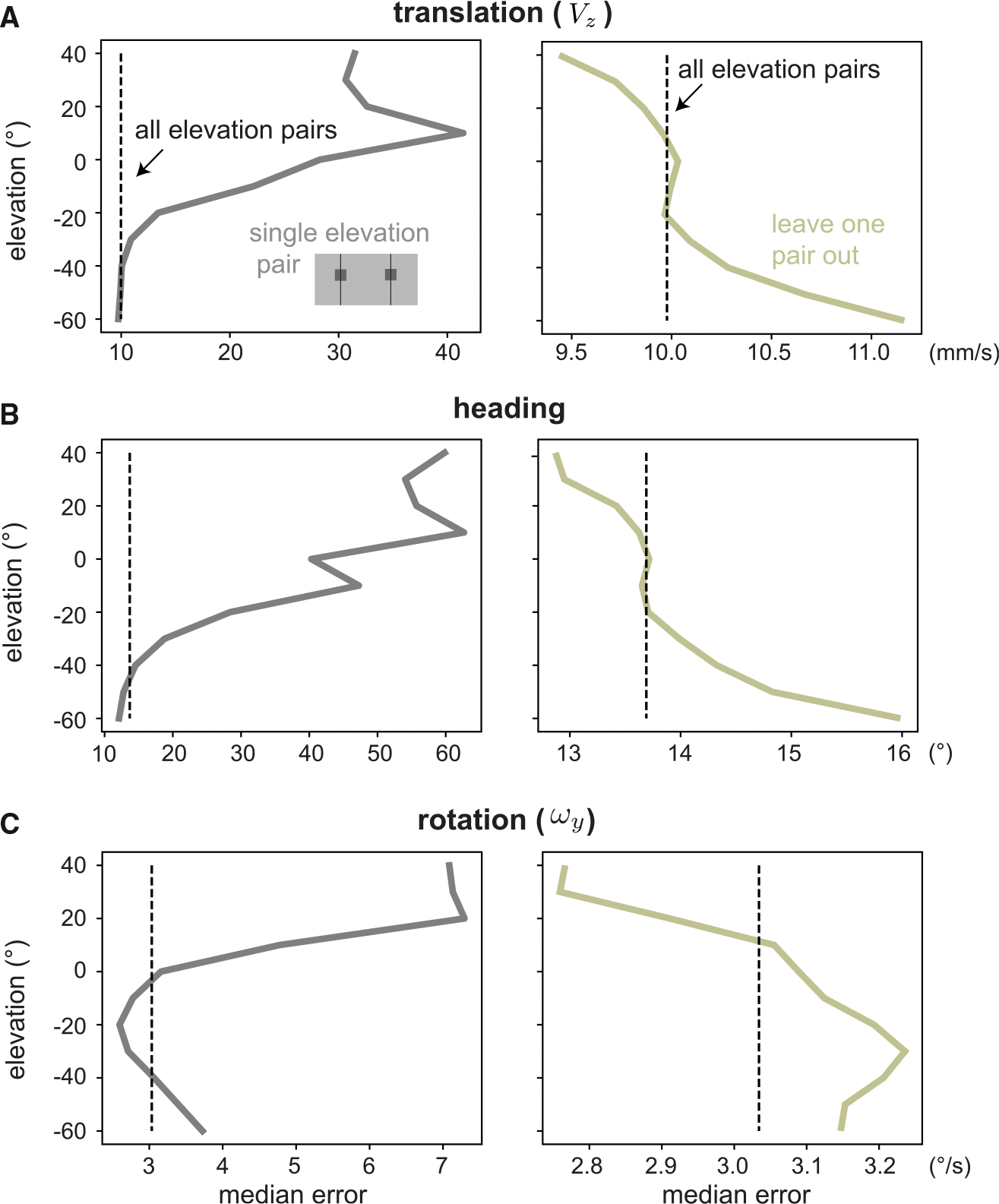
We demonstrate the value of spatial biases by showing an advantage to excluding elevations from self-motion estimation across our dataset of natural optic flows. For velocity distribution and dataset size, see Table S2.
(A–C) We consider forward translation (A), heading (B), and rotation (C) errors for single RFs pairs, comparing with a baseline of using all elevations (dotted vertical line). When using a single elevation (first column), the best regions predicted by our simulations are equal to or outperform the baseline. When all but one elevations are used (second column), removing lower field samples damages performance while removing upper field samples improves it.
DISCUSSION
Taken together, these results suggest that spatial biases in optic flow sampling represent an adaptation to reliably estimate self-motion in noisy natural environments. Here, we highlight how the current approach can be extended and contextualize our findings in the broader literature on motion processing in the zebrafish.
Spatial resolution across the visual field
The retinas and brains of many organisms feature anatomical and functional spatial biases that are not yet fully understood. These additional spatial biases can be readily incorporated into the current framework to explore new questions. For example, our predictions for a lower field bias in rotation estimation in larval zebrafish appears to contradict a recent study showing more robust behavioral responses to rotational optic flow in the upper visual field.38 It was hypothesized that higher cone density in the upper visual field may contribute to this rotational spatial bias. We can test the hypothesis that variation in retinal resolution is sufficient to overcome elevation-dependent noise patterns in rotation estimation. To do so, we modeled the retinal resolution bias by reducing sparsity by a factor of 4 for elevations above the equator, on the assumption that more sample locations increases the probability of detecting sparse scene points. We then considered a base RF in the upper visual field, placed laterally and at a 20° elevation to stay fully below the waterline, and examined the mean self-motion estimation error across azimuths for each possible elevation of a second RF (Figure 7). For rotation, the best second elevation moved into the upper visual field, whereas for translation, the best second RF elevation remained in the lower visual field, consistent with the spatial biases seen in both behavioral responses. This preliminary observation suggests that anatomical biases can be powerful enough to change the reliability of optic flow across space. Although the upper visual field may not be a more reliable source of self-rotation information per se, other behavioral pressures (e.g., hunting, predator avoidance) may drive photoreceptor density in this region and affect downstream optic flow processing for self-motion.74 These interactions across different spatial biases and different anatomical/functional stages would be a fruitful direction for future work. Based on this analysis, we might predict, for example, that genetically diverse but closely related species, such as cichlids, should also have different spatial biases in optic flow processing. These biases could be predicted independent of behavioral experiments by taking similar measurements from their anatomy and environment.75
Figure 7. Spatially varying resolution of the front end of the sensory system can shift rotation bias.
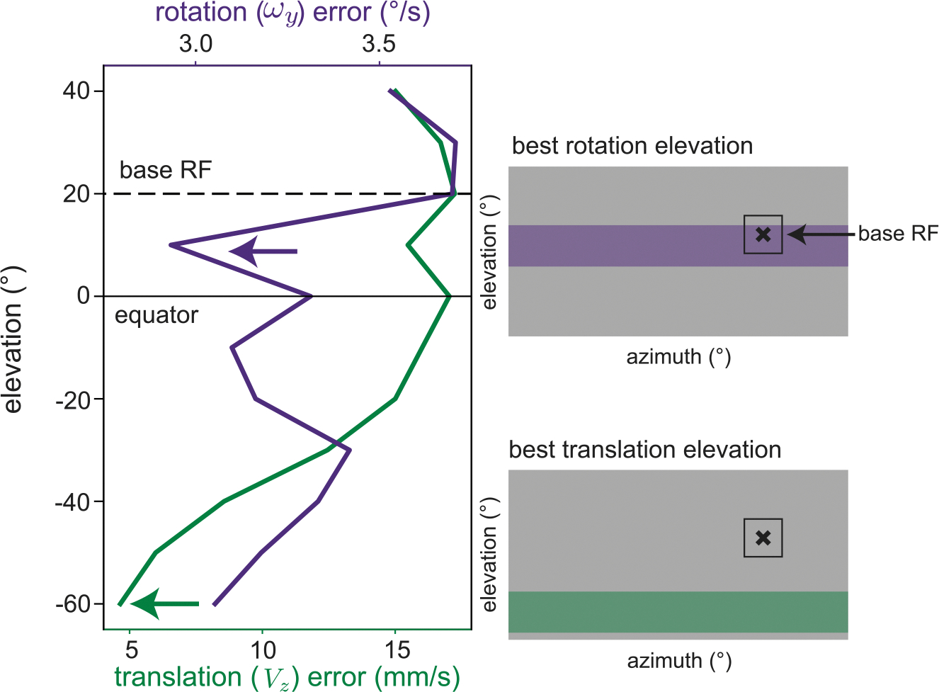
Beginning with the compound swimming setting in Figure 5, we modified our sparsity model to increase sample probability by a factor of 4 in the upper visual field, as a proxy for higher retinal resolution. In this setting, a base receptive field located at 20° elevation (black dashed line) and 90° azimuth is better paired with another upper field RF for rotation (purple arrow) while still benefiting from a lower field partner for translation (green arrow). Compare with Figure 5D in which both types of motion estimation show lower error in the lower field. Spatial variations in anatomical resolution may be responsible for a slight upper field bias observed in rotation responses in the larval zebrafish.
Behavioral adaptation and energy allocation
An important driver of sensory and motor systems throughout the animal kingdom is metabolic efficiency. In addition to the energetic demands of processing sensory information, many animals also sample the world using eye, head, and body movements. Complex energy tradeoffs determine ideal motion patterns for optimal sensing.44 It is perhaps no surprise then that spatial biases in optic flow responses emerge as being particularly important for understanding highly energy-constrained animals such as insects and simple vertebrates such as the larval zebrafish.27,29,30,32,33 In more complex-brained animals, like humans, such spatial biases are seen in low-level dynamic tasks like keeping us upright as we stand31 and walk,14 which may require faster and more efficient visual processing. Limitations on energy and response time may drive organisms to rely on heuristics and clever tricks over higher-level scene processing.
In this context, it is interesting to consider whether the larval zebrafish visual system is adapted to larval or adult swimming behavior. Since the larval brain is more computationally constrained than the adult brain (many additional pretectal neurons will be added during ontogeny), we believe that it is likely that larvae are specifically adapted to larval behavior. Indeed, larval behavior has characteristic properties, such as swimming in discrete bouts, that may facilitate self-motion estimation with simple circuits.64 For example, during quick turns, larvae turn at a speed of about 30,000°/s.76 Since retinal speeds above 100°/s are unlikely to evoke motion responses in retinal ganglion cells,77 such high speeds are likely ignored by the fish when estimating self-motion, in favor of using the slower components of motion following the initial acceleration. Bouting thus likely matters for motion processing strategies, since it structures locomotor trajectories to be (1) mostly saccadic and (2) sometimes too fast for the associated optic flow to be perceivable. However, the spatial biases explored in the current report appear largely robust to different swimming behavior models, suggesting that both larval and adult zebrafish may benefit from the same spatial biases in optic flow processing. We therefore speculate that developmental plasticity of the lateral lower field bias may be relatively low, on the basis that it need not adapt between larval and adult behavior.
Conclusions
The self-motion estimation problem has been solved across the animal kingdom with a widespread reliance on spatially biased optic-flow processing, shaped by the combination of brains, behaviors, and backdrops that determine each species’ unique visual ecology. The larval zebrafish has emerged as a model organism in neuroscience, with a body of work describing their genetics, brain structures, and single-cell responses. The use of such model organisms is a powerful technique for moving neuroscience forward, but it must be done carefully, with a full understanding of the context that has driven their neural and behavioral responses. For example, both humans and zebrafish exhibit a lower field bias in optic flow responses, but our environments, behaviors, and receptive fields are drastically different. Rather than simply concluding that organisms benefit from lower field biases in general, we must consider that they may have arrived at similar solutions for solving diffent self-motion estimation problems.
STAR★METHODS
RESOURCE AVAILABILITY
Lead contact
Further information and requests for resources should be directed to and will be fulfilled by the lead contact, Emma Alexander (ealexander@northwestern.edu).
Materials availability
This study did not generate new unique reagents.
Data and code availability
The video dataset and the zebrafish behavioral data have been deposited at Zenodo and are accessible via the URL in the key resources table.54 All original code is on Github and accessible via the URL in the key resources table.55 Any additional information required to reanalyze the data reported in this paper is available from the lead contact upon request.
KEY RESOURCES TABLE.
| REAGENT or RESOURCE | SOURCE | IDENTIFIER |
|---|---|---|
|
| ||
| Deposited data | ||
|
| ||
| Custom Python code and information about field sites | This paper | https://doi.org/10.5281/zenodo.7120876 |
| Video dataset | This paper | https://doi.org/10.5281/zenodo.6604546 |
|
| ||
| Experimental models: Organisms/strains | ||
|
| ||
| Tg(elavl3:nls-GCaMP6s)mpn400 | Förster et al.78 | ZFIN ID: ZDB-ALT-170731-37 |
| Tg(elavl3:H2B-GCaMP6f)jf7 | Vladimirov et al.79 | ZDB-ALT-150916-4 |
| mitfa | Lister et al.80 | ZFIN ID: ZDB-GENE-990910-11 |
|
| ||
| Software and algorithms | ||
|
| ||
| Python 3.8 | python.org | RRID:SCR_008394 |
| Jupyter | jupyter.org | RRID:SCR_018315 |
| Numpy | numpy.org | RRID:SCR_008633 |
| SciPy | scipy.org | RRID:SCR_008058 |
| Pandas | pandas.pydata.org | RRID:SCR_018214 |
| h5py | h5py.org | https://doi.org/10.5281/zenodo.4584676 |
| Opencv (Matlab and Python versions) | opencv.org | RRID:SCR_015526 |
| FFmpeg | ffmpeg.org | RRID:SCR_016075 |
| Matlab 2022a | Mathworks | RRID:SCR_001622 |
EXPERIMENTAL MODEL AND SUBJECT DETAILS
The behavioral experiments with zebrafish were approved by the government authorities (Regierungspräsidim Tübingen) and carried out in accordance with German federal and Baden-Württemberg state law. Eight animals aged between 5 and 7 days post fertilization were used in this experiment. These animals had different genotypes (e.g., broadly expressing a GCaMP calcium indicator using the transgenic lines Tg(elavl3:nls-GCaMP6s)mpn40078 or Tg(elavl3:H2BGCaMP6f)jf779) that were likely heterozygous. The pigmentation ensured high visibility of the animal body against the background in the experiments (animals were likely heterozygous for mitfa80). The sex of zebrafish is only determined at late larval stage and genetic as well as environmental factors affect sex determination81. Therefore, the larvae used in our experiments did not have an (identifiable) sex yet and experiments were thus agnostic to sex.
METHOD DETAILS
Coordinate system
We adopt an East-North-Up, or ENU, geographic coordinate system to represent angular positions around the animal. In this system, all positions are defined relative to the animal’s head, and expressed as azimuth (horizontal angle, with positive values to the right of the animal), elevation (vertical angle, with positive values above the animal), and radius (or distance to the animal). The point directly in front of the animal (at the rostrum) is located at [0°, 0°] azimuth and elevation. Azimuth angles cover the range [−180°, 180°] and elevation angles [−90°, 90°]. Further details are described in Dehmelt et al.38
Estimating self-motion from optic flow
We denote the locations of physical points in the world relative to the eye as X,Y,Z, and we denote the radial distance of these points as r. At each angular location around the animal, with elevation α and azimuth θ in radians, the optic flow associated with a translation of (VX,VY,VZ) and a rotation of (ωX,ωY,ωZ) takes the form:
| (Equation 1) |
| (Equation 2) |
We refer to these as “ideal flows” because they will only occur when motion cues are dense and accurately sensed.
When examining contiguous local regions of the visual field, we consider instead a simplified pinhole camera model with focal length f and a planar sensor, so that world points are projected to pixel locations x = fX/Z, y = fY/Z (note we assume here an imaging plane in front of the pinhole, without loss of generality). In an ideal setting, optic flow on this plane takes the form:
| (Equation 3) |
| (Equation 4) |
These equations illustrate that the optic flow components in both systems can be modeled as weighted sums of optic flow templates, where the weights are translational and rotational components of self-motion and the templates are determined by a combination of location in the visual field, scene depth, and, in the tangent projection, focal length. If the depth of each point is known, we can render the library of six local optic-flow templates for each spatial region corresponding to the six components of self-motion (Figures 1B and 1C). We assume a unit focal length for these local projections, equivalent in the small angle regime to representing x and y in terms of visual angle rather than pixel location. In either setting, flattening the flow samples into a vector and stacking the flattened templates into a matrix A, we can consider the previous equations as
| (Equation 5) |
where is the 6-component self-motion velocity vector. Under ideal circumstances, the templates in A will be linearly independent, so that the velocity of self-motion can be recovered exactly by inverting the system. However, this recovery can degenerate in practice for a number of reasons, for example, when the measured optic flow is too sparse or impacted by other sources of motion. To model noise in optic flow available from natural environments, we initially assume additive Gaussian noise. For the noise model derived for the zebrafish habitat, we use a fitted generalized Gaussian additive noise model (see below).
To model sparsity in optic flow signals, we delete some percent of a signal’s samples at random. The samples must be removed from the calculation, rather than set to zero, because setting only the samples to zero indicates a signal of zero motion. While the sparsity of successfully computed optic flow samples provides a powerful metric for the quality of motion signals available in the environment, it is not clear how the early visual system of the zebrafish would detect and discard the samples we exclude. That is, we do not propose a specific model for how high contrast stationary signals are represented differently from low contrast, subthreshold signals with some motion. We simply assume that a sample with no motion signal is discarded.
This template-based approach for determining self-motion relies on some knowledge of scene geometry because the pattern of the translational templates depends on the distance of points from the animal. It is currently unknown how biological visual systems handle this ambiguity. We employ a plausible model of average scene geometry so that in our simulations the templates precisely match the simulated environment, but when using optic flow data from our video dataset directly the templates are only an approximate match.
General simulations: Global flow samples
To calculate the self-motion estimation errors shown in Figure 1 and Figure 2, we began by selecting a sparse, random sample of optic flow vectors from across the visual field. Sample locations were drawn uniformly at random in sets of 60 from a lattice of 20 azimuths and 9 elevations (that is, 33.3% of 180 possible locations, which we term 66.7% sparsity). For each random sample set, we then simulated the optic flow associated with random self-motion by selecting each self-motion component uniformly at random between −1 and 1 (in units of m/s for translations and rad/s for rotations). For each random self-motion trajectory, independent additive noise was applied to each flow vector, drawn from a Gaussian distrinution with a standard deviation of 0.25 (relative to a maximal per-component flow magnitude of 1). We then calculated the median absolute error of the self-motion estimate for each of the 6 velocity components as well as for the heading direction in the horizontal plane. In the plotted heatmaps, we report the median of median absolute errors at each location, for 10,000 iterations containing 10,000 random trajectories each. This method provides an estimate of the performance associated with each spatial location, independent of which other locations are measured at the same time, without asserting a specific population decoder. Similar patterns of results are obtained for different noise levels and sample set sizes.
To summarize the effects of spatial biases and compare biased sampling to completely unbiased sampling strategies, we then defined three global sampling strategies, each using half of the possible samples (90 out of 180). In the “full-field” strategy, samples are spread evenly across the visual field (unbiased). In Figure 1, we compared this strategy to two biased strategies: concentrating the samples away from the VZ foci of expansion/contraction or concentrating these samples towards these foci. We simulated 1000 batches of 1000 random trajectories and plot histograms of the median absolute VZ estimation error across these batches for each strategy. We then fitted each distribution with a Gaussian and computed the effect size between sampling strategies (the difference between the means normalized by the pooled standard deviation). In Figure 2, this analysis was performed the same way, except the two biased strategies were determined by performing a median split on the errors and selecting the sample locations associated with top half and bottom half of the errors.
Figure 1 shows results for 6DOF motion in a 1m radius sphere. In Figure 2 this baseline condition from Figure 1 has been altered in several ways. In Figure 2A, all velocity components except VZ are set to zero and removed from the templates. This in fact implies two restrictions – the first is that some directions of self-motion are successfully removed from the locomotive process that generates the optic flow samples, and the second is that the animal is sufficiently successful in this restriction that they can remove irrelevant DOFs from their estimation process. That is, in our template-based framework, if rotational self-motion is absent but the system still solves for rotation components, performance will not improve. Estimation errors are caused by the combination of noise in the input data and sensitivity in the estimation method, and this sensitivity is determined by the characteristics of the template matrix (e.g., condition number, minimum mean square error). A softer version of this restriction might be achieved through a Bayesian process that uses a strong zero-centered prior on some motion directions. In this 1DOF reconstruction, the matrix of templates in Equation 5 above is 120×1 instead of 120×6 in the 6DOF case. In Figure 2B, all velocity components except VX, VZ, and ωY are similarly set to zero and a template matrix of size 120×3 is used. In Figure 2C, the same three degrees of freedom are included in the motion trajectories, but the standard deviation of the additive Gaussian noise varies with elevation. Rather than a uniform value of 0.25 across the visual field, it varies linearly in elevation: from zero at the north pole to 0.25 at the south pole. In Figure 2D, the 3DOF motion continues, but the geometry changes from a 1m sphere (r=1) to a floor with distant walls (r = sinα for α < 0, r = ∞ for α ≥ 0). In addition to the VZ error, we also include errors in heading (tan−1(VZ/VX)).
General simulations: Local flow samples
The self-motion estimates from localized optic flow were calculated in much the same way, with minor modifications. In each region, a number of samples was generated, noise was added, then the sample was sparsified. For example, for a sparsification of 67%, a random number was uniformly generated between 0 and 1 at each pixel location, and any pixel with a value below 0.67 was set to 0, with the corresponding template value also set to zero to prevent systematic underestimation of speeds. For Figure 1 and Figure 2, each region is 10°×10° and originally includes 100 flow vectors before additive Gaussian noise with standard deviation 0.25 and sparsification of 67% (corresponding to selecting 33.3% of the possible samples as in the global flow simulation). We report the median absolute error associated with each local region, as well as showing full histograms of errors associated with the best, worst, and middle or median location. Similar patterns of results are obtained for different noise and sparsification levels.
Natural optic flow from larval zebrafish habitat field recording sites
We conducted a survey of zebrafish habitats in the Indian state of Assam over a two-week period in October 2019. This geographic region was chosen for its history of zebrafish sampling52,82 and due to its varied geography within relatively short distances. Using Guwahati as a base, we took daily excursions to potential sampling locations using local knowledge and satellite imagery of water features as guides. All recordings were conducted in areas outside of protected lands. Videos were acquired from nine sites across central Assam. Data from two sites were excluded from the current analysis because no videos were captured with camera motion or the camera was unstable. Thus, seven different sites are used here (Table S1). These sites had a range of different qualities (e.g., still vs. flowing water; bottom substrate: silt, sand, rock; vegetated vs. non-vegetated; shaded vs. full sun). See supplemental video for brief clips from each site. Adult zebrafish were observed at all sites that were sampled. Other surface feeders were also present, most commonly Aplocheilus lineatus and Rasbora species. It is important to consider that changes in water turbidity occur throughout the year in Assam. Turbidity levels increase dramatically during the monsoon season that spans the summer months,83 which can influence underwater visual statistics. We did not experience precipitation during the period when recordings were obtained, although there was substantial rainfall in the preceding weeks.
Camera calibration
Cameras
Videos were recorded using a high frame rate omnidirectional camera positioned in the water using a custom boom rig attached to a programmable robot. Underwater WiFi control of the camera was achieved by affixing a coaxial cable (6 cm exposed ends) to the camera’s dive case. Two recording devices of the same make and model were used (Insta360 One X). These devices have two fisheye cameras placed back to back, each with a field of view of approximately 180°. The devices were housed in a waterproof dive case during video recording. All videos were recorded at 100 frames per second with a pixel resolution of 1504×1504 for each fish-eye camera using the h.264 codec (MP4 file format). We used FFmpeg to extract 8-bit RGB frames from the compressed video and filtered the resulting frames with a Gaussian smoothing kernel (σ = 2 pixels) to reduce compression artifacts. During data acquisition, the cameras were set to a fixed ISO of 800 and a “cloudy” white balance profile. Exposure time for each video was chosen manually between 1/240 and 1/4000 seconds depending on the lighting conditions of each recording site. For each device, we performed a series of measurements to characterize the spatial distortion of the lenses, the spectral sensitivity of the color channels, the nonlinearity between pixel bit levels and world light intensity, and the spatial resolution (modulation transfer function). All calibration procedures were based on PNG frames recorded with the same settings used for in-field data collection, and with the camera housed within the dive case.
Spectral sensitivity
We characterized the sensitivity of each camera color channel as a function of the wavelength of incident light. First, we recorded a set of calibrated narrow-band light sources produced by a monochromator in steps of 10 nm from 380–790 nm. We modeled each light source as an impulse function and determined the sensitivity that best fit the cameras pixel response at each wavelength. Sensitivity was highly similar across the two cameras for each device, so we averaged the sensitivities together. It is important that the imagery analyzed is well-matched to the spectral sensitivity of zebrafish. The zebrafish retina has four cone variants that bestow broad spectral sensitivity ranging from the UV to red (UV cone λmax ~ 365nm; blue cone λmax ~ 415nm; green cone λmax 480nm; red cone λmax ~ 570nm).84,85 As such, we conducted our analyses on the camera’s central (green; G) channel which spans red cone spectral sensitivity and the upper half of green cone sensitivity (Figure S7A). Red and green cones are known to dominate zebrafish motion vision.86
Spatial calibration
The fisheye lenses introduce substantial spatial distortions across the video frames. We characterized the spatial distortion for each camera using a standard fisheye camera model defined by a set of 10 intrinsic parameters that describe the distortion magnitude at each pixel in terms of the distance and direction from a distortion center.87 Parameters for each camera and each color channel were estimated using the Computer Vision System Toolbox in Matlab, by finding the set of parameters that minimized the error between the measured and expected images of a set of calibration points (~1700 points on average were used for each camera). The fitted parameters for each calibration are provided in Table S3 along with the average reprojection error in pixels.
Response nonlinearity
Pixel values do not necessarily increase linearly with increases in radiometric power within the sensitivity range. To characterize these response nonlinearities, we again recorded a set of calibration images, this time captured from a broadband light source at 50 different calibrated intensity levels. This range was selected to encompass the full range and ceiling of the sensitivity at the chosen exposure duration. To confirm the floor of sensitivity, we also measured the dark response (the average pixel value returned when all illumination is absent). Using the spectral sensitivity profile described in the previous section, we created a look up table to convert the G pixel bit values (0–255) into linear light intensity within the spectral envelope of the channel. The linear bit values were used for the FS method of optic flow measurement (see below).
Spatial resolution
We also characterized the quality of the camera’s optics within the range of spatial frequencies pertinent to zebrafish motion perception. Using an approach adapted from the Siemens STAR Method,88 we imaged a calibration target with radially increasing bands (a pinwheel) at a range of locations in each camera’s field of view. We used the fitted camera distortion model to correct distortion of the pinwheel images and applied the linearization look up table. We then computed the Michelson contrast as a function of distance from the pinwheel center and converted into cycles/degree (cpd) based on the camera pixel resolution. Initially, we found that the two cameras in both devices exhibited slightly different transfer functions, with one camera always having higher resolution. To achieve consistent resolution in the spatial frequency range of interest, we increased the blur kernel applied to the higher resolution camera (σ = 3 pixels). This resulted in sensitivities plotted in Figure S7B.
Camera motion control
Camera trajectories were controlled using a custom robotic system built for the project. The system is supported by three expandable carbon fiber tripod legs (DragonPlate, New York) that screw into an aluminum base. An XYZ motorized gantry system (MOOG Animatics, Mountain View, California) is secured to the top of the base using a leveling screw apparatus (gantry system travel: 300 mm in X & Y, 150 mm in Z). An expandable horizontally oriented carbon fiber pole extends from the Z-axis gantry with a rotary motor affixed to the pole’s far end (Zaber Technologies, Vancouver, RSW60C-T3-MC03). The dive case for the Insta360 One X camera screws into the end of a vertically oriented expandable carbon fiber pole whose opposite end screws into the rotary motor. A variety of custom aluminum fittings for the robotic system were designed and machined by Micrometric (Toronto). The system is controlled by a Getac V200 (New Taipei City, Taiwan) rugged laptop running SMNC (geometric code software; MOOG Animatics) for gantry control and Zaber Console (Zaber Technologies) for rotary motor control. A CLICK programmable logic computer (AutomationDirect) triggered by the gantry system coordinates the timing of camera rotations relative to XYZ motion. All components of the system are powered by a small portable generator (iGen1200, Westinghouse).
We used camera trajectories that can roughly be interpreted as motion of a zebrafish relative to the visual surround (Table S2). Camera trajectories were in the horizontal plane, which is also the plane that zebrafish mostly use during swimming and presumably also mostly occupy during passive drifts. Pure rotation and pure translation were included, along with combined rotation and translation. That being said, these camera trajectories did not faithfully recapitulate swimming behavior: the camera is much larger (approximately 4.5 cm wide) than a larva (4 mm) and only certain speeds were accessible in the field, so that scene geometry and speed magnitudes do not correspond well to zebrafish behavior. In particular, the recorded camera turns were much slower than turns of a larva. Therefore our camera trajectories only correspond to some aspects of the expected self-motion patterns. Another question is whether the visual system is adapted to the motion statistics of passive drifts or locomotion. Passive drifts are oftentimes much slower than speeds during locomotion (in the beginning of a bout). Passive drifts are furthermore known to evoke optomotor responses and such responses are suppressed during an ongoing swim bout. Therefore it seems likely that the visual system is using information from the slower periods of self-motion (passive drift, and glides after bout initiation) to estimate ego-motion. However, further investigation is needed to understand the adaptation of the visual system to the precise locomotor kinematics of zebrafish larvae, which are also known to include frequent pitch bout/swimming in the water column.67,69
Measurement of optic flow, noise, sparsity
Data selection
We analyzed a subset of collected video data. For the selected trajectories, described in Table S2, we discarded data beyond four seconds (400frames) of video from each site, so that each velocity is represented roughly equally in our analysis. This duration was selected because at least five seconds of video were recorded for each velocity (with the exception of circular arcs, which were slightly shorter). We omitted 500ms from the beginning and end of each trajectory to account for acceleration artifacts. Optic flow measurements that would include a key frame were skipped, leaving over 90% of the frames for each trajectory. Some trajectories were unavailable in the collected data: the 50°/s clockwise rotation at Site 2 was missing, so the 50°/s counterclockwise rotation video at that site was used instead, reversed in time. An analysis of the optic flow for the 20°/s rotation on Oct 17th suggested that the camera rotational control malfunctioned, so we excluded this sample from the noise model. Circular arcs were only collected at Sites 3, 4, and 7.
Optic flow algorithms
Based on the spatial calibration of the cameras, local patches were sampled from the green channel of the video frames and undistorted to a local tangent projection. Patches were 40×40 pixels and covered 40°×40° in visual angle. Two optic flow calculation pipelines were used.
The first pipeline relied on the OpenCV implementation of the Lukas-Kanade algorithm (LK). Up to 25 features were selected using the OpenCV function cv2.goodFeaturesToTrack with a minDistance and blockSize of 6 and a qualityLevel of 1e-9. These points were tracked to a second patch extracted from the same spatial location in a frame 50 ms later, unless that 50 ms period included a key frame. Key frames were seen to disrupt optic flow estimates, so these flow samples were excluded. Tracking was then performed using the OpenCV function cv2.calcOpticalFlowPyrLK with 10-pixel windows and 2 levels. This function implements an iterative version of the Lucas-Kanade algorithm, which applies the brightness constancy constraint to spatiotemporal derivatives computed at points pre-identified as informative (i.e., corner-like features, in order to avoid the aperture problem). While this method is not modeled on a biological pipeline for processing optic flow, we adopt this algorithm because it can robustly characterize the motion information that is available in the environment. Further, the reliance on local brightness derivatives is similar in principle to the canonical computations thought to underlie motion processing across the animal kingdom.59,60 By drawing each flow vector from a 10°×10° area, we roughly matched the difference in RF area between input units and integrating RFs (16x difference in area) to biological considerations based on the literature.62 Stopping criteria were 10 iterations or a change of less than 0.03 pixels. Matches were discarded if they were returned with a status of zero, indicating that the tracked points were missing from either of the two frames or that derivative matrices were poorly conditioned.
The second pipeline is based on a direct comparison of spatiotemporal derivatives following the method described by Farid and Simoncelli for differentiating discrete signals such as movies (FS).57 This pipeline was designed to follow principles more directly inspired by biological motion perception (e.g., spatially fixed sample locations and derivatives calculated on calibrated light input). Unlike the LK method, where points of interest are well localized so that flow is calculated in varying positions in different frames, in this method a set grid of 25 locations was used, leading to a slight decrease in performance. These locations were separated by 7 pixels (corresponding to 7 degrees). At each point on the grid, 9-tap spatiotemporal filters were used to measure spatiotemporal derivatives (again, roughly matching the assumed scale of integration windows of larval zebrafish retinal ganglion cells). Also unlike the LK method, which is optimized for standard camera applications, we converted the pixel values to units that are linear with respect to incident light according to the calibration. In lieu of an explicit status indicator, as in the LK method, thresholds on condition number and luminance gradients were used as a proxy for success, described in more detail below.
Quantifying noise & sparsity
To estimate noise and sparsity for our generative model, only rotational trajectories were used (ωY of 20°/s and 50°/s), because these trajectories allowed us to compare the measured optic flow to a ground truth flow field that is independent of scene geometry. Measurements were made covering a total visual area from −80° to +60°, along the high-resolution central azimuth in each camera at 11 elevations. As a data cleaning step, errors over 100°/s were discarded. In the LK model, flows that returned a failed match status were also excluded. In the FS model, flows measured with a condition number over 100 were excluded, as were flows with insufficient luminance gradient magnitude (we applied two gradient thresholds: 10−5 for the loose threshold, 10−4 for the tight threshold). The proportion of excluded flow samples was also used as a measure of sparsity.
To capture the high kurtosis of the flow errors, we fit the error distributions with a generalized zero-mean Gaussian. This function is described by its width σ and shape parameter β,
| (Equation 6) |
where Γ is the Euler gamma function. To provide adequate data for a robust maximum likelihood fit, all samples collected at each elevation were used, collapsing across camera, rotation speed, flow component, and field site. With up to 25 flow vectors per sample, this could have provided up to 560,000 optic flow component error samples per elevation, but in practice between 167,506 and 376,012 samples were available for the LK model (176,031 – 407,755 for FS loose and 101,015 – 326,832 for FS tight). This was due in part to the high sparsity of the natural flow and low contrast of underwater imagery. Thus, we characterized the elevation-dependent native scene sparsity by quantifying the percentage of possible flow vectors that were available. The flow error probability distributions and generalized Gaussian fits are shown in Figure S2 and flow from an example site is shown in Figure S3. The sparsity, width, and shape parameters are listed in Table S4, and can be used to simulate realistically challenging flow data across the sampled elevations. All three approaches lead to similar results.
Depth model
Based on the description of shallow water habitats in McClure et al.89 and the data collection team’s practice of placing the camera roughly 10 cm from the river bottom, we assume a stream depth of 20 cm with a swimming height in the middle of this water column. This leads to an effective depth of
| (Equation 7) |
This is more typical to the swimming behavior of an adult zebrafish than that of the larvae, which tend to swim quite close to the water surface,66 but the camera was too large to move closer to the surface without creating unnatural disruptions in the water’s surface. Because a change in camera height would alter the elevation-dependent noise model described in the following section, we match the scene geometry model to the dataset, mimicking the swim depth of an adult fish. This depth model also neglects some environment features seen in Figure 4B. For example, rocks and sturdy vegetation are prominent sources of texture that will be closer to the fish than this model indicates. Additionally, above-water features will sometimes be near enough to provide useful translation cues. These factors will affect our final analysis of self-motion estimation directly from optic flow samples in the dataset.
To examine how well our model conforms to the zebrafish habitat, we used the translational trajectories to estimate the environment nearness (1/distance) at each elevation in our dataset. At each site, LK-based optic flow in forward translation videos was considered at regions of visual space that were oriented orthogonal to the forward translation. In these regions, all valid optic flow vectors are horizontal and their magnitudes compared to ground truth camera speeds provide single-elevation estimates of nearness. Optic flow vectors more than 5° from horizontal were discarded, and the average nearness estimate per elevation was calculated. Figure 4F illustrates the approximate match of the nearness model to the nearness calculated from the real data.
Larval zebrafish optic flow simulation
Natural optic flow data were simulated using the above described models of sparsity/noise and environment depth. This analysis was run using each of the noise models, with the results from the LK-based analysis shown in Figure 5 and from the FS loose and tight threshold models shown in Figure S6. We modeled individual receptive fields (RFs) as described in the main text: optic flow was sampled in local regions spanning 40°×40°, per reported larval pretectal and tectal RF sizes.34,61 RFs were placed with centers every 10° in elevation from −60° to +40°, such that we consider data from −80° to +60°. Each model RF contained a set of flow vectors modeling inputs from retinal ganglion cells with smaller receptive fields.62,63 Each RF featured 25 flow vectors, which were made noisy then deleted at random according to the elevation-dependent noise and sparsity of our model.
RFs were considered in bimodal pairs, as these bimodal pairings (i.e., two spatial regions per RF) are common in the larval zebrafish and seem to be important for their self-motion estimation.24 Bimodal pairs were sampled by considering twenty base RFs centered at a grid of locations at −60°, −40°, −20°, 0°, and 20° in elevation and 0°, 30°, 60°, and 90° in azimuth. Each base RF was paired with a set of second RFs with centers ranging from −60° to +40° in elevation and −180° to +180° in azimuth, each sampled every 10°. To characterize the performance in individual bimodal RFs, we then followed the methods described for the local optic flow simulations above over second RF locations, reporting the median absolute error over 10,000 trajectories at each location for local error maps and averaging across azimuth/elevation for summary line plots.
To characterize the performance across the visual field, we followed a similar method to the global method above, with a few significant changes. Now, instead of a location sample corresponding to a single flow vector, it provides a bimodal RF, with the base RF centered at the sample location and the second RF 180° away in azimuth at the same elevation. Sets of 20 locations were sampled at a time, as 20 evenly spaced bimodal RFs would cover the entire visual region. The median absolute error over 1,000 estimates was reported.
In both settings, we considered two behaviors: saccadic swimming and compound swimming. For both behaviors, we also modeled random motion generated by passive drifting. For the saccadic swimming behavior, the fish moves forward with a speed uniformly sampled between 0 and 1 m/s while drifting isotropically in the XZ plane at a speed uniformly sampled between −0.5 and 0.5 m/s in both directions. For compound swimming, the motion is the same except that the fish combines the forward swimming with rotation around the y axis, uniformly sampled in speed between 0 and 1 rad/s.
For the final analysis (Figure 6), we wanted to examine performance on real-world optic flow rather than samples simulated with our model. In this analysis, we consider optic flow from elevation-matched 40°×40° RF pairs. As in the samples used for the noise model and depth model, each RF contained up to 25 LK flow samples and was drawn from the high-resolution central view of the cameras (for an azimuth separation of 180°) and RF centers ranged in elevation from −60° to +40°. Self-motion was estimated using a 3DOF reconstruction on all of the data listed in Table S2 (up to 4560 frames per site). Several subsets of the data were considered: single elevation pairs, all elevation pairs but one, and the full range of elevations. For each subset of elevations, we show the median absolute error in VZ, heading, and ωY over all sites and trajectories.
In the discussion (Figure 7) we return to the original bimodal simulation framework, considering a base RF at 20° elevation and 90° azimuth with a full range of second RF locations. As a rough approximation of spatial resolution in the upper visual field, the sparsity was reduced by a factor of 4 for elevations above the equator. We report the mean across azimuths of the median errors over 10,000 trials per azimuth and elevation.
Additional limitations and caveats
In this work, we have not considered how estimates of self-motion are used for behavior. For example, self-stabilization from optic flow can be approached differently from a controls standpoint compared to pure self-motion estimation (e.g., due to continuous feedback during stabilization). Eye and head movements, which may themselves be driven by optic flow, can complicate the determination of body heading during locomotion. Other behaviors related to self-motion, however, can be controlled without obtaining estimates of translational speed. Retinal and non-retinal neurons can also vary in the resolution with which they encode motion direction, and this variation is not currently included in the framework.90,91–93 Our model is also ignorant to the precise temporal frequency and velocity tuning of the visual system as well as to the precise spatial depth structure and spatial frequency statistics of natural scenes. For example, our current models do not implement the precise receptive field statistics and the behavioral and neuronal tunings that have been measured before.24,94 More refined models that take these additional biological intricacies into account could show whether they can be explained in the context of evolutionary adaptations to habitat and behavioral tasks, and to what extent they lead to systematic biases of behavioral responses.
Larval zebrafish behavioral experiment
Animals
All fish were pre-tested to determine if they showed an OMR. Briefly, a plastic tray of concentrically arranged and interconnected water channels was placed on a flat screen running a pattern of moving stripes. The moving pattern was arranged such that OMR-responding animals should be driven to the center of the tray. Animals were inserted at the periphery of the tray and good responders were selected once they reached the center. Only fish that showed a clear OMR in this pretest were used in the experiments. After the pretest the fish had a break of at least 2 hours before starting the experiment.
Stimulus arena and spatial patterns
The spherical arena (Figure S6A) was made up of 232 green LED tiles (8×8 LEDs each, 568 nm peak wavelength) from Kingbright (TA08-81CGKWA). Due to the construction of the arena and the structure of the set-up, there were areas that were not covered by the LEDs (Figures 3 and S7). The luminance in the bright areas covered by the LED tiles was approximately 10.9 cd/m2. The luminance in the dark areas between the tiles was approximately 0.6 cd/m2. LEDs were also absent at the poles, so that the fish could be illuminated from below with infrared light and the camera could film the fish from above. Because of the holes at the poles, the arena only covered 72° to −72° in elevation. Since the arena was made up of a separate left and right hemisphere, a few LEDs were also missing at 0° azimuth and 180° azimuth. The infrared emitter used in the experiments had its peak at 840 nm (Roschwege StarIR840-01-00-00, 125°). Above the infrared light, a milk glass was attached to provide homogeneous background illumination around the fish. The infrared-sensitive high-speed camera (Model IDT iNdustrial Speed I, Integrated Design Tools Inc.) was stimulus-triggered, so that the camera started recording as soon as the stimulus was played (via LabVIEW DAQ box). For each trial, the camera recorded for 6 s at 250 frames per second. Additional information about the arena has been published elsewhere.38
The stimulus pattern corresponded to the geometrical projection of a horizontally oriented cylindrical pipe with vertical stripes onto the LED arena sphere (Figure S6A). The striped pattern was then moved as if the fish were moving backward through this striped pipe, in order to elicit a forward swimming OMR. Because the simulated environment was cylindrical, the spatial frequency varied across the visual field. The spatial frequency was the highest at azimuth 0° (where the head of the larva pointed) and 180° (where the tip of the tail pointed) and decreased towards the sides (spatial frequency: 0.028 cycles/°). The maximum stimulus velocity was set to 30°/s. Each stimulus was played for about 6.2 seconds (the duration that was specified in the script did not exactly correspond to the time in which the stimulus was then played). This approach simulated a specific tunnel scene geometry, however prior work that revealed the lateral lower visual field bias used fixed angular horizontal velocities, inconsistent with any realizable scene geometry.34 This suggests that realistic global flow fields are not essential for revealing biases in this experimental paradigm. In each trial, one of 19 different stimulus patterns were shown (Figure S1B). For each stimulus pattern, one region of the spherical arena showed moving bars. The size and location of this stimulus was varied, in order to probe how robustly different spatial regions could drive the OMR. Stationary bars were presented in the remainder of the arena, except at the foci of contraction and expansion where the spatial frequency was particularly high. At these foci, a region of LEDs covering approximately 50° was turned off to avoid the fish’s perception of disturbing flashes resulting from the high spatial frequency at this location in combination with the limited LED array resolution and aliasing.
These data were collected as part of a larger experiment that included additional stimuli that simulated translational self-motion in five additional directions (forward, leftward, rightward, upward, and downward). However, we found that the simulated backward body motion elicited the strongest OMR responses and we thus focused on analyzing these data and comparing them to our predictions for determining self motion in the forward/backward direction. The stimulus patterns were all generated with Python and their presentation on the arena was controlled with Matlab and LabView. Matlab was used to define when and which stimulus was to be played for how long. The arena and the high-speed camera were then controlled via LabView. Due to the low performance of the experiment PC, the signals from LabView were split between two PCs. One PC only gave the ON signal for the arena and the other PC then gave the signals for the stimuli.
Embedding
To immobilize animals in the center of the spherical arena, a dedicated animal embedding procedure was used (see Dehmelt et al.38 for additional details). Animals were embedded in low melting agarose (1.6% agarose in E3 medium) onto a glass triangle, which itself sat inside an agarose mold to facilitate addition of agarose solution. Agarose was added in order to cover the triangle. After the agarose had hardened, a notch was cut in the agarose in front of the tip of the triangle in order to place the zebrafish larva. The space below the larva contained only agarose and the glass triangle tip was behind the tip of the tail of the larva (to ensure good imaging contrast of the fish body against a homogeneous background). As a final step in embedding, E3 medium was added and the agarose around the tail was removed. Now the larva could move its tail freely (90° to the left and right), while head and trunk were embedded and physically connected to the glass triangle via agarose. The fish was cut out of the mold together with the glass triangle (connected to a glass rod) and part of the agarose. After that the larva was placed in a transparent glass bulb filled with E3. This bulb was then attached to the spherical arena.
Test procedure
Each fish had an adaptation time of at least 25 minutes in the arena before the experiment started. One experiment consisted of 3 repetitions of each of the 19 stimuli (duration of approximately 1h). The order of the stimuli was different in these 3 repetitions. The stimulus order in repetition A and B were randomized and the order for repetition C was the order of A but backwards. The stimulus order within each repetition A, B and C was the same for all fish, but the presentation order of the three blocks A, B, and C was randomized for every fish. Between the repetitions there was a cooling break for the high-speed camera of at least 30 minutes.
Analysis
The videos from the high-speed camera were analysed with the help of DeepLabCut (DLC).95 For the training of the neural network, we used 10 videos with 100 frames each. Eleven markers were set by hand in each frame. These markers were in the following positions: left eye, right eye, the beginning of the tail, 1/8 of the tail, 2/8 of the tail, 3/8 of the tail, 4/8 of the tail, 5/8 of the tail, 6/8 of the tail, 7/8 of the tail and tail tip. The training was used to generate a neural network to analyse the videos. To find a suitable model, the calculation was divided into 4 steps. The first 1,000 calculations were carried out with an allowed error of 0.005, then 42,000 calculations with 0.02, then 30,000 calculations with 0.002 and the last 30,000 calculations with 0.001.
Tailbeat analysis on the DLC tailbeat tracking data was done in Python 3.8 using standard libraries and NumPy (1.21.3), SciPy (1.7.1), Pandas (1.3.4), h5py (3.5.0). A tail deflection angle φ was calculated for each frame individually as
| (Equation 8) |
where di is the unit direction vector of the tail in frame i and b is the baseline unit direction vector which was calculated from the first 4 frames of each recording. Subscripts x and y denote the components of each 2D vector, and atan2 denotes the four-quadrant inverse tangent. Tail bend direction vectors were defined based on the line connecting the beginning of the tail and the 7/8 mark in each frame. The final angle φ was corrected to −(360° − φ) if φ was greater than 180°, so that clockwise deflections resulted in in a positive angle between 0° and +180° and counterclockwise deflections resulted in a negative angle between −180° and 0°. Finally, tailbeat events were detected by filtering the deflection angle timeseries for instances (frames) where a sign change of φ coincided with an instantaneous deflection velocity of at least 250°/s.
To characterize behavioral drive across the visual field, the number of OMR tail beats per presented stimulus was quantified. Tail beat counts were then averaged across the 3 stimulus repetitions and normalized by the per-fish maximum average tail beat count. For each stimulus, the respective normalized responses during the presentation were then weighed by the inverse of the active stimulation area for that stimulus (in steradians) and divided by the total trial duration of 6s. This approach ensured that stimuli whose active stimulation area was smaller contributed more strongly to the overall estimated response, mitigating the effects of the size of stimulation area on the OMR in our analysis. The responses obtained in this way for all stimuli and fish were then used to calculate the OMR mean (Figure 3) and standard deviation (Figure S6C) maps for backwards self-motion optic flow. For estimating elevation-only effects on OMR (Figure S6D), the same analysis steps were performed using only the small-size elevation stimulus masks (see Figure S6B) and without the initial averaging across repetitions.
Supplementary Material
Highlights.
In nature, the utility of optic flow for estimating self-motion varies across space
A video dataset characterizes spatial patterns of optic flow in zebrafish habitats
Modeling the environment, brain, and behavior shows advantage to spatial biases
Zebrafish motion response bias is well matched to this model applied to the dataset
ACKNOWLEDGMENTS
The authors would like to thank Marty Banks and Hany Farid for helpful input. We also thank Abbey Huffman and Ramzy Ganady for assistance with the camera motion control system. This work was supported by the Human Frontier Science Program (HFSP) Young Investigator grant RGY0079, a P30 core grant to UC Berkeley (NIH EY003176), and the Deutsche Forschungsgemeinschaft (DFG) grant EXC307 (CIN—Werner Reichardt Centre for Integrative Neuroscience).
Footnotes
DECLARATION OF INTERESTS
The authors declare no competing interests.
SUPPLEMENTAL INFORMATION
Supplemental information can be found online at https://doi.org/10.1016/j.cub.2022.10.009.
REFERENCES
- 1.Serres JR, and Ruffier F (2017). Optic flow-based collision-free strategies: From insects to robots. Arthropod Struct. Dev. 46, 703–717. [DOI] [PubMed] [Google Scholar]
- 2.Srinivasan MV (1992). How bees exploit optic flow: behavioural experiments and neural models. Phil. Trans. R. Soc. Lond. B 337, 253–259. [Google Scholar]
- 3.Esch HE, Zhang S, Srinivasan MV, and Tautz J (2001). Honeybee dances communicate distances measured by optic flow. Nature 411, 581–583. [DOI] [PubMed] [Google Scholar]
- 4.Barron A, and Srinivasan MV (2006). Visual regulation of ground speed and headwind compensation in freely flying honey bees (Apis mellifera L.). J. Exp. Biol. 209, 978–984. [DOI] [PubMed] [Google Scholar]
- 5.Altshuler DL, and Srinivasan MV (2018). Comparison of visually guided flight in insects and birds. Front. Neurosci. 12, 157. [DOI] [PMC free article] [PubMed] [Google Scholar]
- 6.Bhagavatula PS, Claudianos C, Ibbotson MR, and Srinivasan MV (2011). Optic flow cues guide flight in birds. Curr. Biol. 21, 1794–1799. [DOI] [PubMed] [Google Scholar]
- 7.Serres JR, Evans TJ, Åkesson S, Duriez O, Shamoun-Baranes J, Ruffier F, and Hedenström A (2019). Optic flow cues help explain altitude control over sea in freely flying gulls. J. R. Soc. Interface 16. 20190486. [DOI] [PMC free article] [PubMed] [Google Scholar]
- 8.McLeod RW, and Ross HE (1983). Optic-flow and cognitive factors in time-to-collision estimates. Perception 12, 417–423. [DOI] [PubMed] [Google Scholar]
- 9.Riddell H, Li L, and Lappe M (2019). Heading perception from optic flow in the presence of biological motion. J. Vision 19, 25. [DOI] [PubMed] [Google Scholar]
- 10.Redlick FP, Jenkin M, and Harris LR (2001). Humans can use optic flow to estimate distance of travel. Vision Res. 41, 213–219. [DOI] [PubMed] [Google Scholar]
- 11.Lee DN, and Aronson E (1974). Visual proprioceptive control of standing in human infants. Percept. Psychophys. 15, 529–532. [Google Scholar]
- 12.Lee DN, and Lishman J (1975). Visual proprioceptive control of stance. J. Hum. Mov. Stud. 2, 87–95. [Google Scholar]
- 13.Warren WH, Kay BA, Zosh WD, Duchon AP, and Sahuc S (2001). Optic flow is used to control human walking. Nat. Neurosci. 4, 213–216. [DOI] [PubMed] [Google Scholar]
- 14.Matthis JS, Yates JL, and Hayhoe MM (2018). Gaze and the control of foot placement when walking in natural terrain. Curr. Biol. 28, 1224–1233.e5. [DOI] [PMC free article] [PubMed] [Google Scholar]
- 15.Matthis JS, Muller KS, Bonnen KL, and Hayhoe MM (2022). Retinal optic flow during natural locomotion. PLOS Comp. Biol 18. e1009575. [DOI] [PMC free article] [PubMed] [Google Scholar]
- 16.Arleo A, Déjean C, Allegraud P, Khamassi M, Zugaro MB, and Wiener SI (2013). Optic flow stimuli update anterodorsal Thalamus Head direction neuronal activity in rats. J. Neurosci. 33, 16790–16795. [DOI] [PMC free article] [PubMed] [Google Scholar]
- 17.Saleem AB, Ayaz A, Jeffery KJ, Harris KD, and Carandini M (2013). Integration of visual motion and locomotion in mouse visual cortex. Nat. Neurosci. 16, 1864–1869. [DOI] [PMC free article] [PubMed] [Google Scholar]
- 18.Scholtyssek C, Dacke M, Kröger R, and Baird E (2014). Control of self-motion in dynamic fluids: fish do it differently from bees. Biol. Lett. 10. 20140279. [DOI] [PMC free article] [PubMed] [Google Scholar]
- 19.Schaerer S, and Neumeyer C (1996). Motion detection in goldfish investigated with the optomotor response is “color blind.”. Vision Res. 36, 4025–4034. [DOI] [PubMed] [Google Scholar]
- 20.Smith AR, Ma K, Soares D, and Carleton KL (2012). Relative LWS cone opsin expression determines optomotor thresholds in Malawi cichlid fish. Genes Brain Behav. 11, 185–192. [DOI] [PubMed] [Google Scholar]
- 21.Krauss A, and Neumeyer C (2003). Wavelength dependence of the optomotor response in zebrafish (Danio rerio). Vision Res. 43, 1273–1282. [DOI] [PubMed] [Google Scholar]
- 22.Easter SS Jr., and Nicola GN (1996). The development of vision in the zebrafish (Danio rerio). Dev. Biol. 180, 646–663. [DOI] [PubMed] [Google Scholar]
- 23.Matsuda K, and Kubo F (2021). Circuit organization underlying optic flow processing in zebrafish. Front. Neural Circuits 15, 709048. [DOI] [PMC free article] [PubMed] [Google Scholar]
- 24.Zhang Y, Huang R, Nörenberg W, and Arrenberg AB (2022). A robust receptive field code for optic flow detection and decomposition during self-motion. Curr. Biol. 32, 2505–2516.e8. [DOI] [PubMed] [Google Scholar]
- 25.Crowell JA, and Banks MS (1993). Perceiving heading with different retinal regions and types of optic flow. Percept. Psychophys. 53, 325–337. [DOI] [PubMed] [Google Scholar]
- 26.Dahmen HJ, Franz MO, and Krapp HG (2001). Extracting egomotion from optic flow: limits of accuracy and neural matched filters. In Motion Vision (Springer; ), pp. 143–168. [Google Scholar]
- 27.Bigge R, Pfefferle M, Pfeiffer K, and Stöckl A (2021). Natural image statistics in the dorsal and ventral visual field match a switch in flight behaviour of a hawkmoth. Curr. Biol. 31, R280–R281. [DOI] [PubMed] [Google Scholar]
- 28.Copley S, Parthasarathy K, and Willis MA (2018). Optomotor steering and flight control requires a specific sub-section of the compound eye in the hawkmoth, Manduca sexta. J. Exp. Biol. 221, jeb178210. [DOI] [PubMed] [Google Scholar]
- 29.Zeil J (1993). Orientation flights of solitary wasps (Cerceris; Sphecidae; Hymenoptera). J. Comp. Physiol. A 172, 207–222. [Google Scholar]
- 30.Nityananda V, Tarawneh G, Errington S, Serrano-Pedraza I, and Read J (2017). The optomotor response of the praying mantis is driven predominantly by the central visual field. J. Comp. Physiol. A Neuroethol. Sens. Neural Behav. Physiol 203, 77–87. [DOI] [PMC free article] [PubMed] [Google Scholar]
- 31.Fujimoto K, and Ashida H (2019). Larger head displacement to optic flow presented in the lower visual field. i-Perception 10. 20416695 19886903. [DOI] [PMC free article] [PubMed] [Google Scholar]
- 32.Mazo C, and Theobald JC (2014). To keep on track during flight, fruit-flies discount the skyward view. Biol. Lett 10. 20131103. [DOI] [PMC free article] [PubMed] [Google Scholar]
- 33.Krapp HG, and Hengstenberg R (1996). Estimation of self-motion by optic flow processing in single visual interneurons. Nature 384, 463–466. [DOI] [PubMed] [Google Scholar]
- 34.Wang K, Hinz J, Zhang Y, Thiele TR, and Arrenberg AB (2020). Parallel channels for motion feature extraction in the pretectum and tectum of larval zebrafish. Cell Rep. 30, 442–453.e6. [DOI] [PubMed] [Google Scholar]
- 35.Simoncelli EP, and Olshausen BA (2001). Natural image statistics and neural representation. Annu. Rev. Neurosci. 24, 1193–1216. [DOI] [PubMed] [Google Scholar]
- 36.Geisler WS (2008). Visual perception and the statistical properties of natural scenes. Annu. Rev. Psychol. 59, 167–192. [DOI] [PubMed] [Google Scholar]
- 37.Franz MO, and Krapp HG (2000). Wide-field, motion-sensitive neurons and matched filters for optic flow fields. Biol. Cybern. 83, 185–197. [DOI] [PubMed] [Google Scholar]
- 38.Dehmelt FA, Meier R, Hinz J, Yoshimatsu T, Simacek CA, Huang R, Wang K, Baden T, and Arrenberg AB (2021). Spherical arena reveals optokinetic response tuning to stimulus location, size, and frequency across entire visual field of larval zebrafish. eLife 10, e63355. [DOI] [PMC free article] [PubMed] [Google Scholar]
- 39.Weiss Y, Simoncelli EP, and Adelson EH (2002). Motion illusions as optimal percepts. Nat. Neurosci. 5, 598–604. [DOI] [PubMed] [Google Scholar]
- 40.Rokers B, Fulvio JM, Pillow JW, and Cooper EA (2018). Systematic misperceptions of 3-D motion explained by Bayesian inference. J. Vision 18, 23. [DOI] [PMC free article] [PubMed] [Google Scholar]
- 41.Fitzgerald JE, Katsov AY, Clandinin TR, and Schnitzer MJ (2011). Symmetries in stimulus statistics shape the form of visual motion estimators. Proc. Natl. Acad. Sci. USA 108, 12909–12914. [DOI] [PMC free article] [PubMed] [Google Scholar]
- 42.Clark DA, Fitzgerald JE, Ales JM, Gohl DM, Silies MA, Norcia AM, and Clandinin TR (2014). Flies and humans share a motion estimation strategy that exploits natural scene statistics. Nat. Neurosci. 17, 296–303. [DOI] [PMC free article] [PubMed] [Google Scholar]
- 43.Rideaux R, and Welchman AE (2020). But still it moves: static image statistics underlie how we see motion. J. Neurosci. 40, 2538–2552. [DOI] [PMC free article] [PubMed] [Google Scholar]
- 44.MacIver MA, Patankar NA, and Shirgaonkar AA (2010). Energy information trade-offs between movement and sensing. PLoS Comp. Biol 6. e1000769. [DOI] [PMC free article] [PubMed] [Google Scholar]
- 45.Tian TY, Tomasi C, and Heeger DJ (1996). Comparison of approaches to egomotion computation. In Proceedings of the IEEE Conference on Computer Vision and Pattern Recognition (IEEE), pp. 315–320. [Google Scholar]
- 46.Raudies F, and Neumann H (2012). A review and evaluation of methods estimating ego-motion. Comput. Vision Image Underst. 116, 606–633. [Google Scholar]
- 47.Tadmor Y, and Tolhurst DJ (2000). Calculating the contrasts that retinal ganglion cells and LGN neurones encounter in natural scenes. Vision Res. 40, 3145–3157. [DOI] [PubMed] [Google Scholar]
- 48.Burkhardt DA, Fahey PK, and Sikora MA (2006). Natural images and contrast encoding in bipolar cells in the retina of the land-and aquaticphase tiger salamander. Vis. Neurosci. 23, 35–47. [DOI] [PubMed] [Google Scholar]
- 49.Cooper EA, and Norcia AM (2015). Predicting cortical dark/bright asymmetries from natural image statistics and early visual transforms. PLoS Comp. Biol 11. e1004268. [DOI] [PMC free article] [PubMed] [Google Scholar]
- 50.Yang Z, and Purves D (2003). A statistical explanation of visual space. Nat. Neurosci. 6, 632–640. [DOI] [PubMed] [Google Scholar]
- 51.Sprague WW, Cooper EA, Tošić I, and Banks MS (2015). Stereopsis is adaptive for the natural environment. Sci. Adv. 1. e1400254. [DOI] [PMC free article] [PubMed] [Google Scholar]
- 52.Spence R, Gerlach G, Lawrence C, and Smith C (2008). The behaviour and ecology of the zebrafish, Danio rerio. Biol. Rev. Camb. Philos. Soc. 83, 13–34. [DOI] [PubMed] [Google Scholar]
- 53.Alexander E, Cai LT, Fuchs S, Hladnik TC, Zhang Y, Subramanian V, et al. (2022). Video data: optic flow in the natural habitats of zebrafish supports spatial biases in visual self-motion estimation. 10.5281/zenodo.6604546. [DOI] [PMC free article] [PubMed]
- 54.Alexander E, Cai LT, Fuchs S, Hladnik TC, Zhang Y, Subramanian V, et al. (2022). AlexanderOpticFlow. 10.5281/zenodo.7120876. [DOI]
- 55.Google (2019). https://goo.gl/maps/rFRcfuTZrfUQ6tiM9.
- 56.Lucas BD, and Kanade T (1981). An iterative image registration technique with an application to stereo vision. In Proceedings of the Imaging Understanding Workshop (ACM Digital Library). [Google Scholar]
- 57.Farid H, and Simoncelli EP (2004). Differentiation of discrete multidimensional signals. IEEE Trans. Image Process. 13, 496–508. [DOI] [PubMed] [Google Scholar]
- 58.Heeger DJ (1987). Model for the extraction of image flow. J. Opt. Soc. Am. A 4, 1455–1471. [DOI] [PubMed] [Google Scholar]
- 59.Adelson EH, and Bergen JR (1985). Spatiotemporal energy models for the perception of motion. J. Opt. Soc. Am. A 2, 284–299. [DOI] [PubMed] [Google Scholar]
- 60.Van Santen JP, and Sperling G (1985). Elaborated Reichardt detectors. J. Opt. Soc. Am. A 2, 300–321. [DOI] [PubMed] [Google Scholar]
- 61.Preuss SJ, Trivedi CA, vom Berg-Maurer CM, Ryu S, and Bollmann JH (2014). Classification of object size in retinotectal microcircuits. Curr. Biol. 24, 2376–2385. [DOI] [PubMed] [Google Scholar]
- 62.Sajovic P, and Levinthal C (1982). Visual cells of zebrafish optic tectum: mapping with small spots. Neuroscience 7, 2407–2426. [DOI] [PubMed] [Google Scholar]
- 63.Ott M, Walz BC, Paulsen UJ, Mack AF, and Wagner HJ (2007). Retinotectal ganglion cells in the zebrafish, Danio rerio. J. Comp. Neurol. 501, 647–658. [DOI] [PubMed] [Google Scholar]
- 64.Marques JC, Lackner S, Félix R, and Orger MB (2018). Structure of the zebrafish locomotor repertoire revealed with unsupervised behavioral clustering. Curr. Biol. 28, 181–195.e5. [DOI] [PubMed] [Google Scholar]
- 65.Orger MB, Kampff AR, Severi KE, Bollmann JH, and Engert F (2008). Control of visually guided behavior by distinct populations of spinal projection neurons. Nat. Neurosci. 11, 327–333. [DOI] [PMC free article] [PubMed] [Google Scholar]
- 66.Lindsey BW, Smith FM, and Croll RP (2010). From inflation to flotation: contribution of the swimbladder to whole-body density and swimming depth during development of the zebrafish (Danio rerio). Zebrafish 7, 85–96. [DOI] [PubMed] [Google Scholar]
- 67.Lin Q, and Jesuthasan S (2017). Masking of a circadian behavior in larval zebrafish involves the thalamo-habenula pathway. Sci. Rep. 7, 4104. [DOI] [PMC free article] [PubMed] [Google Scholar]
- 68.Bagnall MW, and Schoppik D (2018). Development of vestibular behaviors in zebrafish. Curr. Opin. Neurobiol. 53, 83–89. [DOI] [PMC free article] [PubMed] [Google Scholar]
- 69.Ehrlich DE, and Schoppik D (2017). Control of movement initiation underlies the development of balance. Curr. Biol. 27, 334–344. [DOI] [PMC free article] [PubMed] [Google Scholar]
- 70.Helmer D, Geurten BR, Dehnhardt G, and Hanke FD (2016). Saccadic movement strategy in common cuttlefish (Sepia officinalis). Front. Physiol. 7, 660. [DOI] [PMC free article] [PubMed] [Google Scholar]
- 71.Geurten BRH, Niesterok B, Dehnhardt G, and Hanke FD (2017). Saccadic movement strategy in a semiaquatic species – the harbour seal (Phoca vitulina). J. Exp. Biol. 220, 1503–1508. [DOI] [PubMed] [Google Scholar]
- 72.Corthals K, Moore S, and Geurten BR (2019). Strategies of locomotion composition. Curr. Opin. Insect Sci. 36, 140–148. [DOI] [PubMed] [Google Scholar]
- 73.Geurten BRH, Kern R, Braun E, and Egelhaaf M (2010). A syntax of hoverfly flight prototypes. J. Exp. Biol. 213, 2461–2475. [DOI] [PubMed] [Google Scholar]
- 74.Yoshimatsu T, Schröder C, Nevala NE, Berens P, and Baden T (2020). Fovea-like photoreceptor specializations underlie single UV cone driven prey-capture behavior in zebrafish. Neuron 107, 320–337.e6. [DOI] [PMC free article] [PubMed] [Google Scholar]
- 75.Carleton KL, and Yourick MR (2020). Axes of visual adaptation in the ecologically diverse family Cichlidae. Semin. Cell Dev. Biol. 106, 43–52. Vertebrate vision: Lessons from non-model species. [DOI] [PMC free article] [PubMed] [Google Scholar]
- 76.Budick SA, and O’Malley DM (2000). Locomotor repertoire of the larval zebrafish: swimming, turning and prey capture. J. Exp. Biol. 203, 2565–2579. [DOI] [PubMed] [Google Scholar]
- 77.Qian H, Zhu Y, Ramsey DJ, Chappell RL, Dowling JE, and Ripps H (2005). Directional asymmetries in the optokinetic response of larval zebrafish (Danio rerio). Zebrafish 2, 189–196. [DOI] [PubMed] [Google Scholar]
- 78.Förster D, Dal Maschio M, Laurell E, and Baier H (2017). An optogenetic toolbox for unbiased discovery of functionally connected cells in neural circuits. Nat. Commun. 8, 116. [DOI] [PMC free article] [PubMed] [Google Scholar]
- 79.Vladimirov N, Wang C, Höckendorf B, Pujala A, Tanimoto M, Mu Y, Yang CT, Wittenbach JD, Freeman J, Preibisch S, et al. (2018). Brain-wide circuit interrogation at the cellular level guided by online analysis of neuronal function. Nat. Methods 15, 1117–1125. [DOI] [PubMed] [Google Scholar]
- 80.Lister JA, Robertson CP, Lepage T, Johnson SL, and Raible DW (1999). Nacre encodes a zebrafish microphthalmia-related protein that regulates neural-crest-derived pigment cell fate. Development 126, 3757–3767. [DOI] [PubMed] [Google Scholar]
- 81.Liew WC, and Orbán L (2014). Zebrafish sex: a complicated affair. Brief. Funct. Genomics 13, 172–187. [DOI] [PMC free article] [PubMed] [Google Scholar]
- 82.Arunachalam M, Raja M, Vijayakumar C, Malaiammal P, and Mayden RL (2013). Natural history of zebrafish (Danio rerio) in India. Zebrafish 10, 1–14. [DOI] [PubMed] [Google Scholar]
- 83.Sarmah R, Dutta R, Bhagabati SK, Nath D, Mudoi LP, Pokhrel H, and Ahmed AM (2020). Seasonal variation of water quality parameters of river Dikhow in Nagaland and Assam. Int. J. Chem. Stud. 8, 1429–1434. [Google Scholar]
- 84.Robinson J, Schmitt EA, Hárosi FI, Reece RJ, and Dowling JE (1993). Zebrafish ultraviolet visual pigment: absorption spectrum, sequence, and localization. Proc. Natl. Acad. Sci. USA 90, 6009–6012. [DOI] [PMC free article] [PubMed] [Google Scholar]
- 85.Chinen A, Hamaoka T, Yamada Y, and Kawamura S (2003). Gene duplication and spectral diversification of cone visual pigments of zebrafish. Genetics 163, 663–675. [DOI] [PMC free article] [PubMed] [Google Scholar]
- 86.Orger MB, and Baier H (2005). Channeling of red and green cone inputs to the zebrafish optomotor response. Vis. Neurosci. 22, 275–281. [DOI] [PubMed] [Google Scholar]
- 87.Scaramuzza D, Martinelli A, and Siegwart R (2006). A toolbox for easily calibrating omnidirectional cameras. In 2006 IEEE/RSJ International Conference on Intelligent Robots and Systems (IEEE), pp. 5695–5701. [Google Scholar]
- 88.Loebich C, Wueller D, Klingen B, and Jaeger A (2007). Digital camera resolution measurements using sinusoidal Siemens stars. In Digital Photography III, 6502 (SPIE), pp. 214–224. [Google Scholar]
- 89.McClure MM, McIntyre PB, and McCune AR (2006). Notes on the natural diet and habitat of eight danionin fishes, including the zebrafish Danio rerio. J. Fish Biol. 69, 553–570. [Google Scholar]
- 90.Henning M, Ramos-Traslosheros G, Gür B, and Silies M (2022). An optimal population code for global motion estimation in local direction selective cells. Science Advances 8 (3), eabi7112. [DOI] [PMC free article] [PubMed] [Google Scholar]
- 91.Hunter PR, Lowe AS, Thompson ID, and Meyer MP (2013). Emergent properties of the optic tectum revealed by population analysis of direction and orientation selectivity. J. Neurosci. 33, 13940–13945. [DOI] [PMC free article] [PubMed] [Google Scholar]
- 92.Wang K, Hinz J, Haikala V, Reiff DF, and Arrenberg AB (2019). Selective processing of all rotational and translational optic flow directions in the zebrafish pretectum and tectum. BMC Biol. 17, 1–18. [DOI] [PMC free article] [PubMed] [Google Scholar]
- 93.Sabbah S, Gemmer JA, Bhatia-Lin A, Manoff G, Castro G, Siegel JK, Jeffery N, and Berson DM (2017). A retinal code for motion along the gravitational and body axes. Nature 546, 492–497. [DOI] [PMC free article] [PubMed] [Google Scholar]
- 94.Yildizoglu T, Riegler C, Fitzgerald JE, and Portugues R (2020). A neural representation of naturalistic motion-guided behavior in the zebrafish brain. Curr. Biol. 30, 2321–2333.e6. [DOI] [PMC free article] [PubMed] [Google Scholar]
- 95.Nath T, Mathis A, Chen AC, Patel A, Bethge M, and Mathis MW (2019). Using DeepLabCut for 3D markerless pose estimation across species and behaviors. Nat. Protoc. 14, 2152–2176. [DOI] [PubMed] [Google Scholar]
Associated Data
This section collects any data citations, data availability statements, or supplementary materials included in this article.
Supplementary Materials
Data Availability Statement
The video dataset and the zebrafish behavioral data have been deposited at Zenodo and are accessible via the URL in the key resources table.54 All original code is on Github and accessible via the URL in the key resources table.55 Any additional information required to reanalyze the data reported in this paper is available from the lead contact upon request.
KEY RESOURCES TABLE.
| REAGENT or RESOURCE | SOURCE | IDENTIFIER |
|---|---|---|
|
| ||
| Deposited data | ||
|
| ||
| Custom Python code and information about field sites | This paper | https://doi.org/10.5281/zenodo.7120876 |
| Video dataset | This paper | https://doi.org/10.5281/zenodo.6604546 |
|
| ||
| Experimental models: Organisms/strains | ||
|
| ||
| Tg(elavl3:nls-GCaMP6s)mpn400 | Förster et al.78 | ZFIN ID: ZDB-ALT-170731-37 |
| Tg(elavl3:H2B-GCaMP6f)jf7 | Vladimirov et al.79 | ZDB-ALT-150916-4 |
| mitfa | Lister et al.80 | ZFIN ID: ZDB-GENE-990910-11 |
|
| ||
| Software and algorithms | ||
|
| ||
| Python 3.8 | python.org | RRID:SCR_008394 |
| Jupyter | jupyter.org | RRID:SCR_018315 |
| Numpy | numpy.org | RRID:SCR_008633 |
| SciPy | scipy.org | RRID:SCR_008058 |
| Pandas | pandas.pydata.org | RRID:SCR_018214 |
| h5py | h5py.org | https://doi.org/10.5281/zenodo.4584676 |
| Opencv (Matlab and Python versions) | opencv.org | RRID:SCR_015526 |
| FFmpeg | ffmpeg.org | RRID:SCR_016075 |
| Matlab 2022a | Mathworks | RRID:SCR_001622 |