

Summary
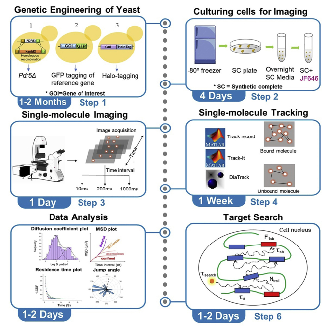
Single-molecule tracking (SMT) is a powerful approach to quantify the biophysical parameters of protein dynamics in live cells. Here, we describe a protocol for SMT in live cells of the budding yeast Saccharomyces cerevisiae. We detail how to genetically engineer yeast strains for SMT, how to set up image acquisition parameters, and how different software programs can be used to quantify a variety of biophysical parameters such as diffusion coefficient, residence time, bound fraction, jump angles, and target-search parameters.
For complete details on the use and execution of this protocol, please refer to Mehta et al. 1 and Ball et al..2
Subject areas: Single-molecule Assays, Cell Biology, Microscopy, Model Organisms
Graphical abstract
Highlights
-
•
Genetic engineering of yeast strains for single-molecule tracking
-
•
Strategies for single-molecule imaging and microscope setup
-
•
Tracking, data analysis, and data visualization using a variety of software packages
-
•
Estimation of residence time, bound fraction, diffusion coefficient, and target-search
Publisher’s note: Undertaking any experimental protocol requires adherence to local institutional guidelines for laboratory safety and ethics.
Single-molecule tracking (SMT) is a powerful approach to quantify the biophysical parameters of protein dynamics in live cells. Here, we describe a protocol for SMT in live cells of the budding yeast Saccharomyces cerevisiae. We detail how to genetically engineer yeast strains for SMT, how to set up image acquisition parameters, and how different software programs can be used to quantify a variety of biophysical parameters such as diffusion coefficient, residence time, bound fraction, jump angles, and target-search parameters.
Before you begin
-
1.
Order oligos for C-/N-terminal HaloTag and 3×GFP Tag integration to your genes of interest.
-
2.
Order plasmids for amplifying -HaloTag and 3×GFP Tag cassettes with selection markers (from Addgene).
-
3.
Order parental yeast strains (MATa and MATalpha, if you need diploid cells for your experiment).
-
4.
Order HaloTag ligands (HTL, JF646/JF549/JF552/TMR).
-
5.
For yeast transformation, streak parental yeast strains (from −80°C freezer) on a YPD plate to get the single colonies and incubate at 30°C for 2–3 days. Inoculate 1–2 colonies into 5 mL YPD tubes for yeast transformation.
Yeast media preparation
Timing: 2–3 h
Yeast culture media is required for growing yeast cells for yeast transformations and imaging. The YPD (yeast extract, peptone, dextrose) media is used only for the yeast transformations using the KANMX selection marker (antibiotic resistance marker), whereas Synthetic Complete (SC) media is used for yeast transformations using URA3 or TRP1 selection markers and for growing yeast cells to the log phase before single-molecule imaging. This section provides recipes for these media preparations.
-
6.YPD medium (100 mL).Note: YPD medium is used only for yeast transformation experiments for the genetic engineering of yeast strains using KANMX selection marker.
 CRITICAL: Don’t use YPD media for imaging experiments due to its autofluorescence.
-
a.Prepare the following two mixtures in two separate flasks of 250 mL.Mixture 1
Reagent Final concentration Amount Yeast extract 1% (w/v) 1 g Bacto peptone 2% (w/v) 2 g ddH2O N/A 50 mL Mixture 2Reagent Final concentration Amount D-(+)-Glucose 2% (w/v) 2 g Agar (only if solid media is required) 2% (w/v) 2 g ddH2O N/A 50 mL -
b.Autoclave both mixtures (at 121°C for 20 min).
-
c.Let both the mixtures cool down to ∼65°C, add mixture 1 to mixture 2, and stir well.
-
d.Add G418 antibiotic to 500 μg/mL concentration. Mix well.
-
e.If you need a liquid media, you can use it immediately after cooling down to 30°C. If you have added agar, pour the YPD media into 100 mm Petri dishes (∼25 mL media per petri dish).
-
a.
-
7.Synthetic Complete (SC) Media (100 mL).Note: Always grow yeast cells in the SC medium for single-molecule imaging experiments. For yeast transformations using URA3 or TRP1 selection marker, use SC-URA or SC-TRP media.
-
a.Prepare two mixtures in separate flasks.Mixture 1
Reagent Final concentration Amount YNB Powder 6.7 g/L 0.67 g Amino-Acid mixture (CSM/CSM-TRP/CSM-URA) 0.8 g/L 0.08 g ddH2O N/A 50 mL Mixture 2Reagent Final concentration Amount D-(+)-Glucose 2% (w/v) 2 g Agar (only if solid media is required) 2% (w/v) 2 g ddH2O N/A 50 mL -
b.Autoclave both mixtures (at 121°C for 20 min).
-
c.Let both the mixtures cool down to ∼65°C, add mixture 1 to mixture 2, and stir well.
-
d.If you need a liquid media, you can use it immediately after cooling down to 30°C. If you have added agar, pour the SC media into 100 mm Petri dishes (∼25 mL media per petri dish).
-
a.
Note: It is preferred to use aseptic conditions (Laminar Flow Hood) for pouring the plates, however, it is not mandatory. Under the laminar flow hood, the lid of the plates can be kept open for ∼45 min to remove excess moisture and the plates can be stored in a 4°C refrigerator for up to 6 months. For storage at 4°C, the plates should be placed in a plastic bag to prevent moisture loss. Liquid media can also be stored at 4°C and should be used within 15 days. Make sure to prewarm the liquid media and plates before use.
Note: For single-molecule imaging experiments, add 6.5 mg/mL sodium citrate to the SC media (liquid) for an improved signal-to-noise ratio.1
Note: The amino acid mixture is selected based on the strain genotype. CSM (Complete Supplement Mixture) powder contains all the amino acids, CSM-TRP contains all the amino acids except tryptophan, and CSM-URA contains all the amino acids except uracil.
Genetic engineering of yeast strains
For single-molecule tracking of a protein of interest in yeast S. cerevisiae, a minimum of three genetic manipulations are required: 1) deletion of a PDR5 gene: PDR5 gene codes for the membrane transporter protein Pdr5 that prevents the retention of xenobiotic compounds within the cell. For single-molecule imaging, we need fluorescent HaloTag Ligands (HTL, JF646-HTL/JF5552-HTL/JF549-HTL/TMR-HTL) to go inside the live cells to label our Protein Of Interest (POI). Yeast cells cannot retain these fluorescent ligands inside the cell, as Pdr5 exports them out of the cell. Hence, deletion of the PDR5 gene is essential to label the intracellular yeast proteins with fluorescent HTL.2 Deletion of PDR5 doesn’t affect the normal physiology of the cell and the cell growth remains unaffected.2 We can use the pdr5Δ yeast strain as a starting point for further genetic manipulation. 2) 3×GFP tagging of a localization marker/reference gene: to track the single-molecules of your POI within an organelle (e.g., nucleus, mitochondria etc.) or over the structures (such as spindles, transcription sites, replication sites etc.), you need to label such localization marker protein with 3×GFP. We preferably use histone H3 (HHT1) as localization marker for nucleus, TUB1 as a localization marker for spindles, transcription factor as a localization marker for transcription sites etc.). 3) C-/N- terminal Halo Tagging of the gene that codes for your POI. You should check the functionality of your POI after C-terminal Halo Tagging. Only if the functionality is compromised, you should go for the N-terminal Halo tagging. Generally, we use a PCR-based homologous recombination strategy for gene deletion and C-/N- terminal tagging.3,4 Below, we have provided detailed strategies for making these genetic manipulations.
Strategy for PDR5 gene deletion using KANMX6 as a selection marker:
To replace the endogenous PDR5 gene with the G418 (aminoglycoside antibiotic similar to kanamycin) resistance reporter gene (KANMX6).
-
8.
Amplify the KANMX6 cassette from the pUG6 vector (Euroscarf: P30114) using P101 and P102 primers (key resources table (KRT)). For PCR reaction set up, please refer.4
-
9.
Transform this PCR product into a parental haploid yeast strain and select the transformants on YPD Agar + 500 μg/mL G418. If using a diploid strain, it is required to delete PDR5 in both the haploids (MATa and MATalpha) to generate homozygous diploid. For yeast transformation protocol, please refer.4
-
10.
Verify the PDR5 gene deletion using a diagnostic PCR with primers P103 and P104 (KRT). Deletion of PDR5 provides an amplicon of 2,283 bp, whereas wild-type strain provides an amplicon of 5,209 bp.
Note: In diagnostic PCR using primers P103, P104, the wild-type PDR5 gene may not amplify any PCR product due to the long size of the amplicon (i.e., 5,209 bp). Either Taq polymerase fails to amplify such a long product, or the extension time (2–3 min) is not enough to allow complete amplification of this product. For further validation, one can design a forward primer from the KANMX gene (P105, KRT) to verify gene deletion using P105 and P104. PDR5 deletion produces a PCR amplicon of 997 bp, whereas wild-type PDR5 will not produce any PCR product. Alternatively, the deletion of PDR5 can be verified by Sanger sequencing.
Strategy for 3×GFP tagging of a reference gene/localization marker using URA3 as a selection marker:
-
11.
Amplify the 3×GFP-URA3 cassette from the pTSK405 vector (Addgene: 190817) using P106 and P107 primers (KRT). Please refer3 for C-/N- terminal tagging of a yeast gene.
-
12.
Transform this PCR product into a parental haploid yeast strain.
Note: For a diploid strain, if your protein is present at a higher concentration (e.g., histone (Hht1)), heterozygous 3×GFP tagging may work, however, if the protein abundance is low, then you may need homozygous 3×GFP tagging.
-
13.
Verify the labeling by fluorescence microscopy for GFP expression and localization.
Note: Make sure that the GFP signal is bright enough to see your entire structure (nucleus/transcription site/spindle/replication site) in a single-focal plane image. If you capture a 3D image (z-stack), you can see your structure in the maximum intensity projection (MIP) image, but in the single-focal plane image, you may not see it. In this case, choose a different localization marker that is more abundant to provide bright fluorescence.
Strategy for -Halo tagging of a Gene Of Interest (GOI) using URA3 or TRP1 as a selection marker:
-
14.
Amplify the -HaloTag-URA3 cassette from the pTSK561 vector (Addgene: 190816) using P108 and P109 primers (KRT). Alternatively, the HaloTag-TRP1 cassette can be amplified from the pTSK573 vector (Addgene: 190881) using P108 and P110 primers (KRT).
-
15.
Transform this PCR product into a parental haploid yeast strain. If using a diploid strain, it may work well if you tag only a single copy of your GOI with -HaloTag (heterozygous diploid).
-
16.
Verify the labeling by diagnostic PCR using gene-specific primers.
-
17.
You can also perform western blotting using Anti-HaloTag antibodies (KRT) to check the expression of the -Halo Tagged protein.
You can make additional genetic manipulations based on your experimental requirements, such as conditional depletion of proteins using auxin-induced degron or anchor-away technique, expression of a protein or deletion of a gene. Perform several functionality assays to make sure your protein remains functional after genetic manipulations. Make glycerol stocks of each of these strains and store them at −80°C freezer.
Key resources table
| REAGENT or RESOURCE | SOURCE | IDENTIFIER |
|---|---|---|
| Antibodies | ||
| Anti-HaloTag Monoclonal Antibody (Mouse) (1:1000 dilution) | Promega | Cat# G9211 RRID: AB_2688011 |
| Anti-HaloTag Polyclonal Antibody (Rabbit) (1:1000 dilution) | Promega | Cat# G9281 RRID: AB_713650 |
| Bacterial and virus strains | ||
| pUG6 | Euroscarf,4 | Euroscarf: P30114 |
| pTSK405 | Addgene,2 | Addgene: 190817 |
| pTSK561 | Addgene,2 | Addgene: 190816 |
| pTSK573 | Addgene,1 | Addgene: 190881 |
| Chemicals, peptides, and recombinant proteins | ||
| Janelia Fluor 646 (JF646)-HaloTag ligand | Promega | Cat# GA1120 |
| Janelia Fluor 552 (JF552)-HaloTag ligand | Grimm et al.5 | |
| Janelia Fluor 549 (JF549)-HaloTag ligand | Promega | Cat# GA1110 |
| TMR-HaloTag ligand | Promega | Cat# G8251 |
| Yeast Nitrogen Base (YNB) powder w/o Amino Acids, Carbohydrates & w/ AS | MP Biomedicals | Cat# 4027-522 |
| CSM-TRP | MP Biomedicals | Cat# 4511012 |
| CSM-URA | MP Biomedicals | Cat# 4511-212 |
| DOBA | MP Biomedicals | Cat# 4026-022 |
| BactoTM Agar | Thermo Fischer Scientific | Cat# 214030 |
| BactoTM Peptone | Thermo Fischer Scientific | Cat# 211677 |
| BactoTM Yeast Extract | Thermo Fischer Scientific | Cat# 288620 |
| D-(+)-Glucose | Sigma-Aldrich | Cat# 8270-1KG |
| G418 Sulfate | GoldBio | Cat# G-418-1 |
| SeaKem GTGTM Agarose | Lonza | 50070 |
| Deposited data | ||
| Example single-molecule imaging dataset for transcription factor Ace1-HaloTag-JF646 acquired with 200 ms time interval (30 ms exposure) | Mendeley Data1 | Mendeley Data: https://doi.org/10.17632/hp9bwtnbgc.1 |
| Experimental models: Organisms/strains | ||
| Yeast Saccharomyces cerevisiae haploids isogenic to S288C: BY4741, BY4742 | Euroscarf6 | Y00000, Y10000 |
| Oligonucleotides | ||
| Primer for PDR5 deletion using pUG6 (KANMX) (Forward) | AGACCCTTTTAAGTTTTCGT ATCCGCTCGTTCGAAAGAC TTTAGACAAAAGCCAGCTG AAGCTTCGTACG∗ |
P101 |
| Primer for PDR5 deletion using pUG6 (KANMX) (Reverse) | AAATTCAAGAAAATTGAAA TGTAGAAAGCTCGCTGAAT TAAGAAAAAAAAGGCCAC TAGTGGATCTG∗ |
P102 |
| Diagnostic primers for PDR5 deletion check (Forward) | CTCTTCTACGCCGTGGTACG | P103 |
| Diagnostic primers for PDR5 deletion check (Reverse) | GAAGACGGTTCGCCATTCG | P104 |
| Diagnostic primer for PDR5 deletion check from KANMX gene (Forward) | GCTGGCCTGTTGAACAAGTC | P105 |
| Primer for -3×GFP tag using pTSK405 (URA3) (Forward) | -50 bp gene specific sequences upstream of the STOP codon-CAAGCGGCCGCCGCTGCTGC∗ | P106 |
| Primer for -3×GFP tag using pTSK405 (URA3) (Reverse) | -Reverse complement 50 bp gene specific sequences downstream of the STOP codon (including STOP codon)- GCGT CCATCTTTACAGTCCT∗ |
P107 |
| Primer for -HaloTag using pTSK561/pTSK573 (URA3/TRP1) (Forward) | -50 bp gene specific sequences upstream of the STOP codon-CA AGCGGCCGCCGCTGCTGC∗ |
P108 |
| Primer for -HaloTag using pTSK561 (URA3) (Reverse) | -Reverse complement 50 bp gene specific sequences downstream of the STOP codon (including STOP codon)- GC GTCCATCTTTACAGTCCT∗ |
P109 |
| Primer for -HaloTag using pTSK573 (TRP1) (Reverse): | -Reverse complement 50 bp gene specific sequences downstream of the STOP codon (including STOP codon)-CTA TTTCTTAGCATTTTTGACG∗ |
P110 |
| Software and algorithms | ||
| ImageJ | Schneider et al.7 | https://imagej.nih.gov/ij/ |
| MatlabTrack v6.0 (MATLAB) | Ball et al.2 | https://sourceforge.net/projects/single-molecule-tracking |
| TrackIT (MATLAB) | Kuhn et al.8 | https://gitlab.com/GebhardtLab/TrackIt |
| Diatrack | Vallotton et al.9 | http://www.diatrack.org/index.html |
| Sojourner | Ranjan et al.10 | https://github.com/sheng-liu/sojourner |
| Spot-On | Hansen et al.11 | https://spoton.berkeley.edu/ |
| Other | ||
| LabTek II chambers, 2 well, 1.5 mm cover glass | Nunc | 155379 |
| Falcon 14 mL round bottom PP Test tube with snap cap | Falcon | Cat#352059 |
| Microwave oven with at least 800 W power | ||
| Orbital shaker with temperature control (230 RPM, 30°C) | Thermo Fisher Scientific | MaxQ 4000 |
| Single-Molecule Imaging Microscope (HILO illumination; 100× 1.49 NA TIRF objective lens; necessary hardware and software for simultaneous two colors fast imaging (with exposure time as low as 10 ms). | Olympus | IX83 |
| EMCCD camera: iXon Ultra 888 | Andor Technology | DU-888U-CS0-#BV |
| 488 nm (100 mW) laser | Coherent | OBIS 488LX |
| 647 nm (120 mW) laser | Coherent | OBIS 647LX |
| Tabletop centrifuge with 1.5 mL, 15 mL, 50 mL tube rotors | Eppendorf | 5804R |
| Vortex mixer | ||
∗Vector specific DNA sequences are shown in blue font.
Step-by-step method details
Culturing yeast cells for single-molecule imaging
For single-molecule imaging experiments, we need to revive the cells from the −80°C freezer, grow them to the log phase in SC media, and label the -HaloTag protein with HTL. Follow these steps for the same.
-
1.
Four days before imaging, streak yeast cells (from −80°C freezer) onto a SC+Agar plate to get single colonies. Incubate the plate at 30°C for 2 days.
-
2.
One day before imaging, inoculate a single colony in 3 mL SC broth (in 14 mL Falcon tube). Grow cells at 30°C at 230 RPM for 20–24 h for saturated growth.
-
3.
On the day of imaging, inoculate 50 μL of this saturated culture into a fresh 3 mL of SC media (in 14 mL Falcon tube). Grow cells at 30°C at 230 RPM for 4–5 h to bring them to the log phase of growth.
-
4.
Optional: If you want to give any treatment (e.g., auxin/rapamycin induction for protein depletion, induction for protein expression, etc.), add the inducer after 4 h of growth, keep it for shaking for another 1–2 h (depending on your experimental need) and then proceed.
-
5.
After 5 h growth, centrifuge 3 mL culture to pellet down the cells ( ∼ 541 × g for 1 min). Discard the supernatant and resuspend the cell pellet in 1 mL of fresh prewarmed SC media.
-
6.
Add fluorescently labeled HTL. Please refer to the note below for the selection of the HTL and its concentration.
Note: For single-molecule tracking, we need sparse labeling of the protein molecules so that their individual trajectories can be observed. Generally, we recommend labeling 3 to 5 molecules of protein per nucleus or 5–8 molecules of protein per cell. Such a low labeling density can be achieved by using an extremely low concentration of the HTL (Generally, JF646, JF552, JF549 or TMR work best with yeast). The labeling efficiency depends on the intracellular/intranuclear concentration of that protein. E.g., histone H3 (Hht1) is present in high abundance, so 0.005 nM JF646-HTL is enough to label 3 to 5 molecules per nucleus, whereas aurora kinase B (Ipl1) is present in low abundance, so 15 nM JF646-HTL is required to label 3 to 5 molecules per nucleus.
-
7.
Shake the culture for an additional 30 min after adding the HTL at 30°C at 230 RPM.
-
8.
Centrifuge the culture (541 × g for 1 min) to pellet down the cells. Discard the supernatant gently.
-
9.
Wash the cells twice or thrice with prewarmed SC media (1 mL each wash, 541 × g for 1 min) to remove unbound dye.
-
10.
Resuspend the cells in the remaining 10–20 μL of media. Take 3 μL of this cell suspension for imaging.
Note: We have observed an inverse relationship between the emission wavelength of the HaloTag ligand and cell permeability.12 The ligand with the higher emission wavelength (JF646) labels the HaloTag protein to the same extent at 100–1,000 times less concentration than the ligand with the shorter emission wavelength (JF549/TMR). Generally, the HaloTag ligands with a green fluorophore (JF503-HTL or JF525-HTL) fail to label the HaloTag proteins in yeast (Unpublished observation). Recently, Zheng et al. reported a similar observation that JF552-HTL show improved cell-permeability compared to JF549-HTL.13
Note: JF552 is more photostable with better signal-to-noise than JF646.10
Single-molecule imaging under the inverted microscope
For acquiring time-lapse single-molecule movies, live cells are placed under the nutrient agarose pad (8 mm × 8 mm) in a LabTekII chamber for a continuous supply of nutrients and to keep the cells in a monolayer (Figure 1). Cells are focused under the Highly Inclined and Laminated Optical (HILO) sheet microscope and time-lapse movies are acquired with below mentioned parameters.
Figure 1.

How to mount cells under the agarose pad for imaging
(A) LabTekII Imaging chamber with 3 μL of cell suspension.
(B) Agarose pad in petri dish, a piece of 8 × 8 mm has been removed using surgical blade.
(C) Agarose pad (8 × 8 mm) placed on the top of the cell suspension.
For making agarose pad, add 250 mg of SeaKem GTG Agarose to 25 mL of SC media in a 100 mL flask. Boil it in a microwave until all the agarose particles dissolve. Mix well and boil again. Pour exactly 15 mL media into a 100 mm Petri dish and let it solidify (∼20 min). Keep the lid of the petri dish open for 20 min to remove excess moisture. Prepare the agarose pad freshly (just before 1–2 h of imaging).
-
11.
Turn on the microscope software and hardware (camera, light source, lasers).
-
12.
Turn on the stage incubator at 30°C and leave it on for 30 min before imaging for temperature stabilization.
-
13.
Take LabTek II chamber with 1.5 mm cover glass.
-
14.
Put 3 μL of cell suspension from step no. 10 (Figure 1).
-
15.
Cut 8 mm × 8 mm agarose slab from the Petri dish using a surgical blade.
-
16.
Put this agarose slab upside down on top of the cell suspension (Figure 1).
-
17.
Gently press it with a finger or the back of a pipette tip to spread the cells evenly under the agarose pad and to arrange them in monolayer.
-
18.
Close the lid of the LabTek II chamber.
-
19.Focus on the cells under the microscope using a 100× 1.49 NA oil objective lens, in transmitted light mode.
-
a.Find out the best field for imaging.Note: Generally, we choose a field in which we get ∼10–20 cells in monolayer in the displayed image on the computer screen (not in the eyepiece, because the eyepiece has a bigger field of view than the camera).
-
b.After focusing, switch the transmitted light mode to fluorescence mode/reflected light mode.
-
a.
-
20.
Switch on the 488 laser to focus on the intracellular structure/protein labeled with GFP (e.g., nucleus/spindle/transcription site etc).
-
21.Set acquisition parameters in the imaging software as follows:
-
a.Excitation power: Start with 100 μW 488 nm laser, 1 mW 647 nm laser.
-
i.Adjust the power of the 488 nm laser such that the GFP-labelled protein/structure is clearly visible in the single-focal plane (see troubleshooting 1).
-
ii.Adjust the power of the 647 nm laser such that the single molecules of the -HaloTag protein are visible (Figure 2, see troubleshooting 2, 3).Note: Try to optimize the laser power so that the single-molecules are visible with sufficient signal to noise ratio (∼5:1) for automated detection, however, they should not be too bright as that will lead to fast photobleaching. While imaging with long exposure time, the laser power should be reduced proportionally.
-
i.
-
b.Exposure time:
-
i.Generally, 10–30 ms exposure time is recommended for quantifying the diffusion parameters (such as MSD, diffusion coefficient, a fraction of bound and unbound molecules, and target-search mechanism).
- ii.
-
i.
-
c.Z-stack: Generally, single-molecule tracking is performed from a single-focal plane time-lapse movie due to technical limitations, such as fast photobleaching of the single fluorophores and reduced speed of imaging. So, a z-stack is not mandatory. However, there are reports on single-molecule tracking in 3D.17,18,19
-
d.Time interval between frames: For single-molecule tracking, the images are acquired at different time intervals to extract different parameters.
-
i.Movies with continuous acquisition (10–30 ms exposure, 0 ms time lapse) are used to extract the diffusion parameters. However, continuous acquisition bleaches the fluorophores faster, so these movies are not good for quantifying the residence time because the residence time is curtailed due to photobleaching.
-
ii.For estimating the residence time, movies are acquired with a longer time-lapse. Generally, 100 ms, 200 ms, 500 ms, and 1,000 ms time intervals are recommended for yeast cells, as the movies collected with higher than 1,000 ms time intervals show cell movement and distortion of the tracks.
-
i.
-
e.Number of frames:
-
i.For continuous acquisition mode (10–30 ms exposure, 0 min time interval), it is recommended to capture ∼1,000–2,000 frames (until you see a negligible number of single molecules).
-
ii.For long time-lapse imaging (i.e., time interval 200 ms, 500 ms, 750 ms, 1,000 ms), acquire ∼200–400 frames (until you see a negligible number of single molecules).
-
i.
-
a.
-
22.
With this set of imaging parameters, acquire enough movies to get at least 1,000 tracks per strain or per condition.
Note: We generally have an imaging session of 4–5 h per day to collect 20 movies of each 0 ms time interval (1,000 frames), 200 ms time interval (200 frames), and 1,000 ms time interval (100 frames). We need ∼30 to 50 movies to get 1,000 tracks. So, 2–3 days of imaging (4–5 h daily) is required to complete one experiment (condition).
-
23.
Save all the movies as .tiff files.
Figure 2.

A field view of cells under GFP and 647 channels (single-focal plane images)
Select a field with ∼10–20 cell per image. Adjust the 488-laser power in such a way that the entire nucleus is visible in a single-focal plane. Adjust the 647laser power such that the single-molecules of Hht1 are visible with signal to noise ratio of at-least 5:1. Higher the laser power, faster the photobleaching. If residence time estimation is required, try not to bleach the single-molecules faster due to high laser power. Representative images have been shown with adequate labeling density, over labeling density and under labeling density. Yellow arrows show specific cells with over labeling and red arrows show specific cells with under labeling. Scale bar: 2 μm.
Expected outcomes
By following the steps 1–21, collect at-least 30–50 time-lapse movies and save them as .tiff files. Under optimized imaging conditions (as stated above), the images in both the channels (488 and 647 nm) should look like Figure 2 (adequate labeling). See the quantification and statistical analysis section below to learn image processing and data analysis to quantify the biophysical parameters such as residence time, bound fraction, jump distances, jump angles, and target-search parameters from these movies.
Quantification and statistical analysis
Image processing and tracking of single molecules
Several software packages are available for single-molecule tracking. Here, we show the interface of only three of the MATLAB based tracking software packages, MatlabTrack, TrackIt, and Diatrack. Ball et al.2 and Mehta et al.1 have used MatlabTrack for single-molecule tracking and quantifying the fraction of bound molecules, their residence times and target-search time. Ranjan et al.10 and Nguyen et al.15 have used Diatrack for single-molecule tracking, Sojourner for statistical analysis of single-molecule imaging data (to quantify mean squared displacements, diffusion coefficient, bound fraction, residence time, radius of confinement, jump angles, and target-search parameters) and Spot-On for the kinetic modeling of the single-molecule tracking data (to quantify diffusion coefficient and bound fraction). Kuhn et al.8 has used TrackIt for single-molecule tracking and quantifying the jump distances, jump angles, radius of confinement, diffusion coefficient, dissociation rate, and bound fraction.
To our experience, the MatlabTrack is quite user-friendly for residence time estimation, but it does not have many options for the diffusion parameters estimation and visualization. Some of the unique features of the MatlabTrack are the bandpass filtering of the images that makes the single molecules stand out from the noise (that makes automated tracking more accurate), multiple options to make custom ROIs (Region Of Interests), and options to edit, merge and delete tracks. The Diatrack is a user-friendly tracking software, but it doesn’t have options for ROI making and extended options for data analysis. So, the tracking data (x,y, and z position of particles with track information as .mat file) generated from the Diatrack needs to be channelized to the Sojourner for the statistical analysis of single-molecule trajectories for extracting diffusion parameters, residence time, and target-search parameters. As Diatrack do not offer an option for ROI making, we must create binary mask images using Fiji/Image J and apply it on the tracked data using Sojourner. Usage of Sojourner needs extensive knowledge of R programming and statistics. The .csv file generated from Sojourner (contains the x,y, and z positioning of particles with track information for all the movies) is uploaded on the Spot-On server for the two- or three- state kinetic modelling. By fitting the data to the jump distance histograms, the Spot-On provides values for the mean diffusion coefficient and bound fraction. The TrackIt is the most user-friendly software to extract the diffusion parameters (including jump distances, jump angels) and residence time with many single-click options for data visualization. So, readers can use any of these software packages depending on which kind of image dataset they have (whether they need to track molecules within custom made ROIs), what biophysical parameters they want to estimate and which kind of data visualization they are looking for.
Computer prerequisite
-
1.
Operating system: Windows 10 64-bit.
-
2.
MATLAB version 2017b and above needed to be pre-installed in the local computer.
-
3.
Download and install R. (R 3.3.0) (https://cran.r-project.org/bin/windows/base/).
-
4.
Download and install RStudio Desktop (https://www.rstudio.com/products/rstudio/download/).
Tracking package 1: MatlabTrack
Installation
Download MatlabTrack from (https://sourceforge.net/projects/single-molecule-tracking).
-
5.
Download and extract “MatlabTrack_v6.0.zip” to your “C:” drive.
-
6.
Open MATLAB.
-
7.
Click on “Set Path”, add MatlabTrack_v6.0 folder to the MATLAB path and select “Save” in the “Set path” panel.
Tracking
-
8.
Type “integratedTrackGui” in the MATLAB command window and press “Enter”. It should open the main Graphical User Interface (GUI) for tracking. This window shows several modules for image processing, particle detection, and tracking (Figure 3).
-
9.
First, press the “Load Stack” button to load a timelapse movie (.tiff file).
Note: Loading a movie may take a few seconds due to the larger file size. (The more the frames, the longer it takes to load). You can see the status at the right bottom corner of the GUI.
-
10.
Then set the data acquisition parameters by clicking on the “Set Parameters” button from the menu (next to the “File” menu). You must put the values for “Frame Time(s)” and “Pixel Size(μm)”. If the movie was acquired with a 200 ms time interval, then the Frame Time should be “0.2”. The pixel size on our microscope was “117” nm.
Note: You have to calculate the pixel size of your microscope, based on the camera pixel size and magnification. (Pixel size (nm)=camera pixel size (nm)/magnification(X)).
-
11.
To reduce noise from the images, use a computational filtering process.
Note: The MatlabTrack offers two types of filters for single particle identification: a band-pass filter and a LoG filter. The band-pass filter works best for our images. You are required to set the “Lower limit” and “Upper limit” for the filtering process. We usually set the two limits to 1 and 5 pixels, to track diffraction-limited spots with a pixel size of about 100 nm.
-
12.
This software offers an option to define the Region Of interest (ROIs) for tracking.
Note: The ROIs can be drawn manually, or you can use a standard size square/circle. Go to the standard ROI option and select the preferred shape (square/circle), adjust the desired diameter/area, and click “Done”. You can also open a reference image (generally an image from the GFP channel) to draw ROIs, based on the protein localization/structure visible in the GFP channel.
-
13.The “Find Peaks” module identifies the peak corresponding to single molecules.
-
a.For automated particle detection, adjust the intensity threshold so that the software identifies all the real particles in the filtered image, and does not or rarely detect any false particle. Generally, we set the “Threshold” value between 100–500.
-
b.For each of the identified peaks, the position of the centroid is calculated over a sub-image of size defined by the “window size” parameter (which we usually set to two pixels larger than the higher limit of the band-pass filter, i.e., 7). Also, checkmark the option “Fit PSF to the particles” which identifies the center of the diffraction-limited spots by fitting a 2D Gaussian to each of them.
-
c.Press the button “Find Particles” and wait for a while until the software detects particles in all the frames (it takes a few seconds, keep checking the status).
-
a.
-
14.
Quality check: after particle detection, check the detection of the particles in other frames by scrolling the bar left to right (below the image window).
-
15.
Once the particles are accurately identified, the tracking of the particles can be performed using the “Particle Tracking” module.
Note: This software offers two algorithms for particle tracking: 1) Nearest neighbor, 2) (LAP) uTrack. The nearest neighbor algorithm works best for our images. We set the following parameters: “Maximum” jumps: 6 pixels, “Shortest” track: 2 frames; “Gaps to” close: 4 frames.
-
16.
Click the “Track” button to track. It will take a few seconds. Check the status bar.
-
17.
After tracking has been completed, the tracks can be manually verified using “Check Tracks” under the “Manually Check Tracks” module. It will open a new window (Figure 4) with tools visualizing individual tracks and options for adding, deleting, and modifying the tracks individually.
Note: Some of the tracks do not need any manual editing (Figure 4B). Some of the tracks need editing/merging of small tracks (Figure 4C) and some of the tracks need to be deleted (Figure 4D). Look at the kymograph and see how the automated tracking (track line) overlaps with the real position of the particles for each track. For the tracks that do not overlap visually with the single-molecule spots in the kymograph, we delete those tracks. Press “Done” once you manually verify all the tracks. It will close this window and take you back to the previous window (integratedTrackGui).
-
18.
Press the “Preprocess Tracks” button for the analysis of tracks.
-
19.
Save the tracking information derived from the movie by clicking “Save Mat-Track file” under the “File” menu.
-
20.
Repeat this tracking process for all the movies acquired for a particular strain/condition. Make a separate folder at your convenient location to save all .mat files at one place.
Figure 3.

MatlabTrack GUI for single-molecule tracking
The various modules are bordered in red and numbered according to their sequence. 1. Press this button for loading the .tiff file (a time-lapse single-molecule movie), 2. Filter the images for denoising using Bandpass filter, 3. Create ROIs against your area of interest, where you want to track the single molecules (such as nucleus, spindle, transcription site visualized by GFP channel). A prompt will appear upon clicking “Add ROI” to load the reference image. 4. Detect particles using intensity thresholding, 5. Track the particles frame-to-frame to generate trajectories, 6. Manually check the tracks, delete, or edit, if necessary, 7. Analyze the tracks. Save the results as .mat file from the “File” menu.
Figure 4.

MatlabTrack GUI for manually verifying the tracks
(A) Using this window, you can visually verify the automated tracking performed by the software. You can also edit or delete or merge the tracks if required.
(B) Example of a track that do not need any manual editing.
(C) Example of tracks that we manually add and merge to make a single long track out of four short tracks.
(D) Example of tracks that we manually delete.
Analysis
-
21.
To analyze all the tracks together (obtained from multiple movies), go to the “Further Analysis” menu and click on “Merge and Analyze residence time (Mazza PB correction).” It will open a new window and ask for several prompts: Choose “Survival Time Distribution” (instead of “Residence Time Histogram”).
-
22.
Set the tracking parameters with respect to the corresponding frame-cycle-time of each movie. See the recommended parameters for different time intervals in Table 1.
-
23.
Select “All ROIs” for tracking.
-
24.
Click “Ok” and wait for a few minutes to get the survival time plot, photobleaching plot, and statistical analysis for the residence time calculation and fraction of bound molecules (Figure 5).
-
25.
Click on “Tools” menu in the “AnalyzeResTimes_GUI” window, select “Generate Pie Chart” to see the fraction of bound molecules with their residence time (Figure 5).
-
26.
Save this result from the “File” menu.
Table 1.
Tracking parameters for MatlabTrack
| Interval (ms) | Max frame to frame displacement | Nmin | Max end to end displacement |
|---|---|---|---|
| 15 | 0.31 | 22 | 0.73 |
| 200 | 0.43 | 6 | 0.61 |
| 500 | 0.47 | 4 | 0.65 |
| 1,000 | 0.55 | 4 | 0.67 |
Based on the time interval for imaging, appropriate tracking parameters needs to be filled in for merging data from all the movies and preparing the survival time distribution. We have quantified these parameters by tracking histone H3 (Hht1) in yeast S. cerevisiae.
Figure 5.

MatlabTrack GUI for analyzing survival time distribution
The left curve shows the photobleaching kinetics. The right curve shows the survival time distribution. You can checkmark the “Photobleaching Correction” box to normalize the survival time distribution with the photobleaching kinetics. Based on the fitting of the survival time distribution (either single exponential fit or double exponential fit), the fraction of bound molecules has been calculated as “f1”. The inverse of the koff value represents the residence time. Click on the “Tools” menu and select “Generate Pie Chart” option to see the fraction of bound molecules with their residence time. The “total tracks” (red rectangle) should be generally >1000 for better statistical significance.
Tracking package 2: TrackIt
Installation
-
27.
Download TrackIt from (https://gitlab.com/GebhardtLab/TrackIt).
-
28.
Unzip/extract the folder to your “C:” drive.
-
29.
From this folder, install the GRID toolbox (“GRID_for_trackit_v1_4.mltbx”).
-
30.
Open MATLAB.
-
31.
Drag the “TrackIt_v1_4.m” file to the editor window of the MATLAB.
-
32.
Run TrackIt by clicking the run button or (F5) from the MATLAB command line.
Tracking
-
33.
Add a movie file (.tiff file) via the “Movie selector” button in the movie panel (Figure 6).
-
34.
Load reference image (GFP channel) via the “Load 2nd movie/image” button.
-
35.
Select Gaussian filter (pixel 2) and Remove Background (20 pixel) for denoising of the reference image.
-
36.
Draw ROIs using the “Tracking-region” panel.
Note: Further region-specific classification of tracks can be done by creating sub-regions. These can either be drawn by hand or through an intensity threshold in the sub-regions panel.
-
37.
In the “Tracking” window, set the “Spot detection parameters” as follows:
Figure 6.

TrackIt GUI for single-molecule tracking
The various modules are bordered in red and numbered according to their sequence. 1. Press this button for loading the .tiff file(s) (a time-lapse single-molecule movie), 2. Load reference image(s) (GFP channel), 3. Filter the images for denoising, 4. Create ROIs against your area of interest, where you want to track the single molecules (such as nucleus, spindle, transcription site visualized by GFP channel), 5. Detect particles using intensity thresholding, 6. Track the particles frame-to-frame to generate trajectories, 7. Analyze movie. Save the results from the “File” menu using “Save batch file as” option.
Threshold factor: Threshold should be empirically determined for the accurate spot detection. Generally, we use a threshold value between “1–2”.
Frame range: Specifies the frames between which the spots should be detected and tracked. For tracking the entire movie (all the frames), use the values of “1” to “Inf (Infinite)”, but you can also remove a first few frames using this option.
Tracking parameters: Select an algorithm for tracking. Generally, in our images, the concentration of fluorescent molecules is low enough so that each spot is spatially well separated from others at all times. In this case the “nearest neighbor” algorithm delivers fast and reliable tracking results. For higher concentration, the u-Track algorithm may provide better results.
Tracking radius: Maximum distance (in pixels) at which spots are linked between two consecutive time points. Generally, we use “6” pixels.
Min. track length: Minimum number of frames a fluorescent molecule must persist to be accepted as a track. Generally, we use “2” frames.
Gap frames: Number of frames a fluorescent molecule may disappear or remain undetected, however, the tracking should be continued. Generally, we use “4” frames.2
Min. track length before gap frame: Number of frames a track must exist before closing of gaps (gap frames). Generally, we use “2” frames.
-
38.
Click on the “Analyze current movie” button to track single molecules.
-
39.
Go to “File” menu and click on “Save batch file as” to save the tracking data for one particular movie. Similarly, save the batch files for all other movies. These individual batch files can be further analyzed by loading them to the “Track explorer” GUI under the “Tools” menu.
-
40.
For merging all the individual batch files, go to “File” menu and select “Merge multiple batch files”. This merged batch file can be further analyzed by loading it to the “Tracking data analysis” GUI under the “Analysis” menu.
Analysis
-
41.
To analyze individual track, go to “Tools” menu and select “Track explorer”. It will open a new GUI with trajectory, kymograph, mean intensity, jump distance, MSD and jump angels (Figure 7).
-
42.
For analyzing batch file, go to “Analysis” menu and select “Tracking data analysis”. It will open a new GUI as shown in (Figure 8).
-
43.
To save these results, go to the “File” menu and press “Save” button and select your desired location to save this file.
Figure 7.

TrackIt Track explorer GUI for individual track analysis
This GUI shows each track (one at a time) with its trajectory, kymograph, mean intensity, jump distance, MSD, and jump angles.
Figure 8.

TrackIt GUI for batch data analysis
This GUI allows you to load all the batch files (.mat) of different strains/conditions for graphical visualization (panel 1). Panels 2 and 3 allows you to select different datasets/ROIs for graphical representation. Panels 4, 5, and 6 allows you to plot a variety of biophysical parameters or the track statistics.
Tracking package 3: Diatrack, Sojourner and Spot-On
Installation
Download and Install the Diatrack software (ver. 3.05, http://www.diatrack.org/index.html).
Tracking
Diatrack is used to localize the centroid of PSF (point spread function) by Gaussian fitting over the fluorescence intensity to sub-pixel resolution20,21 and single molecular tracking.22
-
44.
To perform single molecule tracking, upload the time-lapse movie (.tiff file) using the “Load image data” option under the “File” menu (Figure 9).
-
45.
Filter the image using Gaussian filter by pressing the button “Filter data”. The value should range between 0 to 1. Click the “Find particle” button to detect the particles.
-
46.
Press the button from the top panel (as shown by “2” in Figure 9) to activate the high precision mode. Set the Half Width at Half Maximum (HWHM) value to one pixel.
-
47.
For accurate particle selection, adjust the following parameters empirically: “Remove dim” and “Remove blurred”.
Note: Generally, for our images, we set the “Remove dim” to ∼“2,500” and “Remove blurred” to “0.1”. Set these two parameters in such a way that only the real particles are detected by the software (software shows “+” sign on the detected particles).
-
48.
Press “Process next frames” button to detect particles in rest of the frames.
-
49.
Press “Track!” button. It will show a prompt to set a “maximum particle jump in pixel?” Set this value to “6” for fast-tracking (15 ms time-interval) or ‘3’ for slow tracking (200 ms and 1,000 ms time interval). Diatrack uses a tripartite directed graph structure algorithm for tracking.9
-
50.
Save these tracking data as “.mat” file by selecting the “Save current session” under the “File” menu. This file contains information about the x, and y coordinates of the particles and the tracking information, which can be used for downstream analysis using Sojourner (see below).
Note: Diatrack does not provide an option to select the ROIs. However, to track the particles only in the defined area (i.e., nucleus), we create a mask image using ImageJ/Fiji and apply it to the next step of image analysis using Sojourner to filter out trajectories present outside the nucleus.
Figure 9.

Diatrack GUI for single-molecule tracking
Diatrack allows the detection and tracking of single molecules. Various modules are bordered red and numbered according to their sequence. Load the image from the “File” menu. 1. Filter the data using Gaussian filter, 2. Activate the High Precision mode for particle detection, 3. Find particles, 4 and 5. Deselect false particles by empirically adjusting “Remove dim” and “Remove blurred”, apply these selections to all the next frames by pressing the button “Process next frames”. 6. Track the particles by pressing “Track!” button to generate trajectories. Save the results from the “File” menu using “Save current session” option.
Data analysis pipeline by Sojourner
Sojourner is a R-based software for statistical analysis of single-molecule trajectories and data visualization (Ranjan et al.10). It is used for deriving biophysical metrics, such as mean squared displacement, diffusion coefficient, residence time and applying statistical analysis on the estimated metrics. The x and y coordinates of the particles and the tracking information can be imported to Sojourner from Diatrack for further processing.
Installation
-
51.
Open R Studio Desktop and enter:
if(!requireNamespace("BiocManager", quietly = TRUE))
install.packages("BiocManager")
BiocManager::install("sojourner")
Or install the Sojourner using the release version from GitHub:
devtools::install_github("sheng-liu/sojourner", build_vignettes = TRUE)
-
52.
Loading of sojourner package.
library(sojourner)
-
53.
The input file for Sojourner is the output file from Diatrack (.mat). Tracks are extracted from the Diatrack .mat file and then stored in a trackll, a list of track lists. A track denotes a single trajectory, recording x, y, z and frame number. Collection of track data output from one video file is designated as trackl. Similarly, a “trackll” is a collection of “trackl” in one folder.
setwd("/D:/Yeast SMT/Histone H3_15 ms interval")
Folder1="/D:/Yeast SMT/Histone H3_15 ms interval"
Track1<-createTrackll(folder=Folder1, input=2, cores=1, frameRecord=T)
Track1.fi<-filterTrack(trackll=Track1, filter=c(min=6,max=Inf))
-
54.
Sometimes a molecule will disappear for a number of frames due to photoblinking of the fluorescent dye, classifying one trajectory as two. Users can link trajectories that skip (or don’t exist for) a number of frames using the “linkSkippedFrames()” function.
Track1.fi.li<-linkSkippedFrames(trackll = Track1.fi,tolerance=2,maxSkip =5,cores=1)
-
55.
Use “maskTracks()” to add a binary image mask to the data being tracked. For each movie, we make a binary mask file using ImageJ based on the reference GFP channel image. Further to merge both mask image file and tracks we use the function “mergeTracks”.
mask.list=list.files(path=Folder1,pattern='_MASK.tif',full.names=TRUE)
Track1.fi.li.ma <- maskTracks(folder = Folder1, trackll = Track1.fi.li)
Track1.fi.li.ma.me<-mergeTracks(Folder1, Track1.fi.li.ma)
-
56.
To export a trackll file, use “exportTrackll()” function to save entire tracking data into a .csv file in the working directory.
exportTrackll(Track1.fi.li.ma.me)
-
57.
Calculate and plot the dwell times using the following script.
dwellTime(trackll=Track1.fi.li.ma.me,t.interval=15,x.scale=c(min=0,max=10000),output=TRUE, plot=TRUE)
-
58.
For estimating different biophysical properties of a molecule, e.g., mean square displacement (MSD), diffusion coefficient (Dcoef) etc., use the following script.
dcoef=Dcoef(trackll=Track1.fi.li.ma.me,dt=5,filter=c(min=6,max=Inf),method="static" , plot=T, output=T)
msd(Track1.fi.li.ma.me,dt=5, resolution=0.2, summarize=TRUE, cores=1,plot=TRUE, output=TRUE)
Kinetic modeling using Spot-On
Spot-On is a user-friendly web-interface that performs kinetic model-based analysis on the pooled single-molecule trajectories to produce the histograms of molecular displacements over time to estimate the fraction and diffusion constant of each subpopulation.11
-
59.
For Spot-On analysis, go to https://spoton.berkeley.edu/SPTGUI/, and click on “Start with my data set”.
-
60.
Upload the “.csv” file generated through Sojourner (step 13) using “Input format: MOSAIC suite” (Figure 10A).
-
61.
Provide values for “framerate (ms)” and “pixel size (nm/px)”. For our dataset, we use framerate of 15 ms and pixel size of 117 nm/px.
-
62.
It will populate the information regarding the loaded dataset under “Global statistics”.
-
63.
To perform kinetic modelling, go to the “Kinetic modelling” tab on the top panel.
-
64.
Fill the jump length distribution and (two state) model fitting parameters as shown in the Figures 10B and 10C. (These parameters can be selected empirically based on your data).
-
65.
Click on the “Fit kinetic model” button to perform the kinetic modelling.
-
66.
Wait for a few seconds to get the information about various fitting parameters such as Dbound (μm2/s), Dfree (μm2/s), and Fbound along with the jump length histograms.
Figure 10.

Spot-On interface for kinetic modeling of the SMT data
(A–C) (A) Upload .csv file (generated from Sojourner) as MOSAIC suite format and set the jump length distribution and model fitting parameters as shown (B and C) or empirically determine for your dataset. Press “Fit kinetic model” button to obtain the values for bound fractions and diffusion coefficients for each population.
Estimation of target-search parameters
By single-molecule tracking in live cells, one can estimate the target-search dynamics/parameters of a POI to understand how this protein finds its target binding site in the complex cellular environment. For detailed protocol, please refer.23 The following parameters can be quantified using the fast-tracking (short time interval, 0 ms) and the slow-tracking (long time interval, 200 ms, 500 ms, 750 ms, 1,000 ms) SMT data for a POI.
τsearch: target-search time is the time for locating a specific site.
Ntrial: average number of non-specific interactions before encountering the specific site.
τ3D: average free time between two binding events.
F1sb: specific-bound fraction at specific site.
τsb: residence time on specific site (specific binding).
τtb: residence time on nonspecific site (transient binding).
To determine the values of these parameters, process the fast-tracking SMT data through Spot-On to obtain F1, F2 and F3 (fraction of bound, slow/confined, and fast/free diffusion molecules, respectively).
Obtain the values for residence times τsb, τtb, and the stable and transient bound fractions (f1sb and f1tb) of total chromatin bound molecules by fitting the dwell-time distribution (after photobleaching correction) with a two-component decay function (using MatlabTrack). F1sb and F1tb, which are the stable and transient bound fractions of total proteins within cells, can be described as F1sb=F1 × f1sb and F1tb=F1 × f1tb, respectively.
The following equations can be used to calculate different target-search parameters.
| Ntrial=1/f1sb. |
| F1sb= τsb/(τsearch+τsb). |
| τsearch= Ntrial × τ3D + (Ntrial – 1) τtb. |
Limitations
Our efforts to label the intracellular yeast proteins with other self-labeling tags such as SNAP-Tag and CLIP-Tag were not successful. So, this protocol works best with -HaloTag and the HTL only.
The major limitation of single-molecule tracking is the photobleaching of the fluorescent dyes. The residence time estimations using single-molecule tracking are generally curtailed by photobleaching. So, this method is not accurate to measure the residence time of the immobile molecules (such as histones), however, it is the best method to measure the residence time of the fast-moving molecules/transient interactions (such as transcription factors). There are ways to do photobleaching corrections22,24 and photo blinking corrections,2 which improve residence time estimations, however, such corrections do not achieve the infinite residence time for the chromatin bound molecules such as histones. On a similar note, SMT of histones serve as a gold standard to define the upper/lower limits of the diffusion parameters (such as mean squared displacements, diffusion coefficient, bound fraction, jump distances, jump angels), however, its residence time estimation by SMT is always curtailed due to photobleaching.
Due to the photo blinking property of the fluorescent dyes (JF646/JF552/JF549/TMR), the automated tracking software breaks the long track into a few smaller tracks as and when blinking occurs. To circumvent this issue, Ball et al.2 have developed a correction procedure for photoblinking. By closing the gaps of 4 or fewer frames, better estimates for the residence time can be obtained under the same imaging conditions and using the same fluorophore.
Troubleshooting
Problem 1
As the single-molecule imaging is performed as a single-focal plane (not as z-stack) time-lapse movie, it is possible that the entire structure/organelle cannot be visualized by GFP in a single focal plane. E.g., if you want to track single molecules over the anaphase spindle (labelled by GFP-Tub1), you may not see the entire ∼6 μm long spindle in a single focal plane (step 19 in step-by-step method details).
Potential solution
Take 3D images of cells in 488 nm channel before and after capturing single-molecule time-lapse movies in 547 nm or 647 nm channels. If your structure is fast-moving (e.g., transcription site), you need simultaneous two-color imaging to capture the positions of the transcription site (under 488 nm channel) and single-molecules (under 552/647 nm channels). The transcription site may move out of focus (due to gene repositioning) during the period of the time-lapse movie, which may curtail the estimation of residence time. For quantifying the residence time of a transcription factor over the fast-moving transcription site, the best approach is the orbital tracking microscopy.25
Problem 2
While imaging yeast cells, you may see lot of autofluorescence in addition to the single-molecules in 549 or 647 nm channel (step 19 in step-by-step method details).
Potential solution
If the SC media components (YNB powder or CSM powder) are very old, it creates stress during cell growth and cells show too much autofluorescence. So, buy fresh YNB and CSM powders to avoid such autofluorescence.
Problem 3
While imaging in 646 or 549 nm channel for visualizing single-molecules, you may see either absence of single-molecules or bulk staining of your protein of interest (instead of single-molecules) (step 19 in step-by-step method details).
Potential solution
The absence of single-molecules suggests that your HTL concentration is too low, whereas bulk staining of your protein of interest suggest that your HTL concentration is too high. The labelling efficiency depends on the protein concentration, so proteins with high concentration (e.g., histones) need a very low concentration of HTL for sparse labeling, whereas proteins with low concentration (e.g., transcription factors) need higher concentration of HTL. While working with any protein for the first time, it is crucial to optimize the HTL concentration for sparse labeling of the molecules. In the first experiment, take 10-fold dilutions of the HTL (i.e., 5 nM, 0.5 nM, 0.05 nM, 0.005 nM) to see which dilution offers visualization of single-molecules, at-least in a few cells. Suppose you could see a few cells with single-molecules at 0.05 nM HTL concentration, then in the second experiment, take 2-fold dilutions of the HTL (within that range, i.e., 0.025 nM, 0.05 nM, 0.10 nM, 0.20 nM) to fine-tune the labeling density. Ideally, you should get 3–5 molecules labelled per nucleus, or 6–8 molecules labelled per cell. However, you may not find all the cells with the same labelling density. Typically, in a field of 20 cells, you may find 10 cells with single-molecules visualized, whereas, remaining 10 cells show bulk fluorescence. For tracking, only make ROIs for those cells which shows single-molecules from frame 1.
Resource availability
Lead contact
Further information and requests for resources and reagents should be directed to and will be fulfilled by the lead contact, Gunjan Mehta (gunjanmehta@bt.iith.ac.in).
Materials availability
The plasmids generated from this work (pTSK405, pTSK561, and pTSK573) are deposited to Addgene.
Acknowledgments
This work is supported by the Har-Govind Khorana Innovative Young Biotechnologist Award (BT/13/IYBA/2020/10) and the Ramalingaswami Fellowship (BT/RLF/Re-entry/53/2020) to G.M. from the Department of Biotechnology, Govt. of India. We acknowledge the seed grant from IIT Hyderabad to G.M. N.K.P. and P.D. acknowledge the Prime Minister’s Research Fellowship for the financial support. We are grateful to Dr. Anand Ranjan (at Carl Wu’s Lab at John Hopkins University, Baltimore, USA) for guiding us through the data analysis pipeline using Diatrack, Sojourner, and Spot-On.
Author contributions
Methodology, N.K.P., A.D., G.M.; Software, N.K.P., A.D.; Validation, N.K.P., A.D., P.D., S.P.; Visualization, N.K.P., A.D., G.M.; Data curation, N.K.P., A.D., G.M.; Writing-Original draft preparation, N.K.P., A.D., G.M.; Writing-Reviewing and Editing, N.K.P., A.D., P.D., S.P., G.M.; Conceptualization, G.M.; Investigation, G.M.; Resources, G.M.; Supervision, G.M.; Project administration, G.M.; Funding acquisition, G.M.
Declaration of interests
The authors declare no competing interests.
Data and code availability
This study did not generate datasets.
References
- 1.Mehta G.D., Ball D.A., Eriksson P.R., Chereji R.V., Clark D.J., McNally J.G., Karpova T.S. Single-molecule analysis reveals linked cycles of RSC chromatin remodeling and Ace1p transcription factor binding in yeast. Mol. Cell. 2018;72:875–887.e9. doi: 10.1016/j.molcel.2018.09.009. [DOI] [PMC free article] [PubMed] [Google Scholar]
- 2.Ball D.A., Mehta G.D., Salomon-Kent R., Mazza D., Morisaki T., Mueller F., McNally J.G., Karpova T.S. Single molecule tracking of Ace1p in Saccharomyces cerevisiae defines a characteristic residence time for non-specific interactions of transcription factors with chromatin. Nucleic Acids Res. 2016;44:e160. doi: 10.1093/nar/gkw744. [DOI] [PMC free article] [PubMed] [Google Scholar]
- 3.Janke C., Magiera M.M., Rathfelder N., Taxis C., Reber S., Maekawa H., Moreno-Borchart A., Doenges G., Schwob E., Schiebel E., Knop M. A versatile toolbox for PCR-based tagging of yeast genes: new fluorescent proteins, more markers and promoter substitution cassettes. Yeast. 2004;21:947–962. doi: 10.1002/yea.1142. [DOI] [PubMed] [Google Scholar]
- 4.Güldener U., Heck S., Fielder T., Beinhauer J., Hegemann J.H. A new efficient gene disruption cassette for repeated use in budding yeast. Nucleic Acids Res. 1996;24:2519–2524. doi: 10.1093/nar/24.13.2519. [DOI] [PMC free article] [PubMed] [Google Scholar]
- 5.Grimm J.B., Tkachuk A.N., Xie L., Choi H., Mohar B., Falco N., Schaefer K., Patel R., Zheng Q., Liu Z., et al. A general method to optimize and functionalize red-shifted rhodamine dyes. Nat. Methods. 2020;17:815–821. doi: 10.1038/s41592-020-0909-6. [DOI] [PMC free article] [PubMed] [Google Scholar]
- 6.Baker Brachmann C., Davies A., Cost G.J., Caputo E., Li J., Hieter P., Boeke J.D. Designer deletion strains derived from Saccharomyces cerevisiae S288C: a useful set of strains and plasmids for PCR-mediated gene disruption and other applications. Yeast. 1998;14:115–132. doi: 10.1002/(SICI)1097-0061(19980130)14:2<115::AID-YEA204>3.0.CO;2-2. [DOI] [PubMed] [Google Scholar]
- 7.Schneider C.A., Rasband W.S., Eliceiri K.W. NIH Image to ImageJ: 25 years of image analysis. Nat. Methods. 2012;9:671–675. doi: 10.1038/nmeth.2089. [DOI] [PMC free article] [PubMed] [Google Scholar]
- 8.Kuhn T., Hettich J., Davtyan R., Gebhardt J.C.M. Single molecule tracking and analysis framework including theory-predicted parameter settings. Sci. Rep. 2021;11:9465. doi: 10.1038/s41598-021-88802-7. [DOI] [PMC free article] [PubMed] [Google Scholar]
- 9.Vallotton P., van Oijen A.M., Whitchurch C.B., Gelfand V., Yeo L., Tsiavaliaris G., Heinrich S., Dultz E., Weis K., Grünwald D. Diatrack particle tracking software: review of applications and performance evaluation. Traffic. 2017;18:840–852. doi: 10.1111/tra.12530. [DOI] [PMC free article] [PubMed] [Google Scholar]
- 10.Ranjan A., Nguyen V.Q., Liu S., Wisniewski J., Kim J.M., Tang X., Mizuguchi G., Elalaoui E., Nickels T.J., Jou V., et al. Live-cell single particle imaging reveals the role of RNA polymerase II in histone H2A. Elife. 2020;9:e55667. doi: 10.7554/eLife.55667. [DOI] [PMC free article] [PubMed] [Google Scholar]
- 11.Hansen A.S., Woringer M., Grimm J.B., Lavis L.D., Tjian R., Darzacq X. Robust model-based analysis of single-particle tracking experiments with Spot-On. Elife. 2018;7:e33125. doi: 10.7554/eLife.33125. [DOI] [PMC free article] [PubMed] [Google Scholar]
- 12.Podh N.K., Paliwal S., Dey P., Das A., Morjaria S., Mehta G. In-vivo single-molecule imaging in yeast: applications and challenges. J. Mol. Biol. 2021;433:167250. doi: 10.1016/j.jmb.2021.167250. [DOI] [PubMed] [Google Scholar]
- 13.Zheng Q., Ayala A.X., Chung I., Weigel A.V., Ranjan A., Falco N., Grimm J.B., Tkachuk A.N., Wu C., Lippincott-Schwartz J., et al. Rational design of fluorogenic and spontaneously blinking labels for super-resolution imaging. ACS Cent. Sci. 2019;5:1602–1613. doi: 10.1021/acscentsci.9b00676. [DOI] [PMC free article] [PubMed] [Google Scholar]
- 14.Kapadia N., El-Hajj Z.W., Reyes-Lamothe R. Bound2Learn: a machine learning approach for classification of DNA-bound proteins from single-molecule tracking experiments. Nucleic Acids Res. 2021;49:e79. doi: 10.1093/nar/gkab186. [DOI] [PMC free article] [PubMed] [Google Scholar]
- 15.Nguyen V.Q., Ranjan A., Liu S., Tang X., Ling Y.H., Wisniewski J., Mizuguchi G., Li K.Y., Jou V., Zheng Q., et al. Spatiotemporal coordination of transcription preinitiation complex assembly in live cells. Mol. Cell. 2021;81:3560–3575.e6. doi: 10.1016/j.molcel.2021.07.022. [DOI] [PMC free article] [PubMed] [Google Scholar]
- 16.Kapadia N., El-Hajj Z.W., Zheng H., Beattie T.R., Yu A., Reyes-Lamothe R. Processive activity of replicative DNA polymerases in the replisome of live eukaryotic cells. Mol. Cell. 2020;80:114–126.e8. doi: 10.1016/j.molcel.2020.08.014. [DOI] [PubMed] [Google Scholar]
- 17.Hou S., Johnson C., Welsher K. Real-time 3D single particle tracking: towards active feedback single molecule spectroscopy in live cells. Molecules. 2019;24:2826. doi: 10.3390/molecules24152826. [DOI] [PMC free article] [PubMed] [Google Scholar]
- 18.Thompson M.A., Casolari J.M., Badieirostami M., Brown P.O., Moerner W.E. Three-dimensional tracking of single mRNA particles in Saccharomyces cerevisiae using a double-helix point spread function. Proc. Natl. Acad. Sci. USA. 2010;107:17864–17871. doi: 10.1073/pnas.1012868107. [DOI] [PMC free article] [PubMed] [Google Scholar]
- 19.Ram S., Kim D., Ober R.J., Ward E.S. 3D single molecule tracking with multifocal plane microscopy reveals rapid intercellular transferrin transport at epithelial cell barriers. Biophys. J. 2012;103:1594–1603. doi: 10.1016/j.bpj.2012.08.054. [DOI] [PMC free article] [PubMed] [Google Scholar]
- 20.Thompson R.E., Larson D.R., Webb W.W. Precise nanometer localization analysis for individual fluorescent probes. Biophys. J. 2002;82:2775–2783. doi: 10.1016/S0006-3495(02)75618-X. [DOI] [PMC free article] [PubMed] [Google Scholar]
- 21.Yildiz A., Forkey J.N., McKinney S.A., Ha T., Goldman Y.E., Selvin P.R. Myosin V Walks hand-over-hand: single fluorophore imaging with 1.5-nm localization. Science. 2003;300:2061–2065. doi: 10.1126/science.1084398. [DOI] [PubMed] [Google Scholar]
- 22.Vallotton P., Olivier S. Tri-track: free software for large-scale particle tracking. Microsc. Microanal. 2013;19:451–460. doi: 10.1017/S1431927612014328. [DOI] [PubMed] [Google Scholar]
- 23.Brown K., Kent S., Ren X. Quantifying the global binding and target-search dynamics of epigenetic regulatory factors using live-cell single-molecule tracking. STAR Protoc. 2021;2:100959. doi: 10.1016/j.xpro.2021.100959. [DOI] [PMC free article] [PubMed] [Google Scholar]
- 24.Garcia D.A., Fettweis G., Presman D.M., Paakinaho V., Jarzynski C., Upadhyaya A., Hager G.L. Power-law behavior of transcription factor dynamics at the single-molecule level implies a continuum affinity model. Nucleic Acids Res. 2021;49:6605–6620. doi: 10.1093/nar/gkab072. [DOI] [PMC free article] [PubMed] [Google Scholar]
- 25.Donovan B.T., Huynh A., Ball D.A., Patel H.P., Poirier M.G., Larson D.R., Ferguson M.L., Lenstra T.L. Live-cell imaging reveals the interplay between transcription factors, nucleosomes, and bursting. EMBO J. 2019;38:e100809. doi: 10.15252/embj.2018100809. [DOI] [PMC free article] [PubMed] [Google Scholar]
Associated Data
This section collects any data citations, data availability statements, or supplementary materials included in this article.
Data Availability Statement
This study did not generate datasets.