An income equalisation policy and social welfare: beyond inequality

Abstract

The inequality of income distribution is one of the most serious problems to our society. Traditional economics proposes the tax increase on wealthy classes and transfers its revenue to low income group. This is the most appropriate one. But, the total of this and donation will unfortunately be insufficient. For procuring funds to ease inequality, I propose to erase the government bonds which are already purchased and owned by the central bank. The government, then, issues new government bonds (the total sum of which should be less than erased one) to expend for equalization. The amount of new government bonds is determined from the maximisation of social welfare function concerning to income distribution. By this policy, first, the socially optimal equalization will be attained; second, through the productivity increase caused by the expenditure for low income group, the national economy will grow; third, because of the erasure process, the government bonds outstanding will not increase. In these days of pandemic, much more government expenditures are needed and thereby government deficits are piled up. I think the valid policy is not the heavy tax increase, but the execution of erasure of government bonds outstanding and to equalize income distribution.

Introduction

In the history of humankind, political and economic inequalities have always coexisted. At the end of the eighteenth century, the citizen’s revolution alleviated political inequality, which gradually spread across the globe. After the end of absolutism and advent of the industrial revolution, people expected economic equality and the prosperity of ordinary workers, and considerable effort was spent to achieve it. However, economic inequality still exists. Economic society can resolve the problem of inequality of income and properties.

Economics is an effective discipline having a wide range. The study on the allocation and distribution of scarce resources is an important field. The studies on resource allocation have obtained excellent results, but the studies on distribution have not achieved the desired results despite the strenuous efforts of economists. To rectify income and property inequality, economics mainly proposes tax increases or the increase of the rate of progressive tax. This is the most appropriate and authentic measure that has successfully reduced inequality. However, inequality still persists and the policy of tax increase cannot solely resolve the ongoing inequality. As the tax increase policy faces the strong political and economic oppositions and, moreover, has an upper limit, the inequality problem will exist semi-permanently.

In this study, a new policy is proposed that can resolve the problem of economic inequality. This policy suggests discontinuing the existing government bonds with the central bank, and then issuing new government bonds to expend for income equalisation. The amount of new issue will be less than the discontinued sum and will be determined from the standpoint of social welfare maximisation. The process of erasure and expense is devised to repeat at a declining rate. By this policy, the income distribution approaches the socially optimal point. The expenditure for income equalisation will increase people’s income which in turn will increase the tax revenue, thereby reducing the government deficit.

This study proposes an alternative to the existing policy of progressive taxation for reducing income inequality. I believe that this study makes contribution to the literature because it discusses in detail the erasure policy that can accomplish absolute income equality which the traditional tax policy has not realized.

As this erasure policy faces the problems of inflation and lax financial policy, close attention and deliberate countermeasures are indispensable.

The causes of present inequality

The inequality pressure from outside

The prevalence of the market economy in most parts of the world led to the acceptance of direct investment and the newest technology by developing countries, which enabled these countries to produce high-quality goods with low costs along with low wage rates, low rent, and diligence. They export these goods to industrialised countries. Thus, both sets of countries benefit from international trade.

However, the domestic firms of industrialised countries must compete with the imports that are of high quality and low price; otherwise, employment and the general wage rate will decrease. As a result of globalization and economic liberalization, the people of developing countries move to high-wage countries. This is advantageous to firms of industrialised countries but disadvantageous to workers who have been employed on high wages. The income of middle class workers who stably supported society has considerably decreased, resulting in a dwindling middle class.

The inequality pressure from inside

Currently, many start-ups have been founded in the fields of Internet of Things (IoT), artificial intelligence, biotechnology, and others. Some of them have grown into worldwide enterprises which have de facto standards. These enterprises supply goods and services which enhance the productivity of economy tremendously and therefore become the indispensable items for society to progress. These high-quality goods are improved continuously, and the real price of these have a tendency to decline. This also contributes towards the economy. The founders, investors, and entrepreneurs of these companies gain enormous income and wealth as a reward. These innovative enterprises usher changes to the traditional old-fashioned companies and in some cases induce withdrawal or bankruptcy. This leads to the increase in company efficiency; however, it also increases the number of unemployed people and decreases wages. Most of the rising innovative enterprises are fabless and outsource production to foreign manufacturers, leading to a decrease in domestic employment. Thus, a rise in innovative enterprises causes income disparity as a few successful persons become extremely rich; however, workers’ average income decreases gradually, and at worst, causes a rise in unemployment.

The COVID-19 pandemic

The recent COVID-19 pandemic has aggravated the unequal distribution of income. To prevent the spread of the pandemic, many countries declared a state of emergency, affecting international as well as domestic economies. Numerous workers lost their jobs. The benefits provided by the government to the workers have not been enough. Low- or middle-income patients suffering from the long-term symptoms of the pandemic often lose the ability to work. The disparities between the wealthy and unemployed or sick people are increasing, leading to an increase in the government deficit. Many economists insist that tax increases are inevitable to restore the soundness of the government budget.

Literatures on inequality

Market economy and democracy have historically overcome many obstacles. There are various distinguished contributions to the analysis of inequality. In the era, the bourgeoisie was on the rise, Adam Smith (1776) formulated the significant concept that through the working of the market mechanism (and the adoption of the division of labour system), the capitalist class, the land-owing class, and the working class can live harmoniously. This concept conveys that the market economy does not bring about severe inequality. But reality contradicts this. Workers’ long-lasting struggles to fight inequality still continue. Pigou (1920) founded the welfare economics and in it he insisted that equalisation of national dividend (or national income) will, ceteris paribus, increase the economic welfare. After his analysis, welfare analysis on income distribution developed.1 Seeing the unprecedented massive unemployment caused by the Great Depression (started from 1929), Keynes (1936) had a doubt about the effectiveness of neoclassical economics2 to solve it. Massive unemployment is one of the most serious threats to the society and to the income inequality.3 He founded the macroeconomics. In it he affirmatively evaluated the activities of entrepreneurs and workers, and placed low value on the activities of the people who does not contribute to production. A representative example of the latter is the rentier. Keynes considered that the rentiers did not contribute to the recovery of Britain’s economy at that time. Kuznets (1955) examined economic growth and income distribution. The ‘Kuznets Curve’ has been one of the bases of inequality analysis. Although Friedman (1962) believed in the efficient working of the market, he did not fail to notice the inequality of income and property. He advanced the system of negative income tax and mentioned that the determination of the minimum income level of this system depends on the sum the society can subsidize. He was also sensitive towards the inequality brought about by the market. Sen (1973; 1982) insisted that both utility level and the level of basic goods are not appropriate for measuring welfare. Instead, he proposed the concept “basic capability4” and used it to revise inequality. Atkinson’s empirical studies (1975; 1987; 20115) elucidate and tackle the inequality problem. He also published a book (2015) that proposed practical policies to rectify inequality. Deaton’s approach (2013) involves the relationship between health and wealth, and turns attention towards people of developing countries. Piketty’s studies (20036; 2014) cover a long span and criticize Kuznets’ findings, stirring debates and reinforcing people’s interest. Regarding the policy prescription for income equalisation, Friedman’s concept (1969) of ‘helicopter money’ can be applicable to the problems of inequality as well as deflation. Modern monetary theory (MMT) proposed by Wray (2015) and Kelton (2020) among others, presents a new way of understanding public finance and monetary theory. This theory observed the behaviour of the Bank of Japan (BOJ; central bank) and financial market. A government’s budget deficit is not the reason to revise unequal income distribution. Ravallion (2016) made an intensive study on the economic inequality.

The study is structured as follows: the contents of the policy are explained in (“Economic growth and social welfare”, “Erasure of government bonds”, “The pandemic and income equalisation”, “Apprehension regarding inflation” and “The effectiveness of income equalizing expenditure R”). The next section elucidates (“Traditional measures of equalisation”), and the subsequent section describes the (“Multiplier analysis”). (“Concluding remarks”) concludes the paper.

Economic growth and social welfare

Social welfare function concerning income distribution

This study presents a normative analysis of the relationship between economic growth and income inequality. The variables of this model are those of macroeconomics. The social welfare function developed by Bergson (1938) and Samuelson (1947) is applied to consider the problem. From the standpoint of economic policy, this function is maximised, and the method of analysis is that of microeconomics. Therefore, this model is developed by the combination of macroeconomics and microeconomics.

The national income of a country is denoted as $Y$, and is assumed to be composed of labour income $\mathit{wL}$ (where $w$: wage rate, $L$: labour), capital income $\mathit{rK}$ ($r$: interest rate, $K$: capital), and entrepreneurs’ income or profit, $\mathrm{\Pi }$, i.e. $Y=wL+rK+\mathrm{\Pi }$. The national income $Y$ is divided into two parts: labour income $\mathit{wL}$ denoted as $Y_L$; and the sum of capital income $\mathit{rK}$ and entrepreneurs’ income (profit) $\mathrm{\Pi }$, termed as property income and denoted as $Y_P$. That is:

$$\left\{\begin{array}{c}\begin{array}{c}Y\\ \left(\text{National}\text{income}\right)\end{array}\begin{array}{c}=\\ =\end{array}\begin{array}{c}\mathit{wL}\\ \left(\text{Labour}\text{income}\right)\end{array}\begin{array}{c}+\\ +\end{array}\begin{array}{c}\mathit{rK}\\ \left(\text{Capital}\text{income}\right)\end{array}\begin{array}{c}+\\ +\end{array}\begin{array}{c}\mathrm{\Pi }\\ \begin{array}{c}\left(\text{Entrepreneurs'}\text{income}\right)\\ \left(\text{profit}\right)\\ \end{array}\end{array}\\ \begin{array}{c}Y\\ \left(\text{National}\text{income}\right)\end{array}\begin{array}{c}=\\ =\end{array}\begin{array}{c}{Y}_L\\ \left(\text{Labour}\text{income}\right)\end{array}\begin{array}{c}+\\ +\end{array}\begin{array}{c}{Y}_P\\ \left(\text{Property}\text{income}\right)\end{array}\\ \end{array}\right)$$ 1

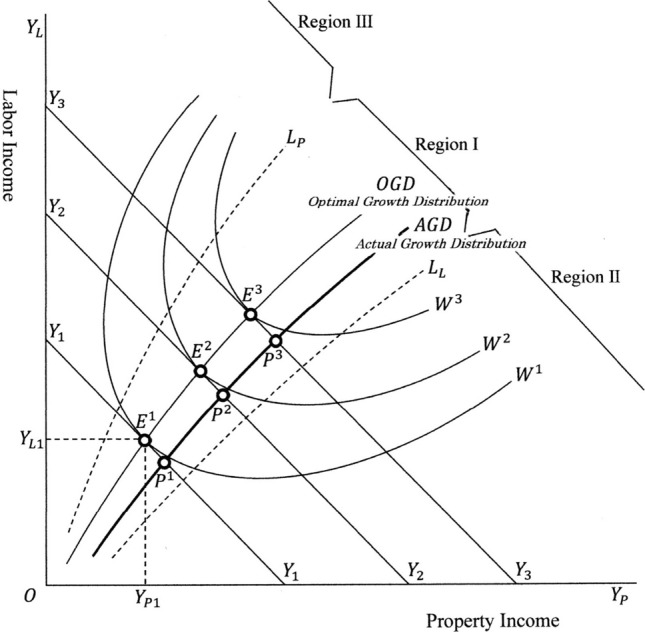
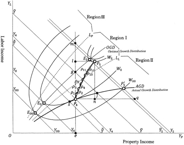
This is illustrated in Fig. 1, where the labour income $Y_L$ is measured along the vertical axis and property income $Y_P$ along the horizontal axis. The national income $Y$ is depicted as lines, $Y_1{Y}_1,Y_2{Y}_2,$ $Y_3{Y}_3,\cdots$, according to the income level $Y_1,Y_2,Y_3,\cdots$. The line $Y_i{Y}_i(i=1,2,3,\cdots )$ is called the ‘national income line’. The slope of this line is − 45°, and it shifts above to the right as the economy (national income) grows.

Fig. 1.

Socially equal distribution

The workers’ utility from labour income $Y_L$ is denoted as $u_L\left(Y_L\right)$, and capital owners’ and entrepreneurs’ utility from property income $Y_P$ is denoted as $u_P(Y_P)$. Then, the social welfare function $W$ concerning income distribution is formulated as:

$$W=W\left(u_L\left(Y_L\right),u_P\left(Y_P\right)\right)$$ 2

The social (welfare) indifference curves concerning income distribution are derived from (2), and depicted as $W^1,W^2,W^3$ in Fig. 1. As to the relative height of the utility, it is assumed that inequality $W^1<W^2<W^3$ holds. The slope of these curves is shown as:

$$\frac{d{Y}_L}{d{Y}_P}=-\frac{\left(\partial W/\partial u_P\right)\left(\partial u_P/\partial Y_P\right)}{\left(\partial W/\partial u_L\right)\left(\partial u_L/\partial Y_L\right)}.$$ 3

If social welfare (2) is maximised subject to the income distribution constraint (1), the optimal conditions are derived as:

$$\frac{\partial W}{\partial u_L}\frac{\partial u_L}{\partial Y_L}=-\lambda ,\frac{\partial W}{\partial u_P}\frac{\partial u_P}{\partial Y_P}=-\lambda ,Y_L+Y_P=Y$$ 4

The conditions (4) are the points of contact of the national income lines with social indifference curves and are shown as $E^1,E^2,E^3$. As national income $Y$ increases, or as the economy grows, the point of contact moves above to the right, and the path is depicted as the optimal growth distribution ($OGD)$. The locus of this curve is shown as:

$$\left\{\begin{array}{c}\frac{d{Y}_L}{\mathit{dY}}=\frac{W_{\mathit{LP}}{u}_P^{{}^{\prime }}{u}_L^{{}^{\prime }}-\left(W_{\mathit{PP}}{\left(u_P^{{}^{\prime }}\right)}^2+W_P{u}_P^{{}^{″}}\right)}{\mathrm{\Delta }}\\ \frac{d{Y}_P}{\mathit{dY}}=\frac{W_{\mathit{PL}}{u}_P^{{}^{\prime }}{u}_L^{{}^{\prime }}-(W_{\mathit{LL}}{(u_L^{{}^{\prime }})}^2+W_L{u}_L^{{}^{″}})}{\mathrm{\Delta }}\\ \end{array}\right)$$ 5

where $W_L=\partial W/\partial u_L,W_P=\partial W/\partial u_P,W_{\mathit{LP}}={\partial }^{2}W/\partial u_P\partial u_L,W_{\mathit{PL}}={\partial }^{2}W/\partial u_L\partial u_P,$ $W_{\mathit{LL}}={\partial }^{2}W/\partial u_L^2,W_{\mathit{PP}}={\partial }^{2}W/\partial u_P^2,u_L^{{}^{\prime }}=\partial u_L/\partial Y_L,u_P^{{}^{\prime }}=\partial u_P/\partial Y_P,u_L^{{}^{″}}={\partial }^2{u}_L/\partial Y_L^2,u_P^{{}^{″}}={\partial }^2{u}_P/\partial Y_P^2$ and$\mathrm{\Delta }=W_{\mathit{LP}}{u}_L^{{}^{\prime }}{u}_P^{{}^{\prime }}+W_{\mathit{PL}}{u}_P^{{}^{\prime }}{u}_L^{{}^{\prime }}-\left[W_{\mathit{LL}}{\left(u_L^{{}^{\prime }}\right)}^2+W_L{u}_L^{{}^{″}}\right)\left(+W_{\mathit{PP}}{\left(u_P^{{}^{\prime }}\right)}^2+W_P{u}_P^{{}^{″}}\right]>0$.7 Equation (5) shows the social optimal economic growth-income distribution curve $\mathit{OGD}$, which represents the locus of socially optimal income distribution when the economy grows.

On both sides of this $\mathit{OGD}$ curve, the socially permissible border lines regarding income inequality are depicted. The border line of the minimum permissible labour income, from the standpoint of social welfare, is depicted as $L_L$ in Fig. 1, and the property income is depicted as $L_P$.

Regarding the slope of social welfare indifference curves (3), the sign of terms $\partial u_L/\partial Y_L$ and $\partial u_P/\partial Y_P$ is assumed to be positive. The sign of terms $\partial W/\partial u_L$ and $\partial W/\partial u_P$ must be examined. Three regions are classified:

$$\left\{\begin{array}{c}\text{Region}\text{I: region}\text{between}\text{the}{\text{L}}_L\text{line}\text{and}{\text{L}}_P\text{line}\\ \partial W/\partial u_L>0,\partial W/\partial u_P>0\\ \text{Region}\text{II: region}\text{right}\text{to}\text{the}\text{line}{\text{L}}_{\text{L}}\\ \partial W/\partial u_L>0,\partial W/\partial u_P<0\\ \text{Region}\text{III: region}\text{left}\text{to}\text{the}\text{line}{\text{L}}_P\\ \partial W/\partial u_L<0,\partial W/\partial u_P>0\\ \end{array}\right)$$ 6

Expression (6) shows that in Region I, income is distributed equally or is permissibly equal. Therefore, the increase in workers’ utility $u_L$ due to increase in income $Y_L$ is considered the increase in social welfare, $\partial W/\partial u_L>0$. The same is applied to the increase of utility of capitalists and entrepreneurs $u_P$, i.e. $\partial W/\partial u_P>0$. In Region II, income is distributed unequally (i.e. too little to the workers and too much to capitalists and entrepreneurs). Therefore, the increase in workers’ utility is considered as the increase in social welfare, $\partial W/\partial u_L>0$, and that of capitalists and entrepreneurs is considered as negative, $\partial W/\partial u_P<0$. In Region III, income is distributed contrary to the Region II. Then, the relationships $\partial W/\partial u_L<0$ and $\partial W/\partial u_P>0$ are supposed to hold.

From expression (6), the slope of the social welfare indifference curves (3) can be shown as:

$$\left\{\begin{array}{c}\text{Region}\text{I: the}\text{slope}\text{is}\text{negative,}\text{i.e}.\\ d{Y}_L/d{Y}_P<0\\ \text{Region}\text{II}\text{and}\text{III}\text{the}\text{slope}\text{is}\text{positive,}\text{i.e}\\ d{Y}_L/d{Y}_P>0.\\ \end{array}\right)$$ 7

Expression (7) in Fig. 1 can be explained as follows: in Region I, the income distribution is equal or permissibly equal, and so, from the social welfare perspective, the distributed incomes $Y_L$ and $Y_P$ are goods, and the slope of the indifference curves is negative. In Region II, the income distribution to $Y_L$ is too little and that to $Y_P$ is too much. So, $Y_L$ is goods and $Y_P$ is bads. In this situation, if $Y_P$ increases, to keep the level of social welfare constant, $Y_L$ must be increased. Therefore, the slope of the indifference curves is positive. In Region III, $Y_L$ is bads and $Y_P$ is goods. So, the slope of indifference curves is positive. The curvature of the social welfare indifference curves is assumed as smooth and convex to the origin 0.

The actual growth distribution curve and socially equal economy

The OGD curve which is socially optimum does not always coincide with the actual one. The actual growth distribution curve is denoted as $\mathit{AGD}$ and depicted in Fig. 1. When the national income level is $Y_i(i=1,2,3,\cdots )$, the actual income distribution between $Y_L$ and $Y_P$ is plotted as $p^i$ on the national income line $Y_i{Y}_i$. The locus of these points $p^1,p^2,p^3$ constitutes the $\mathit{AGD}$ curve. As this curve passes through the Region I which is between the two permissible borders $L_L$ and $L_P$, the income distribution of this economy is said to be socially (more or less) equal.

Socially impermissible extremely unequal economy

An extremely unequal economy is assumed next and explained in Fig. 2. Here, only two social groups, $\alpha$ and $\beta$, are analysed. The rest, whose income is stable, is assumed to be constant and omitted from the analysis. Group $\alpha$ constitutes the people who formerly belonged to the middle class, but owing to economic changes and the immigration policies of the economy are facing challenges. Group $\beta$ constitutes successful innovative entrepreneurs and well-off property owners. In Fig. 2, Group $\alpha$’s income is measured along the vertical axis and that of Group $\beta$’s in the horizontal axis. The social welfare indifference curves are depicted as $w_1,w_2$, and $w_3$. The total income line of Groups $\alpha$ and $\beta$ is depicted as $y_1{y}_1,y_2{y}_2,y_2^{{}^{\prime }}{y}_2^{{}^{\prime }},$ and $y_3{y}_3$. (This total income excludes the stable incomes of the rest of the people). The social $\mathit{OGD}$ curve is depicted as $\mathit{ogd}$, and socially permissible borders are depicted as $l_{\alpha }$ and $l_{\beta }$. The $\mathit{AGD}$ curve is depicted as a sharply bent curve, $\mathit{agd}$. This curve means that in the process of increase of total income from $y_1$ to $y_2^{{}^{\prime }}$, the people in Groups $\alpha$ and $\beta$ gained considerable equal shares of income. This corresponds to the point $p_1,p_2$, and $p_2^{{}^{\prime }}$ on the $\mathit{agd}$ curve. When the total income increases from $y_2^{{}^{\prime }}$ to $y_3$, the points which represent income share move from $p_2^{{}^{\prime }}$ to $p_3$. This movement shows that Group $\alpha$’s income share decreased disadvantageously.

Fig. 2.

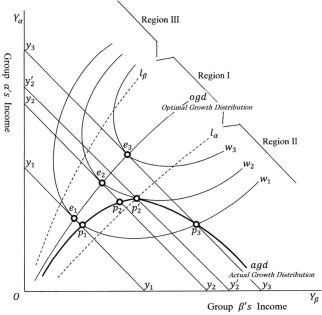
Socially impermissible extreme distribution

We consider the relationship between the increase in income level and social welfare of Group $\alpha$. When the economy grows and total income increases from $y_1$ to $y_2^{{}^{\prime }}$, Group $\alpha$’s income also increases and its income distribution is within the socially permissible borders $l_{\alpha }$ and $l_{\beta }$. In this process, the social welfare increases and approaches the highest attainable level $w_2$. The situation, however, changes remarkably when the total income exceeds $y_2^{{}^{\prime }}$. If the total income increases to $y_3$, the social welfare decreases from $w_2$ to $w_1$. The income share of this point is represented by $p_3$, and this point is located much farther to the right of the permissible border line $l_{\alpha }$. This means that, from the social welfare perspective, the income shares of Group $\alpha$ is extremely low compared to Group $\beta$.

If the total income increases further, the situation becomes more complex. Group $\alpha$ may resent the economic growth in a market economy where they are not rewarded.

Traditional measures for equalisation

Several policies have been presented for the equalisation of income distribution. Two of these policies are discussed here and thereafter the new policy is explained.

The royal road

Progressive taxation of high-income classes and transfer of its revenue to low-income classes is a well-known policy for the equalisation of income distribution (Fig. 3). As the economy grows, the national income $Y$ on the $\mathit{AGD}$ curve is divided between $Y_L$ and $Y_P$. The actual income share is shown as points $P_0,P_1,P_2$, and $P_3$ on the $\mathit{AGD}$ curve.

Fig. 3.

Taxation and transfer

The point $P_3$ is set as the starting point of analysis. The point represents the income distribution between $Y_L$ and $Y_P$ when the national income is $Y_3$. Because this point $P_3$ is considerably to the right of the socially permissible border $L_L$, from the social welfare perspective, the redistribution of income is desirable. At the income level of $Y_3$, the social welfare is maximised at the point $E_3$. To reach this point, it is necessary to tax as much as $P_{3}A$ on the property income and transfer the same amount of tax revenue $A{E}_3$ to labour income. This thoroughgoing measure realizes the maximum social welfare.

The economic value of this progressive taxation and its transfer is inferred as follows: the starting point $P_3$ and attained point $E_3$ are both on the same national income line $Y_3$. The point $P_3$ is on the social welfare indifference curve $W_1$ and its level of social welfare is the same as $E_1$ on the $\mathit{OGD}$ curve. So, although point $P_3$ is on the $Y_3$ line, its economic value from the standpoint of social welfare is equivalent to the income value of $Y_1$. Contrary to the point $P_3$, the attained point $E_3$ is on the social welfare indifference curve $W_3$ and is on the $\mathit{OGD}$ curve. Therefore, the economic value of the progressive taxation and its transfer has the economic value shown by the distance $E_1{E}_3$ or the income difference $Y_3{Y}_1$. This policy is, indeed, extremely efficient to attain maximum social welfare and may be called as ‘the royal road’ to income equalisation.

The royal road policy is ideal for the economy. The rich capitalists (or propertied) class as well as successful entrepreneurs will, however, strongly oppose this policy. One of the most persuasive reasons for opposition is that unlimited progressive taxation will destroy the social order, or extraordinary heavy tax will break their incentive to innovate. If these oppositions are strong, a compromised, downgraded policy is implemented. In this situation, the extent of $P_{3}a$ is taxed and its revenue of $ab(=P_{3}a)$ is transferred. The inequality of income distribution is, then, slightly revised. The economic value of this compromised policy is inferred as the distance $E_1{E}_2$ or the income difference $Y_2{Y}_1$. These down-sized policies are adopted in almost every industrialised economy. But, in many cases, it may not be enough to cope with the ongoing inequality.

Donation (or contribution)

In a market economy, entrepreneurs plan the production and investment scheme to maximise profit, while consumers plan the expenditure and time-allocation scheme to maximise utility. These behaviours come from their self-interest or egoism and are the driving forces of a market economy.8

Altruism (or philanthropy)

At the opposite extreme, there may be altruism or philanthropy. The development of the market economy till now had caused many harmful effects. Nevertheless, it is well known that capitalists, entrepreneurs, and wealthy persons have donated a considerable part of their earnings and properties. The motives for their donation can be classified into three types. First is the pure or genuine altruism motive, such as human welfare and religious sentiments. Second is that of ordinary altruism such as donations or the establishment of foundations with their names. Finally, there is impure or non-genuine altruism such as vanity or pomposity. Currently, due to remarkable innovations, many multi-billionaire entrepreneurs donate their vast wealth to society or establish foundations across the world. These foundations have far-reaching effects. The advancement of art, culture and sciences, support to education and medical activities, and eradication of poverty are well-known examples.

Donations based on the motive of altruism is considered in Fig. 4. The starting point of analysis is set at point $c$ where the labour income is $Y_L^c$ and property income is $Y_P^c$. Here, the existence of property owners’ (i.e. the capitalists’ and entrepreneurs’) utility function $U=U(Y_P,Y_L)$ is supposed, and their income constraint is shown as $Y_P+Y_L=Y_P^c$ ($Y_P^c$: constant). Then, at the point $c$, the property owners’ utility maximisation problem is formulated as:

$$\text{max}U=U\left(Y_P,Y_L\right),\text{subject,to}{Y}_P+Y_L=Y_P^c\left(Y_P^c:\text{constant}\right)$$ 8

Fig. 4.

Altruistic (or Philanthropic) donation

If the property owners have no concern for the income level of labour $Y_L$, or consider the existing level of labour income $Y_L^c$ to be enough, the solution of (8) is a corner solution and attained at point $c$. In this case, the non-altruistic property owners do not donate, and the income distribution is unchanged. Conversely, if the altruistic property owners consider that the existing income distribution is unequal and disadvantageous for labour, they will donate their income to labour. Then, the solution of (8) is shown as:

$$\left(\partial U/\partial Y_L\right)/\left(\partial U/\partial Y_P\right)=1,Y_P+Y_L=Y_P^c$$ 9

In this situation, the altruistic property owners choose, for example, the point $d$ where the property owners’ indifference curve (derived from their utility function $U$) $U_a$ is tangential to the national income line $Y_3{Y}_3$. The altruistic property owners donate their income $cf(=Y_P^c{Y}_P^d)$, and labour receives this. So, the labour income increases to $fd(=Y_L^d{Y}_L^c)$. By virtue of the property owners’ donation, the point of income distribution changes from $c$ to $d$.

Thus, on one hand, the level of social welfare increases from $W_1$ to $W_2$, and, on the other hand, the altruistic property owners’ utility also increases from ${\overline{U}}_a$ to $U_a$. The increase in the utility of property owners is shown in terms of income. The property owners’ indifference curve ${\overline{U}}_a$ is tangential to the income line $Y_a{Y}_a$ at point $g$, which is parallel to $Y_3{Y}_3$. Then, the distance $\mathit{gd}$ represents the increase of property owners’ income and is equivalent to $Y_a{Y}_3$. This income increase may be called as ‘the altruistic donator’s benefit’. The increase in social welfare is also measured in terms of income. As the social welfare increases from $W_1$ to $W_2$, the corresponding equivalent value increases from $E_1$ to $E_2$, meaning that social welfare in terms of income increases to $Y_1{Y}_2$. In Fig. 4, the point $d$ after donation, however, is located to the right of the labour’s socially permissible border line $L_L$. This indicates that although property owners’ donations are valuable, it is insufficient to attain socially optimal income distribution.9

Egoism (or self-protection)

Over time, if the income inequality reaches an extreme, people who become desperately poor or have long been in dire straits will feel strong resentment towards the society, market economy, capitalists, entrepreneurs, and the propertied people. This will lead to social unrest across the country. In such situations, some of the wealthiest people may individually or collectively try to prevent the occurrence of the worst case scenario (such as riots or revolutions) by donating a part of their wealth to the people in need or destitute workers (hereafter, these people are denoted as the destitute).

The behaviour of the wealthiest people is analysed in Fig. 5. The destitute is classified as Group $\alpha$, and the wealthiest is classified as Group $\beta$. In this analysis, only two Groups $\alpha$ and $\beta$ of the society are examined and the rest, whose income is stable, is assumed to be constant and omitted from the analysis.

Fig. 5.

Egoistic (or Self-protective) donation; social unrest effect, utility effect, and income effect

The starting point in the Figure is set at point $h$ (on the $\mathit{agd}$ curve) where the destitute $\alpha$’s income $Y_{\alpha }^h$ is extremely low and that of the wealthiest group $\beta$ is $Y_{\beta }^h$ and is extremely high. First, the existence of the utility function of the wealthiest $U=U(Y_{\alpha },Y_{\beta },I)$ is supposed, where $Y_i(i=\alpha ,\beta )$ is the income of group $i$, and $I$ is the indicator of social unrest brought about by income inequality. This indicator reflects problems between the destitute and wealthiest, demonstrations against income inequality, a riot to achieve economic justice, and so on. Although the indicator $I$ is a function of income inequality, to simplify the analysis, it is assumed as a parameter. In the figure, the indifference curve $U_A$ of the wealthiest group is depicted. At point $H$, which is very close to the neighbourhood of $h$,10 the utility of the wealthiest is maximised.

At point $H$, the indifference curve of the wealthiest $U_A$ is tangential to the income line $y_B{y}_B$. This maximisation problem is formulated as:

$$\text{max}U=U(Y_{\alpha },Y_{\beta },I),\text{subject}\text{to}{Y}_{\alpha }+Y_{\beta }=Y_{\beta }^h(Y_{\beta }^h:\text{constant}),$$ 10

The solution is shown as:

$$\partial U/\partial Y_i=-\lambda ,Y_{\alpha }+Y_{\beta }=Y_{\beta }^h\left(Y_{\beta }^h:\text{constant}\right),$$ 11

where $\lambda$ is a Lagrange multiplier.

The wealthiest $\beta$ at first satisfies the situation shown by point $H$. This point, however, represents the spread of social unrest and the threat felt by the wealthiest $\beta$. If the indicator $I$ which reflects social unrest increases, their utility distinctly decreases (i.e., $\partial U/\partial I<0$), and the shape and location of the utility function $U$ of the wealthiest change and thereby their indifference curves also change. The indifference curve $U_A$ changes to $u_A$. After the increase of the social unrest indicator $I$, the point $H$ is not the optimal point for the wealthiest.11 They seek the point which maximizes their utility and will find that $j$, where the new indifference curve $u_B$ is tangential to the income line $y_B{y}_B$, is the new optimal point. Accordingly, the wealthiest people donate their income by $hk(=Y_{\beta }^h{Y}_{\beta }^j)$, and the destitute receive the same amount as $kj(=Y_{\alpha }^h{Y}_{\alpha }^j)$.

This movement of optimal point from $H$ to $j$ is called ‘the social unrest effect’. It is disintegrated into two parts, i.e. from $H$ to $m$, and from $m$ to $j$. The first movement is that between the points at the same utility level. This movement is called ‘the utility effect’ (of the increase of the social unrest indicator $I$). The second is ‘the income effect’ (of the indicator $I$).

The total and net loss incurred by the wealthiest due to the extreme concentration of wealth which caused social unrest can be considered in the same figure. The total loss is shown as the movement from $m$ to $j$ and $j$ to $n$. This loss is expressed in income terms as $y_A{y}_C$. Because the wealthiest donated their wealth to $\mathit{Hk}$ to mitigate social unrest, their utility level increased from $u_C$ to $u_B$. This leads to the decrease in total loss as $y_B{y}_C$. Then, the net loss caused by the social unrest is shown as $y_A{y}_C-y_B{y}_C$ or $y_A{y}_B$, and this net loss is equal to ‘the income effect’ of the increase in social unrest $I$.

The relationships among ‘the social unrest effect’, ‘the utility effect’, and ‘the income effect’ are shown mathematically as follows:

The social unrest effect is derived from the optimal conditions (11):

$$\left\{\begin{array}{c}{\left(d{Y}_{\alpha }/dI\right)}_{Y_{\beta }^h:const.}\begin{array}{cc}=& \left(U_{\alpha I}-U_{\beta I}\right)/{\mathrm{\Delta }}_I\end{array}\\ {\left(d{Y}_{\beta }/dI\right)}_{Y_{\beta }^h:const.}\begin{array}{cc}=& -\left(U_{\alpha I}-U_{\beta I}\right)/{\mathrm{\Delta }}_I\end{array}\\ \end{array}\right)$$ 12

where $U_{\alpha \beta }={\partial }^{2}U/{\partial Y}_{\beta }\partial Y_{\alpha },U_{\beta \alpha }={\partial }^{2}U/{\partial Y}_{\alpha }\partial Y_{\beta },U_{\alpha \alpha }={\partial }^{2}U/\partial Y_{\alpha }^2,U_{\beta \beta }={\partial }^{2}U/\partial Y_{\beta }^2,U_{\alpha I}={\partial }^{2}U/\partial I\partial Y_{\alpha }$, and $U_{\beta I}={\partial }^{2}U/\partial I\partial Y_{\beta }$. The term ${\mathrm{\Delta }}_I=U_{\alpha \beta }+U_{\beta \alpha }-U_{\alpha \alpha }-U_{\beta \beta }$ is positive from the condition of utility maximisation of the wealthiest.

The utility effect is shown as:

$$\left\{\begin{array}{c}{\left(\frac{\mathrm{\Delta }{Y}_{\alpha }}{{\mathrm{\Delta }}_I}\right)}_{U:const.}=\frac{U_{\alpha I}-U_{\beta I}}{{\mathrm{\Delta }}_I}-\frac{\left(U_I/U_{Y_{\beta }}\right)\left(U_{\alpha \beta }-U_{\beta \beta }\right)}{{\mathrm{\Delta }}_I}\\ {\left(\frac{\mathrm{\Delta }{Y}_{\beta }}{{\mathrm{\Delta }}_I}\right)}_{U:const.}=\frac{-\left(U_{\alpha I}-U_{\beta I}\right)}{{\mathrm{\Delta }}_I}-\frac{\left(U_I/U_{Y_{\beta }}\right)\left(U_{\beta \alpha }-U_{\alpha \alpha }\right)}{{\mathrm{\Delta }}_I}\\ \end{array}\right)$$ 13

The income effect is shown as:

$$\left\{\begin{array}{c}{\left(\frac{\mathrm{\Delta }{Y}_{\alpha }}{\mathrm{\Delta }{Y}_{\beta }^h}\right)}_{I:const.}=\frac{U_{\alpha \beta }-U_{\beta \beta }}{{\mathrm{\Delta }}_I}\\ {\left(\frac{\mathrm{\Delta }{Y}_{\beta }}{\mathrm{\Delta }{Y}_{\beta }^h}\right)}_{I:const.}=\frac{U_{\beta \alpha }-U_{\alpha \alpha }}{{\mathrm{\Delta }}_I}\\ \end{array}\right)$$ 14

Therefore, by considering the Eqs. (12) ~ (14), the social unrest effect or the total effect is rewritten as:

$$\left\{\begin{array}{c}{\left(d{Y}_{\alpha }/dI\right)}_{Y_{\beta }^h:const.}={\left(d{Y}_{\alpha }/dI\right)}_{U:const.}+\left(U_I/U_{Y_{\beta }}\right){\left(d{Y}_{\alpha }/d{Y}_{\beta }^h\right)}_{I:const.}\\ {\left(d{Y}_{\beta }/dI\right)}_{Y_{\beta }^h:const.}={\left(d{Y}_{\beta }/dI\right)}_{U:const.}+\left(U_I/U_{Y_{\beta }}\right){\left(d{Y}_{\beta }/d{Y}_{\beta }^h\right)}_{I:const.}\\ \end{array}\right)$$ 15

where $U_I=\partial U/\partial I<0$ and $U_{Y_{\beta }}=\partial U/\partial Y_{\beta }$.

As to the signs of Eqs. (12–15), no confirmed inference can be obtained without additional assumptions. The concrete determination of signs is, however, obtained from the situation depicted in Fig. 5. In this specific situation, the following conclusions are derived:

As to the utility effect,

$${\left({\mathit{dY}}_{\alpha },/,d,I\right)}_{U:const.}>0,{\left({\mathit{dY}}_{\beta },/,d,I\right)}_{U:const.}<0$$ 13’

As to the income effect,

$${\left(d,Y_{\alpha },/,d,Y_{\beta }^h\right)}_{I:const.}<0,{\left(d,Y_{\beta },/,d,Y_{\beta }^h\right)}_{I:const.}<0$$ 14’

As to the social unrest effect or total effect,

$${\left(d,Y_{\alpha },/,d,I\right)}_{Y_{\beta }^h:const.}>0,{\left(d,Y_{\beta },/,d,I\right)}_{Y_{\beta }^h:const.}<0$$ 15’

The change in social welfare is next considered briefly in Fig. 6. The optimal point moved from $H$ to $j$ due to the egoistic donation of the wealthiest. According to this movement, the level of social welfare increases from w ₁ to w ₂, and the corresponding equivalent value increases from $e_1$ to $e_2$. This implies that even if the motive of donation is egoistic, the donation contributes to the increase in the level of social welfare. However, the point $j$ after the donation is located to the right of the socially permissible line of the destitute $l_{\alpha }$. This indicates that the egoistic donation of the wealthiest group is insufficient to resolve the difficult situation.

Fig. 6.

Egoistic (or Self-Protective) donation and its effect on social welfare

Erasure of government bonds

Although ‘helicopter money’ and ‘MMT’ policies have a wide range of purposes, they are effective in managing income inequality. It is reasonable to implement these policy measures if the price level is stable.

Japan as an example: the amendment of law and erasure

After evaluating the above policies, this study proposes a new policy to mitigate or overcome the income distribution inequality. The policy is that, by amendment of law, the government erases the government bonds (owned by the central bank) for income equalisation.

This study considers Japan as an example. At the end of September 2021, the amount of outstanding government bonds is approximately 9.5 trillion dollars, which is a little less than twice as much as Japan’s GDP.12 The ratio, government bonds outstanding/GDP, is the highest (or worst) in the industrialised countries, leading to fears of bankruptcy of the Japanese government. BOJ owns approximately 4.6 trillion dollars. By subtracting 4.6 trillion dollars from 9.5 trillion dollars, 4.9 trillion dollars remain. If this amount is divided by the GDP, the quotient is about 1.0. So, the ratio of the debt burden decreases drastically,13 which is the key issue.

If 4.6 trillion dollars of government bonds owned by BOJ remain intact and 9.5 trillion dollars of total government bonds remain, problems will occur because of the following reasons: first, because the government bonds outstanding is 1.9 times as large as Japan’s GDP, the exogenous shocks such as war, massive earthquakes, endogenous great depressions, and pandemics can cause unexpected scenarios. Second, if massive amounts of government bonds remain intact, consumers will anticipate a future tax increase and feel uneasy about their social security, medical care, education, and so on, and refrain from consumption as much as possible. Moreover, entrepreneurs will expect an increase in corporate tax and after surveying the attitude of consumers, will hesitate to invest.

When massive and enduring government bonds (or debts) exist, the economy has the tendency towards nearly zero rate of growth or stagnation. Therefore, people who slid down from the middle class to the low-income class and low-income group people are forced to endure this situation.

Therefore, the government bonds which the central bank possesses should be erased. This measure will minimise the fear of tax increase, and consumers’ and entrepreneurs’ psychological pressure will be significantly reduced. From the macroeconomic perspective, both the consumption function and investment function will shift favourably.

Regarding the side effects of the erasure policy, heavy confusion regarding the bonds market or the economy may be anticipated. However, the side effects are limited. As the amount of government bonds decreases drastically, and the government bonds held by private sectors and foreign countries are not erased and guaranteed firmly, its scarcity value will increase. The possibility of the default of Japan’s government bonds will vanish. This will increase the demand for Japan’s government bonds which in turn will increase its price leading to a decrease in the interest rate.

New issue of government bonds for equalisation

After the erasure of the existing government bonds, new government bonds need to be issued to equalise income distribution. The generated revenue is spent on low-income people. This increases their income level and improves their health condition, provides opportunity for higher education, human capital formation to increase their productivity, and so on. Therefore, their future income will continuously increase. These strong measures will improve low-income situations and lead the whole economy towards steady growth.

The summated issue depends on the sum needed to equalise income distribution, but it should not exceed the erased sum. This ensures that debts do not accumulate.

In Japan’s case, the amount of outstanding government bonds is now approximately 9.5 trillion dollars and, of these, BOJ owns about 4.6 trillion dollars. After the amendment of the law, the government of Japan erases these 4.5 trillion dollars of government bonds held by BOJ. The remaining government bonds (5.0 trillion dollars) are still owned by domestic and foreign investors.14 The government must firmly guarantee the obligation. As the possibility of default completely disappears by the erasure of government bonds (held by BOJ), the scarcity value of the 5 trillion dollars of government bonds will increase, thereby increasing the demand for Japanese government bonds. Specifically, there will be an excess demand for Japanese government bonds.

To realize the optimal income equalisation, I consider how much the government should expend for the low-income people. In this model, to simplify the analysis, the labour income is considered to be that of low-income people.

Given the existing property income level, the total socially optimal sum $R$ required for income distribution is defined as:

$$\text{R}\text{=}\text{the}\text{labour's}\text{socially}\text{optimal}\text{income}\text{level}\text{- the}\text{labour's}\text{existing}\text{income}\text{level}$$ 16

where the labour’s socially optimal income level satisfies the optimal conditions (4).

I consider the above using an abstract example and then a numerical example which may also have an empirical reality.

The initially erased sum is denoted as $A$. The total optimal sum required for income equalisation is assumed to be $R$ trillion dollars.

To avoid rapid changes which will be caused by the lump-sum expenditure of $R$, the process of further erasure and expenditure should be divided into a geometric series. These divisions will be useful to smoothen the change and constrain the occurrence of inflation. If, during these processes, inflation occurs, the erasure and expenditure policy should be suspended and resumed after the resolution of inflation. The upper limit of the inflation is about 2%.

The first step is to newly issue some ratio of the erased sum. This ratio is called ‘newly issued rate’, denoted by $\varphi$, i.e.

$$\text{newly}\text{issued}\text{rate}\varphi =\frac{\text{newly}\text{issued}\text{government}\text{bonds}}{\text{initially}\text{erased}\text{government}\text{bonds}\text{A}},(1>\varphi >0)$$ 17

The newly issued government bonds are denoted as $\varphi A$. This sum $\varphi A$ is expended for the low-income group, which involves social security including reinforcement of the pension system, medical care, education for human capital formation to enhance their future earning capacities, and assistance for undeveloped countries (the income redistribution for foreign low-income group). These will increase the welfare of the low-income group and consequently increase their economic productivity. Then, because the government bonds have increased to $\varphi A$, the government erases ${\varphi }^{2}A$ of the government bonds. The residual non-erased portion $\left(1,-,\varphi \right)\varphi A$ is still held by domestic and foreign investors and firmly guaranteed by the government. The above process is shown as follows:

The second step is to issue new government bonds by as much as ${\varphi }^{3}A$ and expend the same amount for the low-income group. Then, of these increased bonds, the government erases ${\varphi }^{4}A$ and the residual non-erased portion $\left(1,-,\varphi \right){\varphi }^{3}A$ held by domestic and foreign investors is firmly guaranteed by the government. This process is shown as follows:

The third step is similarly shown as:

To summarize these steps $\left(\text{PI}\right),\left(\text{PII}\right),\left(\text{PIII}\right),\cdots$, the total optimal expenditure $R$ for the low-income group is equal to:

$$R=\varphi A+{\varphi }^{3}A+{\varphi }^{5}A+\cdots =A\varphi /(1-{\varphi }^2)$$ 18

From this, the value of $\varphi$ is calculated as:

$$\varphi =\left(-,A,+,\sqrt{A^2+4R^2}\right)/2R$$ 19

When the government’s optimal expenditure $R$ for the low-income group is implemented gradually, the multiplier effects work at each step. If the scale of its effects is $m$, the total created income $V$ is shown as:

$$V=m\varphi A+m{\varphi }^{3}A+m{\varphi }^{5}A+\cdots =mA\varphi /(1-{\varphi }^2)$$ 20

The total residual non-erased sum $S$ which is held by domestic and foreign investors is calculated as:

$$\mathrm{S}=\left(1,-,\varphi \right)\varphi A+\left(1,-,\varphi \right){\varphi }^{3}A+\left(1,-,\varphi \right){\varphi }^{5}A+\cdots =A\varphi /(1+\varphi )$$ 21

By such increases in created income, tax revenues also increase. If the average and marginal tax rate is denoted as $t$, the total increases of tax revenue $T$ is:

$$T=tm\varphi A+tm{\varphi }^{3}A+tm{\varphi }^{5}A+\cdots =tmA\varphi /(1-{\varphi }^2)$$ 22

If this tax revenue $T$ is used to redeem the government bonds, the net increase of government bonds $N(=\mathrm{S}-T)$ is:

$$N=S-T=A\varphi \left(1,-,\varphi ,-,t,m\right)/(1-{\varphi }^2)$$ 23

If the government bonds that were outstanding before the erasure policy is denoted as $Z$, the total sum of government bonds held by domestic and foreign (including government) investors $\mathrm{\Sigma }$ is:

$$\mathrm{\Sigma }=Z-A+N=Z-A+A\varphi \left(1,-,\varphi ,-,t,m\right)/(1-{\varphi }^2)$$ 24

The above expressions (18–24) are elucidated using numerical examples. First, the expressions (18–20) are explained diagrammatically.

Because government’s first erased sum $A$ is 4.50 trillion dollars, if the total optimal sum $R$ required for income redistribution is, for example, 3 trillion dollars, the government’s new issue rate $\varphi$ can be obtained by calculating the expression (18), i.e.

$$3.00=4.50\varphi /(1-{\varphi }^2)$$ 25

From this, the value of $\varphi$ is determined as 0.50. This implies that if the government has a heavy burden of outstanding government bonds of 9.50 trillion dollars (out of which BOJ holds 4.60 trillion dollars) and needs 3 trillion dollars to expend for optimal income redistribution, the government should erase 4.50 trillion dollars of government bonds held by BOJ and, in the first period, newly issue the $0.50\times 4.50\mathrm{trilion}\mathrm{dollars}=2.25$ trillion dollars of government bonds for income redistribution and, in the second period, newly issue the ${0.50}^3\times 4.50=0.56$ trillion dollars of government bonds for income redistribution and, in the third period, ${0.50}^5\times 4.50=0.14$ trillion dollars of government bonds, $\cdots$. Then, from Eq. (18), the following relationship is obtained:

$$\begin{array}{cc}3.00& \fallingdotseq \\ \text{Required}\text{sum}& \fallingdotseq \end{array}\begin{array}{cc}2.25& +\\ \text{first}\text{period}& +\end{array}\begin{array}{cc}0.56& +\\ \text{second}\text{period}& +\end{array}\begin{array}{c}0.14\\ \text{third}\text{period}\end{array}\begin{array}{c}+\\ +\end{array}\begin{array}{c}\dots \\ \dots \end{array}$$ 18’

Here, to implement the income equalisation, expenditure should be made over the years to make the transfer payment and construction of various systems (such as social security, medical care, education, foreign assistances, etc.) smooth. Beside these, gradual steps of expenditure are indispensable to avoid inflation.

If the multiplier effect over all period is 2.00, the total created income $V(=2.00R)$ is shown as:

$$V=2.25\times 2.00+0.56\times 2.00+0.14\times 2.00+0.04\times 2.00+\cdots \fallingdotseq 6.00\left(\text{trillion}\text{dollars}\right)$$

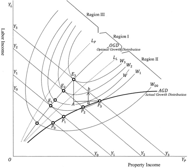
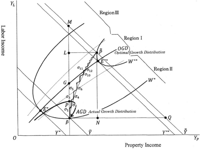
The effect of optimal redistribution money $R$ on income creation $V$ and social welfare $W$ is explained in Fig. 7. The starting point is $P_4$ where the erasure of government bonds held by central bank has been completed. The total optimal sum $R$ required for income equalisation is shown as the distance $P_{4}g$ where the point $g$ is on the $\mathit{OGD}$ curve and therefore this point $g$ satisfies the social optimal conditions (4).

Fig. 7.

The effect of expenditure on income equalization

At point $P_4$, the property income is shown as $\mathit{Oe}$. From the social welfare point of view, the optimal level of labour income is $\mathit{eg}$. The existing level of labour income is $e{P}_4$. So, the total optimal sum $R$ required for income equalisation is:

$$R=eg-e{P}_4=P_{4}g$$ 26

It is assumed that $R$ is equal to 3.00 trillion dollars, or $P_{4}g=3.00\text{trillion dollars}$. To finance this sum and to not accumulate too much debt, I proposed to erase nearly all of the 4.50 trillion government bonds held by BOJ and to issue new government bonds which amounts to half of the total erased sum. Through this, the government obtains 2.25 trillion dollars. The process starts and continues as follows: First, 2.25 trillion dollars are divided, for example, by 5 and, each 0.45(= 2.25/5) trillion dollars are expended over five years.

The first year’s expenditure is shown as $P_4{\rho }_1$ and taking into its multiplier effect 2.00, the expenditure creates additional income shown as ${\rho }_1{\rho }_2$. The next year’s expenditure is shown as ${\rho }_2{\rho }_3$ and by the multiplier effect, this expenditure creates the additional income ${\rho }_3{\rho }_4$. This process continues to the point ${\rho }_{10}$, where the redistributed money is 2.25 trillion dollars and the total additional income is 4.50(= 2.25 × 2.00) trillion dollars.

Second, 0.56 trillion dollars are divided by 5 and each 0.11(= 0.56/5) trillion dollars are expended over five years. This year’s expenditure is shown as ${\rho }_{10}{\rho }_{11}$, and it creates additional income ${\rho }_{11}{\rho }_{12,\cdots }$. These processes go on till point $P_5$. The sum of redistributed money $R$ is 3.00 trillion dollars and the total created income $V$ is 6.00 trillion dollars. The total increased income $V$ is shown as $Y_4{Y}_5$ (or $P_{4}m$, or $P_{4}q$) and of this income $V$, the increased labour income is shown as $P_{4}l(=nq)$ and increased property income is $lm(=P_{4}n)$.

It is shown that by the introduction of optimal redistribution of money $R$, the level of social welfare increases from $W_0$ to $W_5$, and the economic value increases from $E_0$ to $E_5$. The result of this policy expressed in terms of income is $Y_4{Y}_5$.

Next, the expressions (21–24) are explained. The sum of government bonds newly issued (but not erased) and purchased by domestic and foreign investors $S$ (trillion dollars), i.e. the total residual non-erased sum is calculated as:

$$S=1.13+0.28+0.07+0.02+\cdots \fallingdotseq 1.50(\mathrm{trillion}\mathrm{dollars})$$

The total increase in tax revenue brought about by the created income is calculated. If the average and marginal income tax rate is 0.20, the total increase in tax revenue $T$ is shown as:

$$T=0.20V=2.25\times 2.00\times 0.20+0.56\times 2.00\times 0.20+0.14\times 2.00\times 0.20+0.04\times 2.00\times 0.20+\cdots \fallingdotseq 1.20\left(\text{trillion}\text{dollars}\right)$$

Then, if this tax revenue is used to redeem the government bonds, the net increase in government bonds can be calculated. The sum $N(=S-T)$ is shown as:

$$N\left(=,S,-,T\right)\fallingdotseq 1.50-1.20=0.30\left(\text{trillion}\text{dollars}\right))$$

Hence, the total sum of government bonds held by domestic and foreign investors $\mathrm{\Sigma }$ (trillion dollars) is shown as:

$$\mathrm{\Sigma }=5.00+0.30=5.30\left(\text{trillion}\text{dollars}\right)$$

The above numerical example is summarized as follows: when the total optimal expenditure $R$ is needed by 3.00 trillion dollars, the erasure rule demands that newly issued rate $\varphi$ should be 0.50. If the multiplier effects $m$ on redistribution expenditure $R$ is 2.00, the total created income $V$ becomes $2R$ or 6.00 trillion dollars. The total residual non-erased sum $S$ is 1.50 trillion dollars. If the average and marginal tax rate $t$ is 0.20, the total increase of tax revenue $T$ is $0.20V$ or 1.20 trillion dollars. The net increase in government bonds $N(=S-T)$ is therefore $1.50-1.20=0.30$ trillion dollars. As a result, the total sum of government bonds $\mathrm{\Sigma }\left(=,5.00,+,0.30\right)$ is equal to 5.30 trillion dollars.

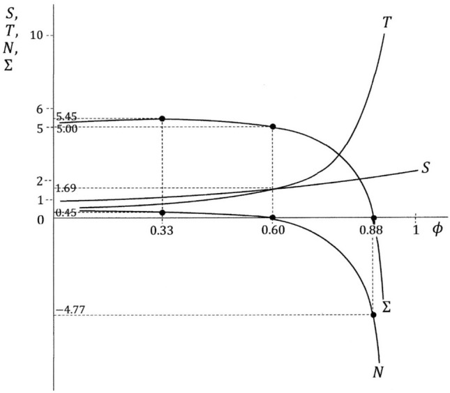
Other values of total optimal expenditure for redistribution $R$ are also examined. These are shown in Table 1. The table shows the relationship between $R$ and $\varphi ,V,S,T,N$, and $\mathrm{\Sigma }$ (when the value of multiplier effect $m$ is 2.00, and tax rate is 0.20).

Table 1.

The Relationship between $R$ and $\varphi ,V,S,T,N$, and $\mathrm{\Sigma }$

Total optimal sum for redistribution	$R$	1.00	1.67	2.00	3.00	4.22	5.00	…	10.00	…	17.21	…	21.32	…	25.00
Newly issue rate	$\varphi$	0.21	0.33	0.38	0.50	0.60	0.65		0.80		0.88		0.90		0.91
Total created income	$V=2R$	2.00	3.34	4.00	6.00	8.44	10.00		20.00		34.42		42.64		50.00
Total residual non erased sum	$S$	0.78	1.12	1.24	1.50	1.69	1.77		2.00		2.11		2.13		2.14
Total increase of tax revenue	$T=0.4R$	0.40	0.67	0.80	1.20	1.69	2.00		4.00		6.88		8.53		10.00
Net increase of government bonds	$N=S-T$	0.38	0.45	0.44	0.30	0.00	− 0.23		− 2.00		− 4.77		− 6.40		− 7.86
Total sum of Government bonds outstanding	$\mathrm{\Sigma }=$ $5.00+N$	5.38	5.45	5.44	5.30	5.00	4.77		3.00		0.23		− 1.40		− 2.86

$R=\frac{\varphi A}{1-{\varphi }^2},\varphi =\mathrm{newly}\mathrm{issued}\mathrm{government}\mathrm{bonds}/\mathrm{erased}\mathrm{government}\mathrm{bonds},$

$A=4.50\mathrm{trillion}\mathrm{dollars},Z=9.50\mathrm{trillion}\mathrm{dollars},V=mR,S=\frac{\varphi A}{1+\varphi },$

$N=\frac{\varphi A\left(1,-,\varphi ,-,m,t\right)}{1-{\varphi }^2},\mathrm{\Sigma }=Z-A+\frac{\varphi A\left(1,-,\varphi ,-,m,t\right)}{1-{\varphi }^2},m=2.00,t=0.20$

From Table 1, two relationships are established and considered.

One is the relationship between $R$ and $\varphi$, depicted as the curve $R$ in Fig. 8. The slope of this curve $R$ is positive and increasing, i.e. $\partial R/\partial \varphi >0$ and ${\partial }^{2}R/\partial {\varphi }^2>0$.15 The curve $R$ shows that, given the value of the initially erased sum $A$, when the total optimal sum $R$ is determined, the newly issue rate $\varphi$ is correspondingly calculated. This figure is intended to be read from the vertical axis to the horizontal axis, or from $R$ to $\varphi$. Therefore, if the total optimal sum $R$ required for income equalisation is 1.67 trillion dollars, the newly issued rate $\varphi$ is determined as 0.33, and if $R$ is 4.22, $\varphi$ is 0.60.

Fig. 8.

The relationship between the total optimal sum $R$ and newly issued rate $\varphi$

Another relationship is between $\varphi$ and $S,T,N(=S-T)$ and $\mathrm{\Sigma }(=5.00+N)$, depicted in Fig. 9. The relationship between the total residual non-erased sum $S$ and $\varphi$ is shown as $S$ curve. The slope of this curve $S$ is positive and decreasing.16 The relationship between the total increase in tax revenue $T$ and $\varphi$ is shown as the $T$ curve, and the slope of this $T$ curve is positive and increasing.17 The net increase in government bonds $N$ is equal to $\mathrm{S}-T$. The curvature of the curve $N$ is convex and sloping upwards18 and reaches a maximum point when $\varphi$ is equal to 0.33.19 By connecting these two figures, the relationship between the total optimal sum for redistribution $R$ and net increase in government bonds $N$, and the total sum of government bonds outstanding $\mathrm{\Sigma }(=5.00+\mathrm{N})$ is shown. This study explains three characteristic points:

1. When the optimal sum for redistribution $R$ is 1.67 trillion dollars, the newly issued rate $\varphi$ is 0.33. At this rate, as explained above, the net increase in government bonds $N$ reaches the peak, and the total sum of government bonds outstanding $\mathrm{\Sigma }$ reaches the peak. In the interval of $0<\varphi <0.33$, $N$ and $\mathrm{\Sigma }$ increase, and in the interval of $0.33<\varphi <1$, $N$ and $\mathrm{\Sigma }$ decrease.

2. When $R$ is 4.22 trillion dollars, $\varphi$ is 0.60. At this rate, the total residual non-erased sum $S$ is equal to the total increase in tax revenue, and therefore $N$ becomes zero. This means that total sum of government bonds outstanding $\mathrm{\Sigma }$ is 5 trillion dollars which is equivalent to the sum before the new issue of government bonds.

3. When $R$ is 17.21 trillion dollars, $\varphi =0.88$. At this rate, $S$ is 2.11 trillion dollars and $T$ is 6.88 trillion dollars. Thus, the net increase in government bonds $N$ becomes -4.77 trillion dollars, and the total sum of government bonds outstanding $\mathrm{\Sigma }$ becomes 0.23 trillion dollars, or nearly zero. This means that the outstanding government bonds almost disappear.20

Fig. 9.

The relationship between $\varphi$ and total created income $V$, total residual non-erased sum $S$, total increase in tax revenue $T$, net increase in government bonds $N(=S-T)$, and total sum of outstanding government bonds $\mathrm{\Sigma }$

It must be noted that because the optimal value of $R$ is determined from the (constrained) social welfare maximisation conditions (4), the level of total sum of government bonds outstanding $\mathrm{\Sigma }$ is not the object of some sort of maximisation, but the result of the determination of $R$. In other words, social welfare maximisation conditions determine the values of $R,\varphi ,V,S,T,N$, and $\mathrm{\Sigma }$.

It is natural that the relatively small sum of $R$ is easily carried out. But, using the method of erasing government bonds, the relatively large sum of $R$ is carried out without accumulating government bonds or with decreasing government bonds. The government can revise income inequality if it wishes to do so.

The pandemic and income equalisation

History reveals that humankind has suffered from many disasters. One of the most serious disasters is the COVID-19 pandemic. The prevalence of the plague, smallpox, cholera, new influenza, and new coronavirus are the representative epidemics. From the income inequality perspective, high-income groups seem to have a relatively advantageous position in avoiding infectious diseases. This is because the high-income groups live in a favourable environment (good sanitary conditions, housing, access to medical facilities, education regarding hygiene, etc.). Conversely, low-income groups lack these facilities which leaves them vulnerable to serious infectious diseases. Thus, income distribution inequality causes the unequal susceptibility to epidemics and diseases. If the pandemic spreads worldwide, its victims will mostly be a part of the low-income group than the high-income group.

During the pandemic, governments take drastic measures such as closing the borders and restricting the movement of people and commodities. If the situation persists, the total demand and supply of the economy substantially decreases which has a negative impact on economic activities. The high-income group also suffers tremendous losses, but, owing to their accumulated wealth, many of them can deal with it. In contrast, if low-income groups lose their jobs, they get into a predicament. Thus, the pandemic affects the low-income group more than the high-income group.

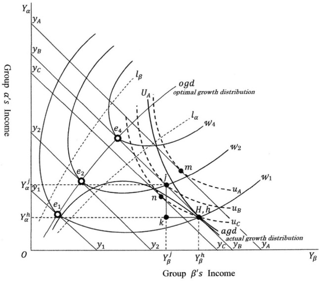
Governments need to take prompt and adequate measures to tackle the pandemic. One suitable measure is the income equalisation or payment of adequate benefits to low-income groups. Figure 10 explains this. The point $P$ on the $\mathit{AGD}$ curve shows the income level and its distribution before the outbreak of pandemic. As the pandemic becomes severe, the economic situation worsens and the point on the $\mathit{AGD}$ curve moves from $P$ to $\tilde{P}$. This movement shows the high disadvantage for the low-income group. Both the absolute income level and relative income share of low-income group decreases. To resolve this grave situation, the government needs to revise the inequality. The following numerical example explains this. At the point $P$ which represents the situation before pandemic, the total optimal sum required for income equalisation $R$ is shown as the distance $\mathit{PG}$ and its amount is assumed to be 3.00 trillion dollars. The economic situation moves down to $\tilde{P}$ due to the outbreak and spread of the pandemic. This indicates that, to revise the inequality completely, $R$ must be the distance $\tilde{P}G$ and this amount is assumed to be 5.00 trillion dollars.

Fig. 10.

Pandemic and the effect of expenditure on income equalization

To revise this severe inequality, 5.00 trillion dollars should be expended for low-income groups. The process and results are shown in Table. If $R$ is equal to 5.00 (trillion dollars), the newly issued rate $\varphi$ is set at 0.65 (percent). If the multiplier effect of $R$ is 2.00, the total created income $V$ is 10.00 (million dollars). The total residual non-erased sum $S$ is 1.77 (trillion dollars). If the average and marginal tax rate $t$ is 0.20, the total increase in tax revenue $T$ is 2.00 (trillion dollars). Then, the net increase in government bonds decreases. As a result, the total sum of government bonds outstanding $\mathrm{\Sigma }$ is 4.77 (trillion dollars), which is below the initial level of 5.00.

Through this process, the economy grows from $\tilde{Y}$ to $\widetilde{\stackrel{~}{Y}}$, and the increment of national income $\mathrm{\Delta }\mathrm{Y}$ is equal to $2R(=10\mathrm{trillion}\mathrm{dollars})$. The low-income group who was facing challenges are now better off. Their income level increases to $\tilde{P}L$. The level of social welfare has increased from $W^{\ast }$ to $W^{\ast \ast }$, and its economic value is expressed as the increase in income level from $Y^{\ast }$ to $Y^{\ast \ast }$.

This policy is summarized as follows: the 5.00 trillion dollars of income equalisation expenditure creates 10.00 trillion dollars of national income, and by the policy of erasure of government bonds and multiplier effect, the net increase in government bonds is approximately zero. The income level of the low-income group and level of social welfare improves significantly.

Apprehension regarding inflation

This section examines inflation. This study considers that, compared to the previous century, the probability of inflation is not so high currently. Two factors may be stated:

First, as is widely supported, after the end of the Cold War, countries, such as China, India, Russia, and many others entered the world market economy. These countries provided high-quality goods with reasonable prices. The industrialised countries imported these goods which reduced the domestic prices of the goods. These tendencies are pervasive and will persist unless irregular exogenous shocks hit the economy.

Second, especially after the public access to the Internet, the world economy is now in a severe competition to innovate in the IoT field. Conventional goods and services are substituted by those made by high-technology companies. Such goods are not always cheap. However, as the efficiency of IoT industries is remarkably high, the hedonic prices of these goods are showing a downward trend due to technological progress induced by tough competition.

Third, the price of energy will not surge for a long time. Alternative energy is now being developed. An example is shale oil and shale gas. Shale oil and gas reserves are abundant.21 In addition to this, the worldwide prevalence of the development and utilization of renewable energy will resist any energy price increase.

The above-mentioned reasons will suppress the possibility of future inflation. However, the possibility of the occurrence of inflation cannot be dismissed.22 If the expenditure for income equalisation $R$ affects the inflation rate $i$, this relationship is shown as:

$$i=i(R,\overline{F})$$ 27

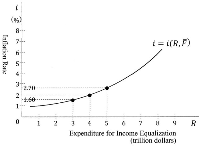
where $\overline{F}$ is the other factors which affect the inflation rate $i$, and to simplify the analysis, assumed to be constant. Regarding the shape of the function $i$, the following relationships are assumed: $di/dR\geqq 0$ and $d^{2}i/d{R}^2\geqq 0$. This function $i$ is shown in Fig. 11. This hypothetical curve $i$ represents that when the value of $R$ is 3.00 trillion dollars, the inflation rate $i$ is 1.60%, when $R$ is 4.00 trillion dollars, $i$ is 2.00%, and when $R$ is 5.00 trillion dollars, $i$ becomes 2.70%.

Fig. 11.

The relationship between the total optimal sum $R$ and inflation rate $i$

Thus, when the society or government opposes the inflation rate which exceeds 2%, the scale of the expenditure for income equalisation $R$ is constrained by this inflation rate. In this situation, if, for example, 3.00 trillion dollars of $R$ is planned, this may be permitted from the standpoint of controlling inflation. If, however, 5.00 trillion of $R$ is planned, this may not be permitted.23 As inflation occurs also due to the other factors, to avoid an undesirable rate of inflation, these factors must be taken into account.

If by any chance,24 an undesirably high inflation rate occurs, the countermeasure is to absorb the money in the market. The government should issue government bonds. If the amount of this issue is too much, the price of government bonds will fall and the interest rate will rise. If this happens in a short time, many of the domestic and foreign investors will suffer huge losses. The government does not suffer any loss because, by erasure, government has little government bonds outstanding. It must, however, be stressed that inflation negatively affects the low-income group, but, by this policy, as the low-income group upgrades to the middle income group, from the income distribution perspective, the inflation does not exert too much negative impact. As long as the inflation rate is low, the majority does not suffer. If a high inflation rate occurs, the policy of erasure and expenditure for the low-income group should be discontinued for some time and resumed after the resolution of inflation.

Multiplier analysis

This section considers the above policy measure, i.e. income equalizing expenditure $R$, and then compares the effectiveness between it and public investment for countercyclical purpose $G$.

First, the consumption function $C$ is expressed as:

$$C=C\left(Y,-,T,+,R,,,Y^f,(R,G)\right)$$ 28

where $T$ is the tax and is assumed to be proportional to national income $Y$, i.e. denoting $t$ as an average and marginal tax rate, $T=tY$. $R$ is the government expenditure for income equalisation.25 Then, $Y-T+R$ represents the disposable income in a broad sense. $Y^f$ is the future income which is assumed to depend on government expenditure for income equalisation $R$ and public investment for countercyclical measures $G$, i.e. $Y^f=Y^f(R,G)$. The study assumes the following relationships: $1>\partial C/\partial (Y-T+R)>0,1>\partial C/{\partial Y}^f>0,\partial Y^f/\partial R>0$, and $\partial Y^f/\partial G<0$.26

Second, the investment function $I$ is expressed as:

$$I=I\left(r,\left(R,,,G\right),,E(R,a,\left(G\right),,,b,(G)\right)$$ 29

where $r$ is the market interest rate which is assumed to be influenced by the government expenditure for income equalisation $R$ and public investment $G$,27 i.e. $r=r(R,G)$. When the parameters $R$ and $G$ increase, $r$ may increase a little. Thus, the following relationships are assumed: $\partial r/\partial R\geqq 0,\partial r/\partial G\geqq 0$, and as to the relationship between $r$ and $I$, it is assumed to be negative, i.e. $\partial I/\partial r<0$. $E$ is a factor which is related to the efficiency of investment $I$ and depends on $R$ and $G$. I call $E$ ‘an efficient factor in investment’. When $R$ increases, the income of low-income people also increases. Through this, people can be better off and have the opportunity to learn more, and are able to improve their health conditions. In this situation, the efficiency of investment $I$ will increase. Therefore, the following relationships are assumed: $\partial I/\partial E>0$ and $\partial E/\partial R>0$. As to the effects of public investment for countercyclical purpose $G$ on investment$I$, two effects are supposed. One is the improvement in infrastructure and through this, investment efficiency will increase. This effect is called the ‘infrastructure effect’ and denoted as $a$ and calculated by: $a=a\left(G\right),da/dG>0,dE/da>0$, and $dI/dE>0$. Another is investing in pork-barrel public projects, which is often done so that politicians can secure votes, which have negative effects on the investment efficiency $I$. This effect is called the ‘futility effect’ and denoted as $b$ and calculated by: $b=b\left(G\right),db/dG>0,dE/db<0$, and $dI/dE>0$.

The equation for the determination of national income is:

$$Y=C\left(Y,-,T,+,R,,,Y^f,(R,G)\right)+I\left(r,\left(R,,,G\right),,E(R,a,\left(G\right),,,b,(G)\right)+R+G$$ 30

The effect of distribution equalizing expenditure $R$ on the national income $Y$ is calculated as follows:

$$\frac{\mathit{dY}}{\mathit{dR}}=\left[1,+,\frac{\partial C}{\partial (Y-T+R)},+,\frac{\partial C}{\partial Y^f},\frac{\partial Y^f}{\partial R},+,\frac{\partial I}{\partial r},\frac{\partial r}{\partial R},+,\frac{\partial I}{\partial E},\frac{\partial E}{\partial R}\right]/\left[1,-,\frac{\partial C}{\partial \left(Y,-,T,+,R\right)},(1-t)\right]$$ 31

From the assumptions above, the denominator of (31) is positive. Among the terms of the numerator, the term $\left(\partial ,I,/,\partial ,r\right)\left(\partial ,r,/,\partial ,R\right)$ is nearly zero or zero.28 However, a negative value of this term will not overwhelm the total positive values of the other terms. So, the numerator will be positive. Then, as to the sign of (31), the following relationship may hold:

$$dY/dR>0$$ 32

The effects of the government’s distribution equalizing expenditure $R$ on the labour income $Y_L$ and property income $Y_P$ can be analysed. In Fig. 7, the tangent line of the actual growth distribution curve $\mathit{AGD}$ at point $P_4$ is expressed as

$$Y_L=\alpha Y_P+\beta \left(\alpha =\alpha \left(R\right),\beta :\text{constant}\right)$$ 33

where it is assumed that $\alpha$ depends on the parameter $R$, i.e. $\alpha =\alpha (R)$ and $\alpha (R)$ is positive and $d\alpha /dR$ is also positive.29 This tangential line means that the change in the parameter $R$ affects the relationship between $Y_L$ and $Y_P$; i.e. if $R$ changes, the following relationship holds: $d{Y}_L={\alpha }^{{}^{\prime }}{Y}_{P}dR+\alpha {\mathit{dY}}_P$, where ${\alpha }^{{}^{\prime }}=d\alpha /dR$.

As $Y=Y_L+Y_P$, the Eq. (30) is revised as:

$$Y_L+Y_P=C\left(\left(1-t_L\right)Y_L+\left(1-t_P\right)Y_P+R,Y^f\left(R,G\right)\right)+I\left(r\left(R,G\right),E(R,a\left(G\right),b\left(G\right)\right)+R+G$$ 34

where $t_L$ and $t_P$ are the income tax rate on $Y_L$ and $Y_P$, respectively, and $t_L<t_P$. From (34), the following relationships are obtained:

$$\frac{d{Y}_L}{\mathit{dR}}=\frac{{\alpha }^{\prime }{Y}_P\left\{1-C^{\prime }·\left(1-t_P\right)\right\}+\alpha \left(C^{\prime }+1\right)+\alpha \left(\frac{\partial C}{\partial Y^f}\frac{\partial Y^f}{\partial R}+\frac{\partial I}{\partial r}\frac{\partial r}{\partial R}+\frac{\partial I}{\partial E}\frac{\partial E}{\partial R}\right)}{1-C^{\prime }·\left(1-t_P\right)+\alpha \left\{1-C^{\prime }·\left(1-t_L\right)\right\}}$$ 35

$$\frac{d{Y}_P}{\mathit{dR}}=\frac{-{\alpha }^{{}^{\prime }}{Y}_P\left\{1-C^{{}^{\prime }}·\left(1-t_L\right)\right\}+C^{{}^{\prime }}+1+\frac{\partial C}{\partial Y^f}\frac{\partial Y^f}{\partial R}+\frac{\partial I}{\partial r}\frac{\partial r}{\partial R}+\frac{\partial I}{\partial E}\frac{\partial E}{\partial R}}{1-C^{{}^{\prime }}·\left(1-t_P\right)+\alpha \left\{1-C^{{}^{\prime }}·\left(1-t_L\right)\right\}}$$ 36

where $C^{{}^{\prime }}=\partial C/\partial \left\{\left(1-t_L\right)Y_L+\left(1-t_P\right)Y_P+R\right\}$. As to the denominators of (35) and (36), the terms $1-C^{{}^{\prime }}·(1-t_P)$ and $1-C^{{}^{\prime }}·\left(1-t_L\right)$ are positive and as $\alpha$ is positive, the denominators are positive. As to the numerator of (35), from the assumptions $\alpha$ and ${\alpha }^{\prime }=d\alpha /dR$ are positive, so the sum of the first and second terms ${\alpha }^{{}^{\prime }}{Y}_P\left\{1-C^{{}^{\prime }}·\left(1-t_P\right)\right\}+\alpha \left(C^{\prime }+1\right)$ is positive. The element $\left(\partial ,C,/,\partial ,Y^f\right)\left(\partial ,Y^f,/,\partial ,R\right)$ of the third item is positive because when $R$ increases, future disposable income $Y^f$ also increases, and accordingly consumption $C$ increases. The element $\left(\partial ,I,/,\partial ,r\right)\left(\partial ,r,/,\partial ,R\right)$ may be negative because when $R$ increases, interest rate $r$ may increase slightly or unchanged, then the investment $I$ decreases slightly or unchanged. The element $\left(\partial ,I,/,\partial ,E\right)\left(\partial ,E,/,\partial ,R\right)$ is positive. When $R$ increases, the income of low-income class increases, and this will have the effect of improving the health condition, productivity, and the education opportunities of the low-income class. Then, it will heighten the efficiency factor of investment $E$ and will lead to increase investment $I$. Therefore, if the negative value of the element $\left(\partial ,I,/,\partial ,r\right)\left(\partial ,r,/,\partial ,R\right)$ does not overwhelm30 the positive values of the first and second terms and the other elements of the third term, the numerator of (35) is positive. Hence, the following relationship is established:

$$d{Y}_L/dR>0.$$ 37

As to the numerator of (36), the first term is negative and the element $\left(\partial ,I,/,\partial ,r\right)\left(\partial ,r,/,\partial ,R\right)$ is also negative. So, the sign of (36) is not clear.

If the income tax of $Y_L$ and $Y_P$ are the same and equal to $t$, Eq. (31) is obtained by summing (35) and (36).

The effectiveness of income equalising expenditure $R$

When the government’s income equalizing expenditure $R$ is implemented, its path is depicted as $P_4{P}_5$ (Fig. 7). This path now forms the actual growth distribution curve. From (35) and (36), the slope of the path $d{Y}_L/d{Y}_P$ is shown as:

$$\frac{d{Y}_L}{d{Y}_P}=\frac{{\alpha }^{{}^{\prime }}{Y}_P\left\{1-C^{{}^{\prime }}·\left(1-t_P\right)\right\}+\alpha \left(C^{{}^{\prime }}+1\right)+\alpha \left(\frac{\partial C}{\partial Y^f}\frac{\partial Y^f}{\partial R}+\frac{\partial I}{\partial r}\frac{\partial r}{\partial R}+\frac{\partial I}{\partial E}\frac{\partial E}{\partial R}\right)}{-{\alpha }^{{}^{\prime }}{Y}_P\left\{1-C^{{}^{\prime }}·\left(1-t_L\right)\right\}+C^{\prime }+1+\frac{\partial C}{\partial Y^f}\frac{\partial Y^f}{\partial R}+\frac{\partial I}{\partial r}\frac{\partial r}{\partial R}+\frac{\partial I}{\partial E}\frac{\partial E}{\partial R}}$$ 38

The condition that this expenditure for income equalisation $R$ is effective, or whether this increases the social welfare depends on the condition that the slope of the $P_4{P}_5$ must be steeper than that of the social welfare indifference curve $W_0$. So, to be effective, the following relationship must hold at the point $P_4$, i.e.:

$$\begin{array}{cc}\frac{{\alpha }^{{}^{\prime }}{Y}_P\left\{1-C^{{}^{\prime }}·\left(1-t_P\right)\right\}+\alpha \left(C^{{}^{\prime }}+1\right)+\alpha \left(\frac{\partial C}{\partial Y^f}\frac{\partial Y^f}{\partial R}+\frac{\partial I}{\partial r}\frac{\partial r}{\partial R}+\frac{\partial I}{\partial E}\frac{\partial E}{\partial R}\right)}{-{\alpha }^{{}^{\prime }}{Y}_P\left\{1-C^{{}^{\prime }}·\left(1-t_L\right)\right\}+C^{{}^{\prime }}+1+\frac{\partial C}{\partial Y^f}\frac{\partial Y^f}{\partial R}+\frac{\partial I}{\partial r}\frac{\partial r}{\partial R}+\frac{\partial I}{\partial E}\frac{\partial E}{\partial R}}& >-\frac{\left(\partial W/\partial u_P\right)\left(\partial u_P/\partial Y_P\right)}{\left(\partial W/\partial u_L\right)\left(\partial u_L/\partial Y_L\right)}\\ \begin{array}{c}\left(\text{the slope of income equalizing expenditure}R\right)\end{array}& \begin{array}{c}\left(\text{the slope of social welfare indifference curve}\right)\end{array}\end{array}$$ 39

If this condition is satisfied, the income equalizing expenditure $R$ is justified. If, by any chance, this condition is not satisfied, $R$ should not be implemented.

The ineffectiveness of public investment for countercyclical purpose $G$

The effect of public investment for countercyclical purpose $G$ on national income $Y$ is calculated from (30), i.e.:

$$\frac{\mathit{dY}}{\mathit{dG}}=\left[1+\frac{\partial C}{\partial Y^f}\frac{\partial Y^f}{\partial G}+\frac{\partial I}{\partial r}\frac{\partial r}{\partial G}+\frac{\partial I}{\partial E}\frac{\partial E}{\partial a}\frac{\partial a}{\partial G}+\frac{\partial I}{\partial E}\frac{\partial E}{\partial b}\frac{\partial b}{\partial G}\right]/\left[1-\frac{\partial C}{\partial \left(Y-T+R\right)}\left(1-t\right)\right]$$ 40

The denominator of (40) is positive. As to the numerator, the second term $\left(\partial ,C,/,\partial ,Y^f\right)\left(\partial ,Y^f,/,\partial ,G\right)$ is assumed to be negative. This effect is called the ‘negative future effect on consumption’.31 In the presence of the ‘crowding out effect’, the third term $\left(\partial ,I,/,\partial ,r\right)\left(\partial ,r,/,\partial ,G\right)$ is negative; i.e. if the public investment $G$ increases, the interest rate will increase, and therefore $\partial r/\partial G$ is positive, and if the interest increases, the investment $I$ decreases, and therefore $\partial I/\partial r$ is negative. The fourth term $\left(\partial ,I,/,\partial ,E\right)\left(\partial ,E,/,\partial ,a\right)\left(\partial ,a,/,\partial ,G\right)$ will be positive if public investment contributes to the development of infrastructure $a$; i.e. $\partial a/\partial G$ is positive, and if this improve the efficiency $E$ of investment, $\partial E/\partial a$ is positive, and if it increases the investment $I$, $\partial I/\partial E$ is positive. In sum, the fourth term is positive. The fifth term $\left(\partial ,I,/,\partial ,E\right)\left(\partial ,E,/,\partial ,b\right)$ $\left(\partial ,b,/,\partial ,G\right)$ will be negative if public investment is done mainly for securing elections and if it is favouring pork-barrel public works projects. In this situation, the waste or futility $b$ increases, i.e. $\partial b/\partial G>0$, and this will decrease the efficiency $E$ of investment, i.e. $\partial E/\partial b<0$, and this will decrease the investment $I$, i.e. $\partial I/\partial E>0$. So, the effect of the fifth term is called the ‘allocation disturbing effect’.

Overall, if the extent of ‘negative future effect on consumption’, ‘crowding out effect’, and ‘allocation disturbing effect’ do not exceed those of other positive terms, the following relationship holds:

$$dY/dG>0$$ 41

This relationship means that the public investment for the countercyclical purpose $G$ increases national income. However, if, due to three negative effects, the multiplier effect shown by (41) is not as large as expected, then, its value may be less than 2 and this type of public investment $G$ increases the income only from point $P_4$ to $j$, or from $Y_4$ to $\tilde{Y}$ in Fig. 7. The multiplier, in this case, is in approximate unity.

Moreover, if the situation is such that nearly full employment is already attained and resource allocation is almost desirable, then the government’s public investment intended to win the national election will have unanticipated effects. In this situation, the extent of the ‘negative future effect on consumption’, ‘crowding out effect’, and ‘allocation disturbing effect’ may be so strong that they overwhelm other terms. Then, the following situation will hold:

$$\mathit{dY}/dG<0.$$ 42

This indicates that the futile public investment $G$ has the possibility to demolish a sound economy and decrease national income from point $P_4$ to $s$, or from $Y_4$ to $\widetilde{\stackrel{~}{Y}}$ in Fig. 7 and retain the financial deficit.

The effects of public investment $G$ on the labour income $Y_L$ and property income $Y_P$ are also analysed. The change in $G$ does not directly affect the ratio of $Y_L$ and $Y_P$.

Comparison of the effects of $R$ and $G$ on national income $Y$

It may seem that the income equalizing expenditure $R$ has a weaker effect on national income $Y$ than the public investment for the countercyclical purpose $G$. This, however, may not true. As explained above, in some situations, especially in developed countries, the effect of $R$ is not always weaker than that of $G$. The amount of $R$ and $G$ is set to be equal, and by subtracting (40) from (31), the following relationship is obtained:

$$\begin{array}{cc}\hfill {\left(\frac{\mathit{dY}}{\mathit{dR}}-\frac{\mathit{dY}}{\mathit{dG}}\right)}_{R=G}& =\left\{\underset{\left(+\right)}{\underbrace{\stackrel{\text{first}}{\overbrace{\frac{\partial C}{\partial \left(Y-T+R\right)}}}}}+\left(\stackrel{\text{second}}{\overbrace{\underset{\left(+\right)}{\underbrace{\frac{\partial C}{\partial Y^f}\frac{\partial Y^f}{\partial R}}}}}\stackrel{\text{third}}{\overbrace{\underset{\left(+\right)}{\underbrace{-\frac{\partial C}{\partial Y^f}\frac{\partial Y^f}{\partial G}}}}}\right)+\left(\stackrel{\text{fourth}}{\overbrace{\underset{\left(-\right)}{\underbrace{\frac{\partial I}{\partial r}\frac{\partial r}{\partial R}}}}}\stackrel{\text{fifth}}{\overbrace{\underset{\left(+\right)}{\underbrace{-\frac{\partial I}{\partial r}\frac{\partial r}{\partial G}}}}}\right)\right)\hfill \\ \hfill & +\left(\left(\stackrel{\text{sixth}}{\overbrace{\underset{\left(+\right)}{\underbrace{\frac{\partial I}{\partial E}\frac{\partial E}{\partial R}}}}}\stackrel{\text{seventh}}{\overbrace{\underset{\left(-\right)}{\underbrace{-\frac{\partial I}{\partial E}\frac{\partial E}{\partial a}\frac{\partial a}{\partial G}}}}}\stackrel{\text{eighth}}{\overbrace{\underset{\left(+\right)}{\underbrace{-\frac{\partial I}{\partial E}\frac{\partial E}{\partial b}\frac{\partial b}{\partial G}}}}}\right)\right\}/\left[1-\frac{\partial C}{\partial \left(Y-T+R\right)}\left(1-t\right)\right]\hfill \\ \hfill \end{array}$$ 43

As to the right-hand side numerator of (43),32 the first term $\partial C/\partial (Y-T+R)$ represents the marginal propensity to consume and is positive. The second term $\left(\partial ,C,/,\partial ,Y^f\right)\left(\partial ,Y^f,/,\partial ,R\right)$ refers to the effect of $R$ on (present) consumption $C$ through the increase in future disposable income $Y^f$ and is assumed to be positive. The third term $\left(-\right)\left(\partial ,C,/,\partial ,Y^f\right)\left(\partial ,Y^f,/,\partial ,G\right)$ refers to the effect of $G$ on consumption $C$ through $Y^f$ and is assumed to be positive.33 The fourth term $\left(\partial ,I,/,\partial ,r\right)\left(\partial ,r,/,\partial ,R\right)$ refers to the effect of $R$ on investment $I$ through the increase of interest $r$ and is assumed to be slightly negative or zero. The fifth term $(-)\left(\partial ,I,/,\partial ,r\right)$ $\left(\partial ,r,/,\partial ,G\right)$ refers to the effect of $G$ on investment $I$ through $r$, and is assumed to be slightly positive or zero. The sixth term $\left(\partial ,I,/,\partial ,E\right)\left(\partial ,E,/,\partial ,R\right)$ refers to the effect of $R$ on $I$ through the efficiency factor (in investment) $E$, and is assumed to be positive. The seventh term $(-)\left(\partial ,I,/,\partial ,E\right)\left(\partial ,E,/,\partial ,a\right)$ $\left(\partial ,a,/,\partial ,G\right)$ refers to the effect of $G$ on $I$ through the infrastructure effect $a$ and efficiency factor $E$, and is assumed to be negative. The eighth term $(-)\left(\partial ,I,/,\partial ,E\right)$ $\left(\partial ,E,/,\partial ,b\right)\left(\partial ,b,/,\partial ,G\right)$ refers to the effect of $G$ on $I$ through the futility effect $b$ and efficiency factor $E$, and is assumed to be positive.

In general, the sign of the relationship (43) is indeterminate. However, the sign may be determined by making certain assumptions. First, with a zero or negative interest rate, the crowding-out effect may be zero or negligible. Then, the fourth and fifth terms may be considered as zero. Second, the seventh term is the infrastructure effect and this may be strong in developing countries.34 In developed countries, however, this effect may not be stronger than that in developing countries because in developed countries many fundamental infrastructures are already constructed. So, the marginal efficiency of public investment $G$ on infrastructure is low. If some new firms succeed in making innovative products, the infrastructure needed to make or use innovative products may be in many cases, constructed by these firms. The government’s role in these situations may not be to construct new infrastructure but to provide new legislation to manage the new situation. This provision of new legislation is not considered in this study. We can conclude that the infrastructure effect in developed countries is not very strong. So, if the extent of the infrastructure effect, i.e. the seventh term does not overwhelm the other terms, the effect of $R$ on $Y$ surpasses the effect of $G$ on $Y$, i.e.:

$$\mathit{dY}/dR>\mathit{dY}/\mathit{dG},\left(R=G\right)$$ 44

This tendency is strengthened when the eighth term is strong, or when public investment $G$ is focused on pork-barrel public projects.

Concluding remarks

Inequality seems to be almost inevitable in the process of economic growth, especially when considering the income distribution inequality. From the end of twentieth century, globalization and tremendous breakthroughs in information and communication technology have had profound effects on the economy as well as society (divided into the extremely rich, poor, and dwindling middle class). To deal with this issue, economics proposes an increase in taxes. Tax increases, especially, the increase in progressive tax on high income and property is essential for reducing inequality. Tax increases, however, must confront political opposition from the wealthy classes. This situation is compared to the case of land reclamation. To make a low land higher, the earth and sand of higher places are dug and conveyed. By this, the difference of altitude will decrease. If in this case the owners of higher places do not oppose much, the project will succeed. If, however, they strongly oppose, it will face difficulties. In general, if the scale of the project becomes larger, the difficulty of gathering much earth and sand will increase more.

In reality, almost every people does not like tax increase. If heavy taxation oppresses entrepreneurship, it will hinder economic growth. Furthermore, tax increases have an upper limit.

To offset the enormous accumulated financial deficit, I think the policy of tax increase is inadequate and a thorough new policy is required. This situation is compared to the case of large scale urban development. If this causes considerable volume of surplus soil from the construction site, that soil may be conveyed and used to cover over the lower land. The difference of altitude between the lower land and higher places decreases. In this case, as the higher places are not dug, the owners of it do not oppose.

If the enormous accumulated sum of government bonds is intact, the continued large-scale government expenditure on social security, supply of public services, and countermeasures to pandemics and so on, may cause serious problems in the future. If a world war, civil war, terrorist event, or financial crisis happen, along with the behaviour of speculators, the national bonds market as well as the whole market may become turbulent. This will cause a decrease in consumption and investment and will lead to a long and severe depression. Government expenditure may be unable to cover this decrease in total demand because of the turbulent government bonds market. The price of government bonds may fall considerably.

To avoid these scenarios and heavy tax increase caused by the enormous accumulated government bonds, this study proposes to erase the government bonds which are owned by the central bank. The erasure of government bonds means the disappearance of the possibility of a government default and also a decrease in the supply of government bonds, leading to a price increase of it and decrease in the interest rate.

The features of erasure policy are summarized.

First, the erasure policy will maximise the social welfare function which involves both altruism and egoism. The desirability of each income distribution state is judged according to this welfare function. The main purpose of this erasure policy is to accomplish widespread income equality which traditional tax policies have not realized.

Second, as this policy devotedly expends for the low income groups, it enables low-income groups to obtain the chance to heighten their overall human capital or their basic capability and thereby increase future earning capacity and enhance their quality of life. Then, the productivity of the economy increase and the national economy will grow.

Third, as this policy continually erases the government bonds which the central bank owns, and expends some ratio $\varphi (1>\varphi >0)$ of the sum, the remaining government bonds decrease. This tendency is strengthened by the increase in tax revenue caused by the multiplier effect of the expenditure.

Fourth, different from tax increase policy, this policy does not inflict any burden to the people and firms. Therefore, this policy neither reduces the incentive of anybody nor that of entrepreneurs to make efforts to achieve more. In this sense, this policy is feasible.

Fifth, this policy is intended to implement gradually. The process of further erasure and expenditure is divided into a decreasing geometric series. By this, the changes are made smooth. The economic structure is easy to correspond to the change. Moreover, the recipient of government expenditure can act in a carefully planned way.

Sixth, the grounds for concern must be noted. One is the apprehension regarding inflation. As this erasure policy increases the money supply, the demand side pressure created by it always exists. If the inflationary pressures are low, the erasure policy should be implemented. If the inflationary pressure is moderate, the policy should be implemented gradually. If the inflationary pressure is high, the policy should be suspended until the pressure becomes moderate. As this policy is implemented gradually, the government is easy to respond to the inflation. I think the supply side effect created by the productivity increase of the recipients of government expenditure will contribute to hold back inflation.

Seventh, another limitation is that the erasure policy may have the possibility to effectuate a lax financial policy. As mentioned earlier, the expenditure financed by the erasure policy should be strictly applied only for income equalisation. If it is applied to pork-barrel public works projects, it worsens income distribution and, to make matters worse, the efficiency of the economy will decline and the economy itself will become stagnant.

Author contributions

I am a single author and no other author contributed to this manuscript.

Funding

I have not obtained any funds at all.

Data availability

I cited the fundamental data on GDP and Government Bonds from the home pages of Ministry of Finance, JAPAN, and Bank of Japan.

Code availability

Microsoft Word.

Declarations

Conflict of interest

I have no conflicts of interest/competing interest concerning to my manuscript and my research.

Ethical approval

This manuscript is submitted only to SN Business & Economics. This manuscript is original and have never been published elsewhere in any form or language. No data, text, or theories by others are presented as if they were the author’s own. I swear that I followed all the ethical responsibilities of an author.

Consent for publication

I consent to publish my manuscript.

References

- Atkinson AB. The Economics of Inequality. Oxford University Press; 1975. [Google Scholar]
- Atkinson AB. On the Measurement of Poverty. Econometrica. 1987;55:749–764. doi: 10.2307/1911028. [DOI] [Google Scholar]
- Atkinson AB. Thomas piketty, and Emmanuel Saez, “Top incomes in the long run of history”. J Econ Lit. 2011;49(1):3–71. doi: 10.1257/jel.49.1.3. [DOI] [Google Scholar]
- Atkinson AB. Inequality: what can be done? Harvard University Press; 2015. [Google Scholar]
- Bergson A. A reformulation of certain aspects of welfare economics. Quart J Econ. 1938;52:310–334. doi: 10.2307/1881737. [DOI] [Google Scholar]
- Deaton A. The Great Escape: Health, and the Origins of Inequality. Princeton, NJ: Princeton University Press; 2013. [Google Scholar]
- Friedman M. Capitalism and Freedom. The University of Chicago Press; 1962. [Google Scholar]
- Friedman M. The optimum quantity of money and other essays. Aldine Publishing Company; 1969. [Google Scholar]
- Harsanyi JC. Cardinal welfare, individualistic ethics, and interpersonal comparisons of utility. J Polit Econ. 1955;63:309–321. doi: 10.1086/257678. [DOI] [Google Scholar]
- Kaldor N. Welfare propositions of economics and interpersonal comparisons of utility. Econ J. 1939;49:549–552. doi: 10.2307/2224835. [DOI] [Google Scholar]
- Kelton S (2020) The Deficit Myth Modern Monetary Theory and the Birth of the People’s Economy, Public Affairs, New York
- Keynes JM. The general theory of employment, interest, and money. London: Macmillan; 1936. [Google Scholar]
- Kuznets S. Economic growth and income inequality. Am Econ Rev. 1955;45:1–28. [Google Scholar]
- Pigou AC (1920) (1971) The Economics of Welfare, 4th ed., London Macmillan
- Piketty T, Saez E. Income inequality in the United States, 1913–1988. Quart J Econ. 2003;118:1–39. doi: 10.1162/00335530360535135. [DOI] [Google Scholar]
- Piketty T. Capital in the twenty-first century. Cambridge, MA: Harvard University Press; 2014. [Google Scholar]
- Ravallion M. The economics of poverty, history, measurement, and policy. Oxford University Press; 2016. [Google Scholar]
- Robbins L. The nature and significance of economic science. London: Macmillan; 1932. [Google Scholar]
- Samuelson PA. Foundations of economic analysis. Cambridge, Massachusetts: Harvard University Press; Enlarged Second Edition; 1947. p. 1983. [Google Scholar]
- Scitovsky T. A note on welfare propositions in economics. Rev Econ Stud. 1941;9:77–88. doi: 10.2307/2967640. [DOI] [Google Scholar]
- Sen AK. On economic inequality. Oxford: Clarendon Press and New York, Norton; 1973. [Google Scholar]
- Sen AK. Choice, Welfare and Measurement. Basil Blackwell; 1982. [Google Scholar]
- Smith A (1759) The theory of moral sentiments, A. Millar, Strand; and A. Kincaid and J. Bell, Edinburgh
- Smith A (1776) An Inquiry into the Nature and Causes of the Wealth of Nations, Edinburgh, "new edition" Glasgow (1805)
- Wray LR (2015) Modern money theory: the primer on macroeconomics for sovereign monetary systems, second edition
Associated Data
This section collects any data citations, data availability statements, or supplementary materials included in this article.
Data Availability Statement