A penalty-based algorithm proposal for engineering optimization problems

Abstract

This paper presents a population-based evolutionary computation model for solving continuous constrained nonlinear optimization problems. The primary goal is achieving better solutions in a specific problem type, regardless of metaphors and similarities. The proposed algorithm assumes that candidate solutions interact with each other to have better fitness values. The interaction between candidate solutions is limited with the closest neighbors by considering the Euclidean distance. Furthermore, Tabu Search Algorithm and Elitism selection approach inspire the memory usage of the proposed algorithm. Besides, this algorithm is structured on the principle of the multiplicative penalty approach that considers satisfaction rates, the total deviations of constraints, and the objective function value to handle continuous constrained problems very well. The performance of the algorithm is evaluated with real-world engineering design optimization benchmark problems that belong to the most used cases by evolutionary optimization researchers. Experimental results show that the proposed algorithm produces satisfactory results compared to the other algorithms published in the literature. The primary purpose of this study is to provide an algorithm that reaches the best-known solution values rather than duplicating existing algorithms through a new metaphor. We constructed the proposed algorithm with the best combination of features to achieve better solutions. Different from similar algorithms, constrained engineering problems are handled in this study. Thus, it aims to prove that the proposed algorithm gives better results than similar algorithms and other algorithms developed in the literature.

Introduction

Most of the research has focused on nature-based algorithms inspired by interactions of living and non-living objects in evolutionary optimization. The main idea is that nature solves problems instinctively, like finding the shortest path between foods and nests for ants and bees. In the state of the art, many algorithms imitate these behaviors and interactions for solving optimization problems. Especially in the last decade, the number of new metaheuristic algorithms based on metaphors has exploded. Therefore, many researchers [1–6] criticized that plenty of metaheuristics have similarities although they introduce different metaphors. According to them, these algorithms should not be regarded as novel algorithms in the literature. However, as Wolpert and Macready [7] mentioned, there cannot be an appropriate algorithm for all problems. The possibility that there may always be a better algorithm motivates researchers to develop new algorithms regardless of metaphors. For this reason, new metaheuristics will continue to be introduced soon [8]. It is worth mentioning that the literature expects algorithms that provide more “optimal-like” solutions without trapping the “novelty” concept.

The term “metaheuristics” incorporates a wide range of techniques. Therefore, it would be better to classify them by considering their solution time, complexity, optimality, and the trade-off between diversification and intensification ability. Fister et al. [9] mentioned that classification of algorithms might depend on various criteria such as main principles, sources of inspiration, perspectives, and motivations. They classified nature-inspired algorithms as the origin of inspirations (Swarm-intelligence-based, bio-inspired, physics-based, chemistry-based).

On the other hand, Blum and Roli [10] summarized the most critical classifications as Nature-inspired vs. non-nature, population-based vs. single point search, dynamic vs. static objective function, one vs. various neighborhood structures, and memory usage vs. memory-less methods. Echevarría et al. [11] classified metaheuristics in terms of the number of solutions and inspiration sources. Beheshti and Shamsuddin [12] handled metaheuristic algorithms regarding inspirations, number of solutions, objective function, neighborhood structure, and memory usage. Sotoudeh-Anvari and Hafezalkotob [13] also classified the origins of inspiration as animals, physics, humans, plants, nature, and biology. They also demonstrated that the most popular foundations of inspiration are animals and physics. In addition, Hussain et al. [14] classified all metaheuristics in terms of their metaphor disciplines biology and physics took the first two places, respectively. Molina et al. [15] proposed two taxonomies as the source of inspiration and the behavior of each algorithm.

This paper proposes an optimization algorithm called Penalty-based Algorithm (PbA) for continuous optimization problems that cannot be solved in polynomial time (i.e., NP-Hard). PbA considers some natural facts and integrates them into an algorithm. Moreover, as a constraint-handling ability of the PbA, we also present a novel multiplicative penalty approach that combines the satisfaction rate and the deviations of constraints besides objective function. Furthermore, the PbA is also inspired by Tabu Search, Elitism selection approaches in terms of memory-based operations. However, memory is used not as a banned list but to eliminate unnecessary repetitive function evaluations in the PbA. Besides, best-so-far solutions which are the best solutions found in the related run are stored to avoid losing them in case of offsets.

It should be noted that the primary purpose of this study is not to duplicate existing algorithms through a new metaphor but to provide an algorithm that reaches the best-known solution values. To obtain better solutions, we constructed the PbA with the best combination of features. Therefore, the primary goal is achieving better results in a specific problem type, regardless of metaphors and similarities.

Moreover, it is seen in the literature that similar algorithms are generally applied in unconstrained problems. Differently, constrained engineering problems are handled within the scope of this study. Thus, it aims to prove that the PbA gives better results than similar algorithms and other algorithms developed in the literature. For this reason, the study will contribute to the literature.

In the following sections, a literature review, and the theoretical background of the PbA are presented, respectively. In the fourth section, the main steps of the PbA are illustrated through an example. After that, the experimental results for specific constrained benchmark problems are given in the fifth section. Finally, the last section concludes and discuss the findings.

Literature review

“Metaheuristics,” firstly used by Glover in 1986, is a search framework that uses heuristic strategies [16]. They all present randomness and thus provide different solutions in different runs. The outstanding characterization of metaheuristics is that they explore several regions in search space and escape from local optima [17].

By the 1960s, the literature on optimization broadened and turned into a different format called “evolution” [18]. Genetic Algorithm, Evolutionary Programming, Evolutionary Strategies, and Genetic Programming belong to the field of Evolutionary Computation that depends on computational methods inspired by evolutionary processes [19]. Since 2000, researchers have focused on developing new algorithms based on various metaphors [18]. The behavior of animals, laws in science, facts of nature, and social behaviors are some of the inspirations used in the literature. Even the hijacking human cell behavior of coronavirus inspired a newly introduced algorithm called COVIDOA [20]. Figure 1 shows various kinds of metaheuristic algorithms published between 2000 and 2021.

Fig. 1.

Various Metaheuristic Algorithms Developed in the Recent Past

The algorithms given in Fig. 1 can be classified in terms of inspiration. Some algorithms are mentioned as an example of each classification. Cat Swarm Optimization [21], Artificial Bee Colony [22], Wolf Search Algorithm [23], Dolphin Echolocation [24], Ant Lion Optimizer [25], and Hunger Games Search [26] are some of the animal-inspired algorithms; Central Force Optimization [27], Gravitational Search Algorithm [28], Charged System Search [29], Chemical Reaction Optimization [30], Curved Space optimization [31], Henry Gas Solubility Optimization [32], Weighted Vertices Optimizer [33], and Simulated Kalman Filter [34] are science (physics, chemistry, mathematics)-inspired algorithms; Harmony Search [35] and Melody Search [36] are music-inspired algorithms; Anarchic Society Optimization [37], Brain storm optimization [38, 39], Election algorithm [40], Ideology Algorithm [41], and Human Urbanization Algorithm [42] are social-inspired algorithms.

Similar algorithms in the literature have also been examined in this study. Hysteretic Optimization [43] and Electromagnetism-like Optimization [44] algorithms are the first algorithms that have common concepts with the proposed algorithm. Biswas et al. [45], Siddique and Adeli [17] and Salcedo-Sanz [46] published articles focusing specifically on natural facts algorithms and provided comprehensive literature surveys. Similar algorithms to the PbA are given in Table 1 chronologically.

Table 1.

Similar algorithms in the literature

Algorithm	Main subjects	Author(s)
Hysteretic optimization (HO)	Material–Energy–Magnetic–Glass demagnetization	Zarand et al. [43]
Electromagnetism-like mechanism (EM)	Particle–Charge–Distance–Attraction	Birbil and Fang [44]
Central Force Optimization (CFO)	Particle–Mass–Attraction	Formato [27]
Magnetic Optimization Algorithm (MOA)	Magnetic field–Particles–Distance	Tayarani and Akbarzadeh [47]
Artificial Physics Optimization (APO)	Particle–Mass–Hypothetical–Attraction–Repulsion	Xie et al. [48]
Gravitational Search Algorithm (GSA)	Particle–Mass–Attraction–Variable Hypothetical Gravity	Rashedi et al. [28]
Charged System Search (CSS)	Particle–Charge–Electrostatics–Attraction–Velocity–Force	Kaveh and Talatahari [29]
Gravitational Interaction Optimization (GIO)	Particle–Mass –Constant Gravity–Interaction	Flores et al. [49]
Magnetic Charged System Search (MCSS)	Magnetic forces–Particles–Attraction–Repulsion–Absorbing	Kaveh et al. [50]
Electromagnetic field optimization (EFO)	Attraction–Repulsion–Electromagnets	Abedinpourshotorban et al. [51]

As mentioned above, algorithms can be classified in many ways. However, the main point is the ability to converge optimal-like solutions when the performances of the algorithms are considered. Although the algorithms mentioned above have both common and distinctive features with the PbA, the primary purpose of this study is that the algorithm created with the best combination of features provides better results.

Proposed algorithm

The foundation of the PbA was first laid by Erdem [52]. It considers the offset factors that cause changes in fitness values with the minimum objective function value. PbA is a population-based algorithm, and it is structured for solving continuous constrained optimization problems. Various approaches in the literature have inspired the PbA. It is assumed that the global optimum solution is aimed to be reached by considering the interactions of solutions in terms of their fitness values and distances between the potential solutions.

The assumptions considered in the PbA are summarized below:

• The changes in fitness values are computed by considering both the fitness values of the solutions and distances.

• Fitness values are calculated according to the solution point and its selected neighbors.

• No negative improvements are allowed.

• The multiplicative penalty-based method is used for constraint handling.

• No solution can have the same fitness value up to a certain degree of precision.

• The best solution in the population is maintained, and with each offsetting, an attempt is made to reach a better than "best-so-far" solution.

• Each solution produced in the related run, whether it is a better solution or not; is saved in a database. Thus, extra function evaluation is not required for a previously evaluated solution.

Before explaining each step of the PbA, the pseudocode of the algorithm is given below:

PbA will be discussed under Determine Intervals, Initialization, Multiplicative Penalty-based Method, Repulsive Forces, Neighborhood, Offsetting, Duplication, and Stopping Condition sub-sections, respectively.

Determine intervals

The general pseudo-code starts with determining intervals. This stage aims to determine the search space by considering boundaries and constraints. In this stage, boundaries are initially taken as default lower and upper limits. Then, the lower and upper limits are updated by checking all constraints concurrently in an iterative manner. The pseudocode is given below: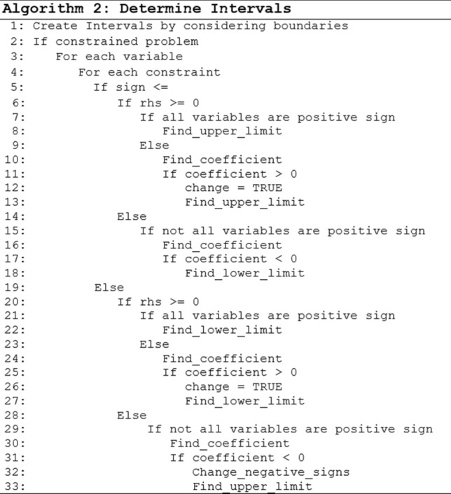

In essence, this approach adopts a principle of searching for the roots of each constraint in light of existing boundaries. This process continues until all constraints are evaluated. Through the process, many potential boundaries are calculated. However, at the end, the minimum values of upper limits and the maximum values of lower limits that satisfy all constraints are determined as final interval values for each variable.

Initialization

In this step, an initial solution set is generated concerning equal chances according to the determined intervals of variables in the hyperspace with multi-dimensions as much as the number of variables in the optimization model. To some extent, this method has been inspired by the “Scatter Search Algorithm” by Glover [53]. The approach for generating random numbers is proposed by Erdem [52], and then applied recently in [54]. The pseudocode is given below: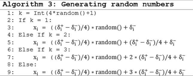

where ${\delta }_i^{-}$, ${\delta }_i^{+}$ are lower and upper limits, respectively; ${\mathrm{x}}_i$ is a generated random number for ith variable, and random () is defined as a function that generates a random number between [0,1].

The initialization step also includes the evaluations of constraints for each candidate solution vector. The solutions generated randomly are tested to whether they satisfy each constraint or not. The evaluation is conducted to calculate the constraint satisfaction rates and the total deviations. Therefore, a low satisfaction rate and significant deviations have resulted in big penalties in fitness values. This part will be handled in detail under the title of Multiplicative Penalty-based Method (MUPE).

PbA is structured as a memory-based algorithm. Although there are different approaches in the literature to use memory, “Tabu Search” and “Elitism Principle” are the pioneers of these approaches. For this reason, these approaches inspired the memory feature of the PbA. The PbA utilizes memory for two purposes. The first one is creating a database where each solution is recorded in a memory along with the evaluation scores (constraint satisfaction rates, total deviations). This procedure is inspired by the principle that each step in the “Tabu Search” algorithm is kept in a "history" mechanism, and the repetition of previous solutions is prohibited by looking at this memory [55]. However, in the PbA, memory is used not as a banned list but to eliminate unnecessary repetitive function evaluations. The second one is about recording the best-so-far positions of the solutions. This approach is inspired by the “Elitism Principle” in the literature. The elitism principle is the selection technique that saves the best solution in the population to eliminate the risk of losing the best solution between iterations [56]. In the PbA, best-so-far solutions are stored to avoid losing them in case of offsets. However, there are no limitations for the number of elitist solutions differently from the original elitism principle. Namely, the best-so-far solutions are kept separately from the relocated solution set.

Multiplicative penalty-based method (MUPE)

Penalty functions are the most common approaches in the constrained optimization literature for decades [57]. Penalty approaches are utilized to keep violations and feasibility under control by penalizing [58]. The penalty approach developed for the PbA is motivated by the studies [59–63]. The multiplicative penalty-based constraint handling (MUPE) method, firstly proposed by Erdem [52], calculates fitness function by considering satisfied constraints rate and deviations from constraints besides objective function in a multiplicative manner. In the case of unconstrained/bounded problems, the goal function would be the objective function itself. The pseudocode for the calculation of the heuristic fitness function is given below: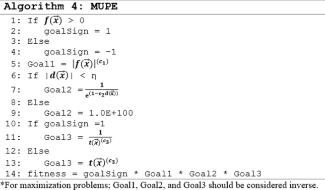

Herein goal function combines both the objective function and all constraints. The goal function acts as a heuristic function as shown below:

$$H\left(\overrightarrow{x}\right)=H(f\left(\overrightarrow{x}\right),d\left(\overrightarrow{x}\right),t\left(\overrightarrow{x}\right))$$ 1

where, $f\left(\overrightarrow{x}\right)$ represents Goal 1 which includes an objective function to be minimized/maximized, $d\left(\overrightarrow{x}\right)$ shows the total amount of violations of the constraints, and this function is controlled by Goal 2, $t\left(\overrightarrow{x}\right)$ is the ratio of the satisfied constraints which is represented by Goal 3, and finally $H\left(\overrightarrow{x}\right)$ corresponds to the fitness value of a candidate solution. Here Goal 2 and Goal 3 provide a benchmarking because two infeasible solution points have different constraint violation levels. Goal 2 deals with the total amount of violations measure for solutions. On the other hand, Goal 3 incorporates the ratio of satisfied constraints among overall ones. It can be concluded that selecting the “a solution point that has great violation on a single constraint, but the others satisfied” against “a solution point that has little violations for all the constraints” is a benchmarking interest of this method. If all of the constraints were satisfied for the two solution points, Goal 1 would be the only criteria for comparing these solution points.

This multi-objective function structure could have an acceptable convergence by violating constraints within defined precision. It is worth emphasizing that each goal is considered according to different importance scores, namely scores (c₁, c₂, c₃). The sign of the objective function is also added multiplicatively depending on whether the objective function is more significant than zero or not.

Offset factor

In the initialization part, the solutions are randomly assigned values, and then they start to reach better solutions. In PbA, an offset factor represents the relationship between a candidate solution vector and its neighbors. The offset factor exerted on each solution employs Eq. (2) where $H(\overrightarrow{x_i})$ correspond to the fitness values of candidate solutions and are calculated as below:

$$F=C\frac{H(\overrightarrow{x_i})H(\overrightarrow{x_l})}{d_{\mathit{il}}^2}$$ 2

where F is an offset factor between i and l solution vectors; C is a constant; $H\left(\overrightarrow{x_i}\right),H(\overrightarrow{x_l})$ are the fitness values of solutions i and l, respectively; d_il is the Euclidean distance between the solution vectors and the calculation is demonstrated below:

$$d_{\mathit{il}}=\sqrt{\sum _1^n{{(x}_{\mathit{in}}-x_{\mathit{ln}})}^2}=\sqrt{{(x_{i1}-x_{l1})}^2+{(x_{i2}-x_{l2})}^2+\cdots +{(x_{\mathit{in}}-x_{\mathit{ln}})}^2}$$ 3

After calculating the fitness values of each solution vector, the offset factor caused by the neighbors exerted on that solution is considered to find the new solution point. In the PbA, each solution is exposed to that factor from the closest solution vectors in the population by considering the neighborhood principle.

Neighborhood

The determination of the number of neighbors is also another critical issue to be addressed. According to Pareto’s Principle, roughly 80% of the effects come from 20% of the causes [63]. This principle corresponds that when neighborhood vectors are sorted in descending order, the magnitudes of the offset factors decrease sharply after the 2nd–5th vectors. For that reason, the rest of the solutions can be ignored in terms of fitness values. In the PbA, it is thought that the two closest neighbors may have the potential power for each solution to change its fitness value. Thus, these neighbors are utilized for the displacement procedure of the potential solution.

Offsetting

After identifying neighbors, the change in each solution must be calculated as a result of the offset factor. After all the factors exerted on the selected solution $\overrightarrow{x_i}$, the unified (or compound) net change is calculated, and the new solution is determined. The first iteration is completed after all the factors from neighbors are considered for each solution vector. Algorithm 5 shows the procedure of neighbors affects the solution until a net force is balanced.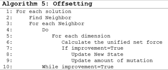

After the offset factors exerting on a solution, the unit offsetting can be found by Eq. (4). The amount of change for a related solution would be proportional to the related dimensional factor and its fitness function value as shown below:

$$\mathrm{\Delta }{x}_i^{{}^{\prime }}=\frac{F\frac{\mathrm{\Delta }{x}_i^2}{d^2}}{H(x_i)}=\frac{F}{H(x_i)}\frac{\mathrm{\Delta }{x}_i^2}{d^2}$$ 4

After considering all offset factors, each solution has a new fitness value in both magnitude and direction. In addition to the neighbors' effects on the related solution, the best-so-far solution also affects the corresponding solution. The new value is determined by the weighted impact of the neighbors and the best-so-far solution. The determination of the new solution is given in Eq. (5).

$$x_i^k=x_i^{k-1}+[\mathrm{\Delta }{x}_i^{k-1}\alpha +x_b^{k-1}\left(1,-,\alpha \right)],i=1,2,..,n$$ 5

where n is the number of dimensions, k is the iteration number, $\alpha ϵ\left[0,,,1\right]$, and it is a dynamic parameter based on the improvement within loops, and $x_b^{k-1}$ is the best-so-far solution. Here $\alpha$ provides an opportunity to control the balance between the neighbors and the best-so-far solution.

In line with the net offset factor, the solutions are exposed; they can change their fitness values if it has a better value, as shown in Eq. (6) for minimization problems. In case of having worse fitness value, the solution retains its current value by preserving the best-so-far solution in the population as in Elitism selection. It would be better to clarify that solution can be changed within the allowed space, determined by the intervals of variables.

$$H\left(x_i^k\right)<H\left(x_i^{k-1}\right)$$ 6

Furthermore, it is essential to clarify that if the new fitness value is out of boundaries, the new solution vector is updated as the boundary. When all offset factors are determined for each solution in the population, the first iteration is completed. These process chains are repeated until no remarkable factor from neighbors occurs. However, if a candidate solution is still under the effect of the offset factor, it changes its current value as a small increased amount of offsetting, as shown in Eq. (7).

$$\mathrm{\Delta }{x}_i^k=\mathrm{\Psi }\mathrm{\Delta }{x}_i^{k-1}$$ 7

where $\mathrm{\Psi }\in [1.01,1.1]$ and a subjective parameter. In case of improvements $\mathrm{\Delta }{x}_i^{k-1}$ continues to be multiplied by $\mathrm{\Psi }$. After considering all the factors caused by the neighbors, the unified net change is checked lastly and in case of remarkable change, new solution vectors are determined.

Duplication

As a diversification procedure, the PbA applies a procedure that two solution vectors cannot occupy the same fitness value in a closed system. Thus, solutions can diversify without trapping into a single point. Our experiments assume that fitness values are the same in the case that the first six decimal places are equal. In this step, the solution set is checked whether there is a duplicated solution or not. Thus, it is aimed that the algorithm does not trap into a local optimum by increasing the solution possibilities in the population.

While duplication check provides diversification, offsetting in a wide range can create too much diversity disrupting the balance. For this reason, the purpose of offsetting around the best-known solution is to balance the exploration–exploitation ability of the PbA.

Stopping condition

The stopping condition is related to the number of function evaluations (FES). The pseudocode for the stopping condition is given below. However, the algorithm will stop in most cases where the main stopping condition is met. The minimum, the maximum, and the average FES values are also reported for each problem.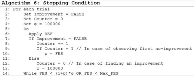

An illustrative example

In this section, an example is generated to explain the procedure of the proposed algorithm step by step including the most critical issues. The visualization is exemplified through fitness values and the minimization problem as shown in Fig. 2. The demonstration includes 4 crucial issues A. Initial Solution, B. Neighborhood, C. Offsetting, D. Best-so-far effect in the run, respectively. Each step is explained in the following.

Fig. 2.

An illustration of the PbA

The determination of the search space is the first step of PbA. At this stage, firstly the boundaries of the variables are considered as default, and then the boundaries are updated according to the root value of each constraint in case of having constraints, and the final search space is revealed. After the preliminary preparation is completed, a random initial solution is generated as shown in Algorithm 3 and A section in Fig. 2. The next steps include the efforts to reach a better point in line with the neighborhood relations of the population elements in the initial solution and the relationship between the best-so-far solution (denoted as black) in that solution. In Fig. 2, all steps are visualized over a single solution value denoted red. The neighborhood step identifies the two closest neighbors (denoted as yellow) that may have the potential power for the red solution to change its fitness value. The closeness of the neighbors is considered as the Euclidean distances. Through the offset factors of the neighbors, the red solution will try to reach a better point as shown in section C. The amount of change in its place is calculated with the help of Algorithm 5. Improvement efforts for better solutions are not limited to offset factors of neighbors. Besides, the best-so-far solution in that run also has a certain effect (1 − α) as mentioned in Eq. (5) including the neighbors’ effect (α). Consequently, the red solution takes its new position as shown in section D. It would be better to clarify that these procedures have been applied in case of having better fitness values; otherwise, the solution retains its current position. The first iteration is completed when new solution values are calculated for each solution in the population. These chains of processes are repeated until there is no appreciable offsetting from the neighbors and the best-so-far solution effect.

Constrained engineering optimization problems

According to Ezugwu et al. [65], the strength of the metaheuristics can be shown by the application in engineering design, management, industries, finance, and scheduling. This situation attracts the scientific community and industry practitioners. In general, before proposing a new algorithm, it is required to test its performance with appropriate test benchmarks [66].

The highlight of the PbA is the ability to deal with constraints very well because of the multiplicative penalty method. For this reason, the performance of the algorithm is evaluated with the most frequently used engineering benchmark problems (Pressure Vessel, Welded Beam, Tension/Compression Spring Design, Himmelblau’s Function), which may have complex constraints. In addition, although these benchmarks are referred to as engineering design problems in the literature, problems that are essentially aimed at "cost minimization.” The parameters used in the PbA are determined as a result of a trial-and-error test and presented in Table 2.

Table 2.

Parameter Settings

The number of trials	30
The importance scores (c1, c2, c3) (MUPE)	(0.25, 0.2, 1.8)
The number of the particles (population size) (n)	20
The incremental parameter ($\mathrm{\Psi }$)	1.02
The stopping parameter (β)	0.5*
The neighborhood size (κ)	2
The precision number (ρ)	6
Maximum number of Function Evaluations (Max FES)	30,000**

*1.5

**100,000 for Welded Beam

In general, the algorithms to which the developed algorithm will be compared are randomly selected and re-run and reported independently from the scholars who developed the algorithm. However, this situation may cause manipulation by using different parameters, different software hardware, or even different programming languages, giving biased results. For this reason, it will be better to compare the developed algorithm with the results of other algorithms as reported in the literature. At this point (if specified), the population size, the number of iterations, or the function evaluation value will be good indicators for comparison. Since the main purpose is to reach the best-known solutions so far or a better solution than the best-known, the algorithms developed, especially in recent years presented in Table 3, have been preferred for comparison.

Table 3.

Parameters used for algorithms published in the literature

Algorithm	Population	Max iteration	Trial	FES
Charged System Search (CSS) [29]	NA	NA	30	NA
Firefly Algorithm (FA) [67]	25	1000	NA	50,000e
Ray Optimization (RO) [68]	40	NA	50	NA
Magnetic Charged System Search (MCSS) [50]	NA	NA	30	NA
Cuckoo search algorithm (CSA) [69]	25	NA	NA	5000
Advanced particle swarm-assisted genetic algorithm (PSO-GA) [70]	NA	NA	30	5000
Artificial Bee Colony Algorithm (ABC) [71]	20*D	500	30	NA
Plant Propagation Algorithm (PPA) [72]	40	25	100	30,000
Hybrid Flower Pollination Algorithm (H-FPA) [73]	50	1000	30	NA
Modified Oracle Penalty Method (MOPM) [74]	30	NA	100	90,000
Interior Search Algorithm (ISA) [75]	NA	NA	30	30,000*
Grey Wolf Optimizer (GWO) [76]	NA	NA	NA	NA
Optics Inspired Optimization (OIO) [77]	19	NA	30	5000
Hybrid PSO-GA Algorithm (H-PSO-GA) [78]	20*D	NA	30	NA
Thermal Exchange Optimization (TEO) [79]	30	10,000	30	NA
Seagull Optimization Algorithm (SOA) [80]	100	1000	30	NA
Pathfinder algorithm (PA) [81]	60	100	NA	NA
Hybrid GSA-GA Algorithm (H-GSA-GA) [82]	20*D	200	30	NA
Nuclear Fission-Nuclear Fusion Algorithm (N2F) [83]	40	NA	30	30,000
Marine Predators Algorithm (MPA) [84]	NA	500	30	25,000
Equilibrium Optimizer (EO) [85]	30	500	NA	15,000
Search and Rescue Optimization Algorithm (SRO) [86]	20	NA	50	30,000a
Chaotic Grey Wolf Optimizer (CGWO) [87]	100	NA	30	40,000
Slime Mould Algorithm (SMA) [88]	NA	NA	NA	NA
Chaos Game Optimization (CGO) [89]	NA	NA	25	NA
Group Teaching Optimization Algorithm (GTO) [90]	50	NA	30	10,000
Teaching–Learning-based Marine Predator Algorithm (TLMPA) [91]	NA	NA	30	NA
Smell Bees Optimization Algorithm (SBO) [92]	NA	NA	50c	14,000b
Improved Grey Wolf Optimizer (IGWO) [93]	20	(D*104)/20d	10	NA
Cooperation Search Algorithm (CoSA) [94]	50	1000	20	NA
Hybrid Social Whale Optimization Algorithm (HS-WOA) [95]	50	NA	30	NA
Hybrid Social Whale Optimization Algorithm (HS-WOA +) [95]	25	NA	30	NA
Atomic Orbital Search (AOS) [96]	NA	NA	25	200,000
Lichtenberg Algorithm (LA) [97]	100	200	30	NA
Dingo Optimization Algorithm (DOA) [98]	100	500	30	NA
Material Generation Algorithm (MGA) [99]	NA	NA	25	20,000*D
Rat Swarm Optimizer (RSO) [100]	30	1000	NA	NA
Colony Predation Algorithm (CPA) [101]	30	NA	30	1000
Sand Cat Swarm Optimization (SCSO) [102]	30	500	30	NA
Archerfish Hunting Optimizer (AHO) [103]	30*s1.5	200,000/(30*s1.5)	25	NA

*5000 for pressure/8900 for Tension Compression Spring Design

**s is the search space

^a15,000 for Welded Beam/25000 for Tension/Compression Spring Design

^b13,000 for Tension/Compression Spring Design and Welded Beam

^c30 for Welded Beam

^dD is the number of variables

^e25,000 for Pressure Vessel

In the comparison tables for each problem, six decimal places are documented if reported. The results obtained by the PbA are also presented with the same sensitivity. Moreover, we preferred to code the PbA in Python language by utilizing Python libraries and PyCharm [104]. The experiments are executed on an Intel Core i7 computer with a 2.60 GHz CPU and 12 GB RAM under the windows operating system.

In the following sections, the experimental results for Pressure Vessel, Welded Beam, Tension/Compression Spring Design, and Himmelblau’s Function are presented in detail.

Pressure Vessel

The design of a Pressure Vessel is one of the most used cost optimization problems. The design image of the vessel is given in Fig. 3. This problem has four variables where x₃ and x₄ are continuous, while x₁ and x₂ are integers (products of 0.0625 inches) which are the available thickness of the material.

Fig. 3.

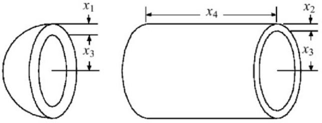
Pressure Vessel [105]

The model of the Pressure Vessel is given below:

$$\begin{array}{c}\text{Minimize}f\left(\overrightarrow{x}\right)=0.6224x_1{x}_3{x}_4+1.7781x_2{x}_3^2+3.1661x_1^2{x}_4+19.84x_1^2{x}_3\\ \text{Subject}\text{to}\\ g_1\left(\overrightarrow{x}\right)=-x_1+0.0193x_3\le 0\\ g_2\left(\overrightarrow{x}\right)=-x_2+0.00954x_3\le 0\\ g_3\left(\overrightarrow{x}\right)=-\pi x_3^2{x}_4-\frac{4}{3}\pi x_3^3+1296000\le 0\\ x_1,x_2\in \left[0.0625,10\right];x_3\in \left[0,100\right];x_4\in \left[0,240\right]\\ \end{array}$$ 8

It would be useful to show how the proposed algorithm handles a problem step by step and arrives at a near-optimal result before reporting the final solutions for each problem. The convergence process of the PbA is exemplified for Pressure Vessel in Table 4. The other engineering design problems converge similarly.

Table 4.

Convergence of the proposed algorithm

	Best-so-far solution
	x1	x2	x3	x4	Objective value
1st Iteration	0.75	3.6875	38.3180537	233.2875928	14,642.97428
2nd Iteration	0.75	0.5	38.8336281	222.377235	6201.305994
50th Iteration	0.75	0.375	38.85927662	221.3822673	5850.58009901902
150th Iteration	0.75	0.375	38.85987911	221.369303	5850.4220474207
.	.	.	.	.	.
246th Iteration	0.75	0.375	38.8601	221.3655	5850.38306

The experimental results for Pressure Vessel are summarized in Table 5 as descriptive statistics. Although maximum FES is limited to 30,000, actual FES values are also reported as well.

Table 5.

Experimental results of Pressure Vessel

Best	5850.38306	Average iteration	163.63
Mean	6659.547045	Minimum FES	2527
Worst	7903.694033	Average FES	20,002.3
Standard deviation	713.15	Maximum FES	30,091
Standard error	130.2

The best-so-far solution for the Pressure Vessel obtained by the PbA is given in Table 6. Moreover, the left-hand side values of each constraint are also provided in Table 6 to show the feasibility of the solution.

Table 6.

Best-so-far solution for Pressure Vessel

Objective	x1	x2	x3	x4
5850.38306	0.75	0.375	38.860104	221.365471
Constraints	g1(x)	g2(x)	g3(x)
	− 3.24056E-11	− 0.004275	− 2.41133E-05

In Fig. 4 a graphic is given in order to show the convergence to the global minimum of the algorithm visually. It shows the objective function values obtained according to the FES value in the related run reaching the global minimum within 30 trials. As it is seen, the best-so-far solution has been reached approximately after 5000 function evaluations.

Fig. 4.

The convergence to the best-so-far solution (pressure vessel)

The Pressure Vessel problem has been handled with many other metaheuristic algorithms previously. Since there are too many algorithms in the literature, only those developed after 2010 are presented chronologically in Table 7. Most of the solutions could not be able to satisfy “having x₁ and x₂ as integer products of 0.0625.” The feasible best-known solution for Pressure Vessel has been obtained firstly by FA. However, there are no other algorithms that reach this solution. PbA has provided the same best-known solution with a smaller set size compared to FA.

Table 7.

Comparisons for pressure vessel (Best-so-far solution)

Algorithm	× 1	× 2	× 3	× 4	Objective
CSS [28]	0.8125	0.4375	42.103624	176.572656	6059.09
FA [63]	0.75	0.375	38.8601	221.36547	5850.38306
MCSS [49]	0.8125	0.4375	42.10455	176.560967	6058.97
MOPM [70]	0.8125	0.4375	42.098446	176.636596	6059.7143
ISA [71]	0.8125	0.4375	42.09845	176.6366	6059.7143
GWO [72]	0.8125	0.4345	42.089181	176.758731	6051.5639
TEO [75]	0.779151	0.385296	40.369858	199.301899	5887.511073
SOA [76]	0.77808	0.383247	40.31512	200	5879.5241
PA [77]	0.778168	0.384649	40.31964	199.9999	5885.3351
N2F [79]	1.125	0.625	58.290155	43.6926562	7197.72893
MPA [80]	0.8125	0.4375	42.098445	176.636607	6059.7144
EO [81]	0.8125	0.4375	42.098446	176.636596	6059.7143
SRO [82]	0.8125	0.4375	42.098446	176.636596	6059.714335
SMA [84]	0.7931	0.3932	40.6711	196.2178	5994.1857
CGO [85]	0.778169	0.51	40.319619	200	6247.672819
GTO [86]	0.778169	0.38465	40.3196	200	5885.333
TLMPA [87]	0.778169	0.384649	40.319618	200	5885.332774
SBO [88]	0.778169	0.384649	40.319619	199.999999	5885.33262
IGWO [89]	0.779031	0.385501	40.36313	199.4017	5888.34
HS-WOA + [95]	0.778168	0.384649	40.319622	199.999953	5885.331515
HS-WOA [95]	0.778486	0.385076	40.326495	199.998992	5889.976089
AOS [96]	0.778674	0.385322	40.340891	199.721518	5888.457948
DOA [98]	0.8125	0.4375	42.09845	176.6366	6059.7143
MGA [99]	NA	NA	NA	NA	6059.714350
RSO [100]	0.775967	0.383127	40.313297	200	5878.5395
CPA [101]	0.81250	0.437500	42.088230	176.763300	6060.9590
SCSO [102]	0.7798	0.9390	40.3864	199.2918	5917.46
AHO [103]	NA	NA	NA	NA	6060
Proposed algorithm (PbA)	0.75	0.375	38.860104	221.365471	5850.38306

The descriptive statistics of the experiments are shown in Table 8. As it is seen, the performance of the PbA is better than the solutions reached by other algorithms. Although the worst and the standard deviation are relatively higher than the others, the feasible best-known solution is obtained by the PbA.

Table 8.

Comparisons for pressure vessel (descriptive statistics)

Algorithm	Best	Mean	Worst	Std Dev
CSS [28]	6059.09	6067.91	6085.48	10.2564
FA [63]	5850.38306	NA	NA	NA
MCSS [49]	6058.97	6063.18	6074.74	9.73494
MOPM [70]	6059.7143	6059.7143	6059.7143	1.94E-08
ISA [71]	6059.714	6410.087	7332.846	384.6
GWO [72]	6051.5639	NA	NA	NA
TEO [75]	5887.511073	5942.565917	6134.187981	62.2212
SOA [76]	5879.5241	5883.0052	5893.4521	256.415
PA [77]	5885.3351	NA	NA	NA
N2F [79]	7197.72893	7197.72905	7197.72924	7.90E-05
MPA [80]	6059.7144	6102.8271	6410.0929	106.61
EO [81]	6059.7143	6668.114	7544.4925	566.24
SRO [82]	6059.714335	6091.32594	6410.0868	8.03E + 01
SMA [84]	5994.1857	NA	NA	NA
CGO [85]	6247.672819	6250.957354	6330.958685	10.75915635
GTO [86]	5885.333	NA	NA	NA
TLMPA [87]	5885.332774	NA	NA	NA
SBO [88]	5885.33262	6156.4028	6384.8583	74.9635
IGWO [89]	5888.34	NA	NA	NA
HS-WOA + [95]	5885.332	5906.331	5998.331	72.1541
HS-WOA [95]	5889.976	5946.629	6231.362	121.0098
AOS [96]	5888.457948	5888.480501	5894.840682	2.199072
DOA [98]	6059.7143	NA	NA	NA
MGA [99]	6059.714350	6059.694923	6273.765974	0.028912
RSO [100]	5878.5395	5881.5355	5887.3933	167.041
CPA [101]	6060.9590	NA	NA	NA
SCSO [102]	5917.46	NA	NA	NA
AHO [103]	6060	7330	6150	6.25
Proposed Algorithm (PbA)	5850.383	6659.547045	7903.694	713.15

Welded Beam

The Welded Beam is a structural optimization problem generally preferred as a benchmark [106]. This structure is about the beam and the weld for mass production, as shown in Fig. 5. This cost optimization problem consists of four design variables and six constraints. The model is given in Eq. 9.

$$\begin{array}{c}\text{Minimize}f\left(\overrightarrow{x}\right)=\left(1+c_1\right)x_1^2{x}_2+c_2{x}_3{x}_4\left(L+x_2\right)\\ \text{Subject}\text{to}\\ g_1\left(\overrightarrow{x}\right)=\tau \left(\overrightarrow{x}\right)-{\tau }_{\text{max}}\le 0\\ g_2\left(\overrightarrow{x}\right)=\sigma \left(\overrightarrow{x}\right)-{\sigma }_{\text{max}}\le 0\\ g_3\left(\overrightarrow{x}\right)=x_1-x_4\le 0\\ g_4\left(\overrightarrow{x}\right)=c_1{x}_1^2+c_2{x}_3{x}_4\left(L+x_2\right)-5\le 0\\ g_5\left(\overrightarrow{x}\right)=\delta \left(\overrightarrow{x}\right)-{\delta }_{\text{max}}\le 0\\ g_6\left(\overrightarrow{x}\right)=P-P_c\left(\overrightarrow{x}\right)\le 0\\ \tau \left(\overrightarrow{x}\right)=\sqrt{{\left({\tau }^{\prime }\right)}^2+2{\tau }^{\prime }{\tau }^{″}\frac{x_2}{2R}+{({\tau }^{″})}^2}\\ {\tau }^{\prime }=\frac{P}{\sqrt{2}{x}_1{x}_2};{\tau }^{″}=\frac{\mathit{MR}}{J};M=P\left(L+\frac{X_2}{2}\right);R=\sqrt{\frac{x_2^2}{4}+{\left(\frac{x_1+x_3}{2}\right)}^2}\\ J=2\left\{\sqrt{2}{x}_1{x}_2\left[\frac{x_2^2}{12}+{\left(\frac{x_1+x_3}{2}\right)}^2\right]\right\}\\ \sigma \left(\overrightarrow{x}\right)=\frac{6PL}{x_4{x}_3^2};\delta \left(\overrightarrow{x}\right)=\frac{4P{L}^3}{E{x}_3^3{x}_4}\\ P_c\left(\overrightarrow{x}\right)=\frac{4.013E\sqrt{\frac{x_3^2{x}_4^6}{36}}}{L^2}\left(1-\frac{x_3}{2L}\sqrt{\frac{E}{4G}}\right)\\ x_1\in \left[0.125,5\right];x_2,x_3\in \left[0.1,10\right];x_4\in \left[0.1,5\right]\\ {\text{c}}_1=0.10471;{\text{c}}_2=0.04811;\text{P}=6000;\text{L}=14;\text{E}=30000000;\text{G}=12000000\\ {\delta }_{\text{max}}=0.25;{\tau }_{\text{max}}=13600;{\sigma }_{\text{max}}=30000\\ \end{array}$$ 9

Fig. 5.

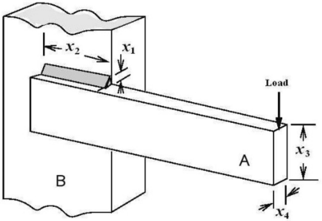
Welded beam [105]

The experimental results for Welded Beam are given in Table 9 as descriptive statistics. Only for Welded Beam problem, maximum FES is limited to 100,000, and actual FES values are also reported as well.

Table 9.

Experimental results of Welded Beam

Best	1.724872	Average iteration	741.53
Mean	1.799315	Minimum FES	47,257
Worst	2.278059	Average FES	89,236.7
Standard deviation	0.12	Maximum FES	100,126
Standard error	0.02

The best-so-far solution for Welded Beam obtained by the PbA is given in Table 10. Furthermore, to show the feasibility of the solution, each constraint's left-hand side values are also provided. As seen from the constraint values, only one constraint has a 2.96612E-07 violation which is negligible. Therefore, it can be concluded that the solution is feasible as well.

Table 10.

Best-so-far solution for welded beam

Objective	x1	x2	x3	x4
1.724872	0.205715	3.470808	9.036624	0.20573
Constraints	g1(x)	g2(x)	g3(x)
	− 3.1307E-06	2.96612E-07	− 1.48238E-05
	g4(x)	g5(x)	g6(x)
	− 3.390637	− 0.23554	− 0.001607

In Fig. 6, a graphic is given to show the convergence to the global minimum of the algorithm visually. Figure 6 shows the objective function values obtained according to the FES value in the run reaching the global minimum within 30 trials. The algorithm has converged the best-so-far solution after 30,000 FES, according to the graph.

Fig. 6.

The convergence to the best-so-far solution (Welded Beam)

The feasible best-known solution for Welded Beam has been obtained as 1.724852 in the literature. Most of the algorithms have reached feasible best-known solutions. However, the solution values obtained differ after the 5th digit after the comma, as shown in Table 11. It is worth noting that the solutions less than 1.724852 are infeasible for some constraints.

Table 11.

Comparisons for Welded Beam (Best-so-far solution)

Algorithm	× 1	× 2	× 3	× 4	Objective
CSS [28]	0.20582	3.468109	9.038024	0.205723	1.724866
FA [67]	0.2015	3.562	9.0414	0.2057	1.73121
RO [68]	0.203687	3.528467	9.004233	0.207241	1.735344
MCSS [50]	0.20573	3.470489	9.036624	0.20573	1.724855
MOPM [74]	0.20573	3.470489	9.036624	0.20573	1.724852
ISA [75]	0.244330	6.219931	8.291521	0.244369	2.3812
GWO [76]	0.205676	3.478377	9.03681	0.205778	1.72624
TEO [79]	0.205681	3.472305	9.035133	0.205796	1.725284
SOA [80]	0.205408	3.472316	9.035208	0.201141	1.723485
PA [81]	0.02058	3.470495	9.036624	0.20573	1.724853
N2F [83]	0.20573	3.470489	9.036624	0.20573	1.724852
MPA [84]	0.205728	3.470509	9.036624	0.20573	1.724853
EO [85]	0.2057	3.4705	9.03664	0.2057	1.7549
SRO [86]	0.20573	3.470489	9.036624	0.20573	1.724852
CGWO [87]	0.20573	3.470499	9.036637	0.20573	1.724854
SMA [88]	0.2054	3.2589	9.0384	0.2058	1.69604
CGO [89]	0.198856	3.337244	9.191454	0.198858	1.670336
GTO [90]	0.20573	3.470489	9.036624	0.20573	1.724852
TLMPA [91]	0.20573	3.470489	9.036624	0.20573	1.724852
SBO [92]	0.175055	3.305377	9.248898	0.206137	1.699215
IGWO [93]	0.20573	3.47049	9.036624	0.20573	1.724853
CoSA [94]	0.205692	3.254453	9.03636	0.205733	1.695505
HS-WOA + [95]	0.20573	3.470489	9.036624	0.20573	1.724852
HS-WOA [95]	0.208079	3.442723	8.986502	0.208651	1.738146
AOS [96]	0.205730	3.470489	9.036624	0.205730	1.724852
LA [97]	0.2213	3.2818	8.7579	0.2216	1.8446
MGA [99]	NA	NA	NA	NA	1.672967
RSO [100]	0.205397	3.465789	9.034571	0.201097	1.722789
CPA [101]	0.188500	3.562000	9.134835	0.205245	1.723916
SCSO [102]	0.2057	3.2530	9.0366	0.2057	1.6952
AHO [103]	NA	NA	NA	NA	1.67
Proposed algorithm (PbA)	0.205715	3.470808	9.036624	0.20573	1.724872

In Table 12, the descriptive statistics for Welded Beam are reported. Table 12 indicates that the PbA achieves the best-known solution nearly (with a 2.04E-05 deviation, which is negligible).

Table 12.

Comparisons for Welded Beam (Descriptive Statistics)

Algorithm	Best	Mean	Worst	Std Dev
CSS [28]	1.724866	1.739654	1.759479	0.008064
FA [67]	1.73121	NA	NA	NA
RO [68]	1.735344	1.9083	NA	0.173744
MCSS [50]	1.724855	1.735374	1.750127	0.007571
MOPM [74]	1.724852	1.7249	1.749	1.11E-08
ISA [75]	2.3812	2.4973	2.67	1.02E-01
GWO [76]	1.72624	NA	NA	NA
TEO [79]	1.725284	1.76804	1.931161	0.058166
SOA [80]	1.723485	1.724251	1.727102	1.724007
PA [81]	1.724853	NA	NA	NA
N2F [83]	1.724852	1.725	1.726147	3.39E-04
MPA [84]	1.724853	1.724861	1.724873	6.41E-06
EO [85]	1.724853	1.726482	1.736725	0.003257
SRO [86]	1.724852	1.724852	1.724852	2.22E-11
CGWO [87]	1.724854	1.724854	1.724854	3.36E-16
SMA [88]	1.69604	NA	NA	NA
CGO [89]	1.670336	1.670378	1.670903	9.30E-05
GTO [90]	1.724852	NA	NA	NA
TLMPA [91]	1.724852	NA	NA	NA
SBO [92]	1.699215	1.719856	1.743486	0.014826
IGWO [93]	1.724853	NA	NA	NA
CoSA [94]	1.695505	1.724051	1.873922	0.047618
HS-WOA + [95]	1.724852	1.754853	1.848521	0.000249
HS-WOA [95]	1.738146	1.739235	1.948905	0.001349
AOS [96]	1.724852	1.725674	1.732516	0.024787
LA [97]	1.7351	1.8446	NA	0.1597
MGA [99]	1.672967	1.678791	1.687172	4.41E-03
RSO [100]	1.722789	1.725097	1.726987	0.015748
CPA [101]	1.723916	NA	NA	NA
SCSO [102]	1.6952	NA	NA	NA
AHO [103]	1.67	1.67	1.67	1.15E-14
Proposed Algorithm (PbA)	1.724872	1.799315	2.278059	0.12

Tension/Compression Spring Design

The Tension/Compression Spring Design Problem is an optimization benchmark that minimizes the weight [107]. There are three variables and four constraints. Its figure and model are given in Fig. 7 and Eq. 10, respectively.

$$\begin{array}{c}\text{Minimize}f\left(\overrightarrow{x}\right)=\left(x_3+2\right)x_2{x}_1^2\\ \text{Subject}\text{to}\\ g_1\left(\overrightarrow{x}\right)=1-\frac{x_2^3{x}_3}{71785x_1^4}\le 0\\ g_2\left(\overrightarrow{x}\right)=\frac{4x_2^2-x_1{x}_2}{12566\left(x_2{x}_1^3-x_1^4\right)}+\frac{1}{5108x_1^2}-1\le 0\\ g_3\left(\overrightarrow{x}\right)=1-\frac{140.45x_1}{x_2^2{x}_3}\le 0\\ g_4\left(\overrightarrow{x}\right)=\frac{x_1+x_2}{1.5}-1\le 0\\ x_1\in \left[0.05,1\right];x_2\in \left[0.25,1.3\right];x_3\in \left[2,15\right]\\ \end{array}$$ 10

Fig. 7.

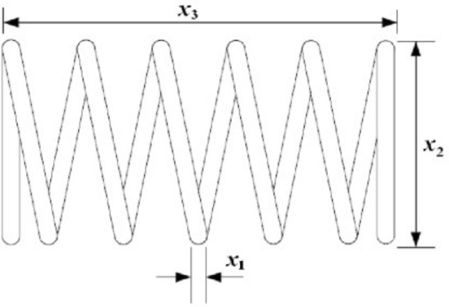
Tension/Compression Spring Design [105]

The experimental results for Tension/Compression Spring Design are given in Table 13 as descriptive statistics. Maximum FES is limited to 30,000, and the minimum and the average FES values are also reported as well.

Table 13.

Experimental results of Tension/Compression Spring Design

Best	0.012665	Average iteration	227.43
Mean	0.013404	Minimum FES	11,970
Worst	0.01705	Average FES	28,646.73
Standard deviation	0.0013	Maximum FES	30,120
Standard error	0.0002

The best-so-far solution for Tension/Compression Spring Design obtained by the PbA is given in Table 14. As is seen in Table 14, all constraints are satisfied.

Table 14.

Best-so-far solution for Tension/Compression Spring Design

Objective	x1	x2	x3
0.012665	0.05182	0.359887	11.105579
Constraints	g1(x)	g2(x)	g3(x)	g4(x)
	− 8.18448E-10	− 1.77694E-07	− 4.059998	− 0.725529

A graphic is given in Fig. 8 to visually express the algorithm's convergence to the global minimum value. It shows the objective function values obtained according to the FES value in the run reaching the global minimum within 30 trials. It is seen that the best-so-far solution has been obtained at the very beginning of FES values.

Fig. 8.

The convergence to the best-so-far solution (Tension/Compression Spring Design)

According to Table 15, the feasible best-known solution is 0.012665 reported in the literature. When the digits of the solutions reaching the value of 0.012665 are compared, it is evident that the PbA also reached the value of the best-known solution. It is worth noting that the solutions less than 0.012665 are infeasible to some extent.

Table 15.

Comparisons for Tension/Compression Spring Design (best-so-far solution)

Algorithm	× 1	× 2	× 3	Objective
CSS [28]	0.051744	0.358532	11.165704	0.012638
RO [68]	0.05137	0.349096	11.7679	0.012679
MCSS [50]	0.051627	0.35629	11.275456	0.012607
MOPM [74]	0.051718	0.357418	11.248016	0.012665
ISA [75]	NA	NA	NA	0.012665
GWO [76]	0.05169	0.356737	11.28885	0.012666
TEO [79]	0.051775	0.358792	11.16839	0.012665
SOA [80]	0.051065	0.342897	12.0885	0.012645
PA [81]	0.051727	0.35763	11.235724	0.012665
MPA [84]	0.051725	0.357570	11.239196	0.012665
EO [85]	0.05162	0.355054	11.387968	0.012666
SRO [86]	0.051689	0.356723	11.288648	0.012665
CGO [89]	0.051663	0.356078	11.326575	0.012665
TLMPA [91]	0.051681	0.356533	11.299823	0.012665
SBO [92]	0.051598	0.354523	11.418801	0.012665
HS-WOA + [95]	0.05192	0.362288	10.969723	0.012666
HS-WOA [95]	0.053446	0.399928	9.173312	0.012764
AOS [96]	0.051690	0.356729	11.288297	0.012665
MGA [99]	NA	NA	NA	0.012665
RSO [100]	0.051075	0.341987	12.0667	0.012656
CPA [101]	0.051741	0.357978	11.21548	0.012665
SCSO [102]	0.0500	0.3175	14.0200	0.012717
AHO [103]	NA	NA	NA	0.0127
Proposed Algorithm (PbA)	0.05182	0.359887	11.105579	0.012665

The descriptive statistics for Tension/Compression Spring Design are listed in Table 16. As it is seen, the performance of the PbA is better than the solutions reached by other algorithms.

Table 16.

Comparisons for Tension/Compression Spring Design (Descriptive Statistics)

Algorithm	Best	Mean	Worst	Std Dev
CSS [28]	0.012638	0.012852	0.013626	8.3564e−5
RO [68]	0.012679	0.013547	NA	0.001159
MCSS [50]	0.012607	0.012712	0.012982	4.7831e−5
MOPM [74]	0.012665	0.012665	0.012665	1.87E-08
ISA [75]	0.012665	0.013165	0.012799	1.59E-02
GWO [76]	0.012666	NA	NA	NA
TEO [79]	0.012665	0.012685	0.012715	4.41E-06
SOA [80]	0.012645	0.012666	0.012666	0.001108
PA [81]	0.012665	NA	NA	NA
MPA [84]	0.012665	0.012665	0.012665	5.55E-08
EO [85]	0.012666	0.013017	0.013997	3.91E-04
SRO [86]	0.012665	0.012665	0.012668	1.26E-07
CGO [89]	0.012665	0.012670	0.012719	1.09E-05
TLMPA [91]	0.012665	NA	NA	NA
SBO [92]	0.012665	0.012687	0.012723	1.77E-05
HS-WOA + [95]	0.012666	0.012745	0.012827	0.000105
HS-WOA [95]	0.012764	0.012816	0.012918	0.000121
AOS [96]	0.012665	0.012738	0.013597	0.000121
MGA [99]	0.012665	0.012666	0.012667	5.65E-07
RSO [100]	0.012656	0.012666	0.012668	0.057894
CPA [101]	0.012665	NA	NA	NA
SCSO [102]	0.012717	NA	NA	NA
AHO [103]	0.0127	0.0129	0.0151	2.17E-04
Proposed Algorithm (PbA)	0.012665	0.013404	0.01705	0.0013

Himmelblau’s Function

Himmelblau proposed a nonlinear constrained optimization problem in 1972, and it is regarded as a mechanical engineering problem [108]. This well-known problem has five variables and six constraints. The model of the problem is given in Eq. 11.

$$\begin{array}{c}\text{Minimize}f\left(\overrightarrow{x}\right)=5.3578547x_3^2+0.8356891x_1{x}_5+37.293239x_1-40792.141\\ \text{Subject}\text{to}\\ g_1\left(\overrightarrow{x}\right)=85.334407+0.0056858x_2{x}_5+0.00026x_1{x}_4-0.0022053x_3{x}_5\\ g_2\left(\overrightarrow{x}\right)=80.51249+0.0071317x_2{x}_5+0.0029955x_1{x}_2+0.0021813x_3^2\\ g_3\left(\overrightarrow{x}\right)=9.300961+0.0047026x_3{x}_5+0.0012547x_1{x}_3+0.0019085x_3{x}_4\\ 0\le g_1\left(\overrightarrow{x}\right)\le 92\\ 90\le g_2\left(\overrightarrow{x}\right)\le 110\\ 20\le g_3\left(\overrightarrow{x}\right)\le 25\\ x_1\in \left[78,102\right];x_2\in \left[33,45\right];x_3,x_4,x_5\in \left[27,45\right]\\ \end{array}$$ 11

The experimental results for Himmelblau’s Function are given in Table 17 as descriptive statistics. Maximum FES is limited to 30,000, and the minimum and the average FES values are also reported as well.

Table 17.

Experimental results of Himmelblau’s Function

Best	− 31,025.546836	Average iteration	171.5
Mean	− 30,986.343296	Minimum FES	4918
Worst	− 30,642.489379	Average FES	21,415.3
Standard deviation	94.38	Maximum FES	30,106
Standard error	17.23

The solution for Himmelblau’s Function obtained by the PbA is given in Table 18. As it is seen, all constraints are within the defined range, which means that there are no violations.

Table 18.

Best-so-far solution for Himmelblau’s Function

Objective	x1	x2	x3	x4	x5
− 31,025.546836	78	33	27.07115	44.999999	44.968769
Constraints	g1(x)	g2(x)	g3(x)
	91.999924	100.404691	20

In Fig. 9, a graphic is given in order to show the convergence of the algorithm to the global minimum visually. It shows the objective function values obtained according to the FES value in the run reaching the global minimum within 30 trials. According to Fig. 9, it is seen that the algorithm has achieved convergence of the best-so-far solution with less than 10,000 FES values.

Fig. 9.

The convergence to the best-so-far solution (Himmelblau)

In Table 19, the feasible best-known solutions obtained for Himmelblau’s Function are given. H-GSA-GA reaches the best-known solution with -31,027.64076. However, it would be better to mention that H-GSA-GA utilizes 20*Dimension as population size, which becomes 100.

Table 19.

Comparisons for Himmelblau’s Function (Best-so-far solution)

Algorithm	× 1	× 2	× 3	× 4	× 5	Objective
CSA [69]	78	33	29.99616	45	36.77605	− 30,665.233
PSO-GA [70]	78	33	29.99525	45	36.77582	− 30,665.5389
ABC [71]	78	33	27.07098	45	44.969024	− 31,025.57569
PPA [72]	78	33	29.9952	45	36.7758	− 30,665.54
H-FPA [73]	NA	NA	NA	NA	NA	− 31,025.5654
OIO [77]	NA	NA	NA	NA	NA	− 31,025.50178
H-PSO-GA [78]	78	33	27.070951	45	44.969167	− 31,025.57471
H-GSA-GA [82]	77.961	32.99948	27.072836	45	44.973943	− 31,027.64076
CSA [94]	78	33	29.995256	45	36.775813	− 30,665.538672
Proposed Algorithm (PbA)	78	33	27.07115	44.999999	44.968769	− 31,025.546836

The descriptive statistics for Himmelblau’s Function are listed in Table 20. As seen, the performance of the PbA for Himmelblau's Function is considerably good.

Table 20.

Comparisons for Himmelblau’s Function (Descriptive Statistics)

Algorithm	Best	Mean	Worst	Std Dev
CSA [69]	− 30,665.233	NA	NA	11.6231
PSO-GA [70]	− 30,665.5389	− 30,665.53697	− 30,665.48996	8.76E-03
ABC [71]	− 31,025.57569	− 31,025.55841	− 31,025.49205	0.015353
PPA [72]	− 30,665.54	NA	NA	NA
H-FPA [73]	− 31,025.5654	NA	NA	NA
OIO [77]	− 31,025.50178	− 31,024.5348	− 31,020.60517	1.2092
H-PSO-GA [78]	− 31,025.57471	− 31,025.55782	− 31,025.49205	0.01526
H-GSA-GA [82]	− 31,027.64076	− 31,026.07246	− 31,025.38705	0.01803
CSA [94]	− 30,665.538672	− 30,625.97242	− 30,561.19298	35.52345
Proposed Algorithm (PbA)	− 31,025.54684	− 30,986.3	− 30,642.48938	94.38

Discussion and conclusion

This study presents a new population-based evolutionary computation model for solving continuous constrained nonlinear optimization problems. The proposed algorithm assumes that candidate solutions in a defined search space are in interaction to survive through having better fitness values. The interaction between candidate solutions is limited with the closest neighbors by considering the Euclidean distance. The outstanding feature of the PbA is the MUPE which considers satisfied constraints rate and deviations from constraints besides objective function in a multiplicative manner. Another prominent feature in the PbA is the control mechanism for duplication, which is for satisfying Pauli’s Exclusion Principle in physics. PbA is structured as a memory-based algorithm inspired by Tabu Search and Elitism at some point. A database structure has been created to reduce the function evaluation load in the algorithm. This database can be thought of as a memory capability of the PbA. However, unlike in Tabu Search, this database is designed as a particle repository, not a banned list. On the other hand, the best solutions achieved are also recorded and kept separately. However, this does not include a specific ratio as in the Elitism approach; on the contrary, the best set is used as much as the population size. Although the PbA is inspired by natural facts and other algorithms in the literature, the primary goal is to achieve better results in a specific problem type, regardless of metaphors and similarities.

To show the performance of the PbA, the most common engineering design problems such as Pressure Vessel, Welded Beam, Tension Compression Spring Design, and Himmelblau’s Function are applied. The experimental studies have shown that the PbA performs well to handle constraints while minimizing objective functions, and the PbA has provided the best-known solutions in the literature. It should be pointed out that solution set size significantly impacts the results. For this reason, the PbA has been performed with the minimum set size listed in the comparison table. It is evident that, in the case of a more extensive set size, the best-known solutions can be reached more quickly in the PbA.

Limitations of this study should be noted as well. The performance of the proposed algorithm is limited by the real-world engineering design problems handled. Furthermore, parameter setting for importance scores in MUPE approach has been determined by trial and error which can be considered a disadvantage of the proposed algorithm. Apart from this, hardware qualifications such as central processing unit (CPU), computer data storage, and the motherboard can also be considered as limitations.

For further studies, different benchmark group problems (unconstrained, multi-objective, combinatorial, etc.) can be solved after some modifications of the PbA. Furthermore, the PbA can be integrated with other constraint handling methods. Modifications can achieve the desired result with less function evaluation value. It can be combined with various algorithms as a different hybrid algorithm. Moreover, as stated by Gambella et al. [109], the concept of optimization problems for machine learning presents novel research directions by considering machine learning models as complement approaches in addition to the existing optimization algorithms. For instance, the proposed algorithm can be implemented in any place where other evolutionary algorithms such as genetic algorithm have been utilized for itemset mining as shown in [110, 111]. Besides, it can be integrated with any deep learning algorithms to diagnose the disease as handled in [112].

Appendix

ABC	Artificial bee colony algorithm
AHO	Archerfish hunting optimizer
AOS	Atomic orbital search
APO	Artificial physics optimization
CFO	Central force optimization
CGO	Chaos game optimization
CGWO	Chaotic grey wolf optimizer
CSA	Cuckoo search algorithm
CoSA	Cooperation search algorithm
CSS	Charged system search
CPA	Colony predation algorithm
DOA	Dingo optimization algorithm
EFO	Electromagnetic field optimization
EM	Electromagnetism-like mechanism
EO	Equilibrium optimizer
FA	Firefly algorithm
FES	Function evaluations
GIO	Gravitational interaction optimization
GSA	Gravitational search algorithm
GTO	Group teaching optimization algorithm
GWO	Grey wolf optimizer
H-FPA	Hybrid flower pollination algorithm
H-GSA-GA	Hybrid GSA-GA algorithm
HO	Hysteretic optimization
H-PSO-GA	Hybrid PSO-GA algorithm
HS-WOA	Hybrid social whale optimization algorithm
IGWO	Improved grey wolf optimizer
ISA	Interior search algorithm
LA	Lichtenberg algorithm
MCSS	Magnetic charged system search
MGA	Material generation algorithm
MOA	Magnetic optimization algorithm
MOPM	Modified oracle penalty method
MPA	Marine predators algorithm
MUPE	Multiplicative penalty-based method
N2F	Nuclear fission-nuclear fusion algorithm
OIO	Optics inspired optimization
PA	Pathfinder algorithm
PbA	Penalty-based algorithm
PPA	Plant propagation algorithm
PSO-GA	Advanced particle swarm-assisted genetic algorithm
RO	Ray optimization
RSO	Rat swarm optimizer
SBO	Smell bees optimization algorithm
SCSO	Sand cat swarm optimization
SMA	Slime mould algorithm
SOA	Seagull optimization algorithm
SRO	Search and rescue optimization algorithm
TEO	Thermal exchange optimization
TLMPA	Teaching–learning based marine predator algorithm

Author contribution

GZO: Investigation, Software, Writing – Original Draft, Writing – Review & Editing. SE: Conceptualization, Methodology, Supervision, Writing – Review & Editing.

Data availability

Data sharing not applicable to this article as no datasets were generated or analyzed during the current study. Codes of the proposed algorithm are available at https://github.com/gulinoztas/repulsive-forces.git. For further information one can get contact with the corresponding author.

References

- 1.Piotrowski AP, Napiorkowski JJ, Rowinski PM. How novel is the “Novel” black hole optimization approach? Inf Sci. 2014;267:191–200. doi: 10.1016/j.ins.2014.01.026. [DOI] [Google Scholar]
- 2.Sörensen K. Metaheuristics—the metaphor exposed. Int Trans Oper Res. 2015;22(1):3–18. [Google Scholar]
- 3.Fister Jr I, Mlakar U, Brest J, Fister I (2016) A new population-based nature-inspired algorithm every month: Is the current era coming to the end? In: Proceedings of the 3rd student computer science research conference, pp 33–37
- 4.Odili JB, Noraziah A, Ambar R, Wahab MHA. A critical review of major nature-inspired optimization algorithms. Eurasia Proc Sci Technol Eng Math. 2018;2:376–394. [Google Scholar]
- 5.Tovey CA. Nature-ınspired heuristics: overview and critique. In: Gel E, Ntaimo L, Shier D, Greenberg HJ, editors. Recent advances in optimization and modeling of contemporary problems. INFORMS; 2018. pp. 158–192. [Google Scholar]
- 6.Lones MA. Mitigating metaphors: a comprehensible guide to recent nature-inspired algorithms. SN Comput Sci. 2020;1(1):1–12. [Google Scholar]
- 7.Wolpert DH and Macready WG (1995) No free lunch theorems for search. https://www.researchgate.net/profile/David-Wolpert/publication/221997149_No_Free_Lunch_Theorems_for_Search/links/0c960529e2b49c4dce000000/No-Free-Lunch-Theorems-for-Search.pdf. (accessed 12 December 2020)
- 8.Dokeroglu T, Sevinc E, Kucukyilmaz T, Cosar A. A survey on new generation metaheuristic algorithms. Comput Ind Eng. 2019 doi: 10.1016/j.cie.2019.106040. [DOI] [Google Scholar]
- 9.Fister I, Yang XS, Brest J, Fister D. A brief review of nature-inspired algorithms for optimization. Elektrotehniski Vestnik/Electrotech Rev. 2013;80(3):116–122. doi: 10.1097/ALN.0b013e31825681cb. [DOI] [Google Scholar]
- 10.Blum C, Roli A. Metaheuristics in combinatorial optimization: overview and conceptual comparison. ACM Comput Surv (CSUR) 2003;35(3):268–308. doi: 10.1007/s10479-005-3971-7. [DOI] [Google Scholar]
- 11.Echevarría LC, Santiago OL, de Antônio HFCV, da Neto AJS. Fault Diagnosis Inverse Problems: Solution with Metaheuristics. Springer; 2019. [Google Scholar]
- 12.Beheshti Z, Shamsuddin SMH. A review of population-based meta-heuristic algorithm. Int J Adv Soft Comput Appl. 2013;5(1):1–35. [Google Scholar]
- 13.Sotoudeh-Anvari A, Hafezalkotob A. A bibliography of metaheuristics-review from 2009 to 2015. Int J Knowl-Based Intell Eng Syst. 2018;22(1):83–95. doi: 10.3233/KES-180376. [DOI] [Google Scholar]
- 14.Hussain K, Najib M, Salleh M, Cheng S, Shi Y. Metaheuristic research: a comprehensive survey. Artif Intell Rev. 2019;52(4):2191–2233. doi: 10.1007/s10462-017-9605-z. [DOI] [Google Scholar]
- 15.Molina D, Poyatos J, Del Ser J, García S, Hussain A, Herrera F. Comprehensive taxonomies of nature- and bio-inspired optimization: ınspiration versus algorithmic behavior, critical analysis recommendations. Cogn Comput. 2020;12(5):897–939. doi: 10.1007/s12559-020-09730-8. [DOI] [Google Scholar]
- 16.Gendreau M, Potvin JY. Metaheuristics: a canadian perspective. INFOR: Inf Syst Op Res. 2008;46(1):71–80. doi: 10.3138/infor.46.1.71. [DOI] [Google Scholar]
- 17.Siddique N, Adeli H. Nature inspired computing: an overview and some future directions. Cogn Comput. 2015;7(6):706–714. doi: 10.1007/s12559-015-9370-8. [DOI] [PMC free article] [PubMed] [Google Scholar]
- 18.Sörensen K, Sevaux M, Glover F. A history of metaheuristics. In: Martí R, Pardalos P, Resende M, editors. Handbook of heuristics. Springer; 2018. pp. 2–16. [Google Scholar]
- 19.Brownlee J. Clever algorithms: nature-ınspired programming recipes. Jason Brownlee; 2011. [Google Scholar]
- 20.Khalid AM, Hosny KM, Mirjalili S. COVIDOA: a novel evolutionary optimization algorithm based on coronavirus disease replication lifecycle. Neural Comput Appl. 2022;34(24):22465–22492. doi: 10.1007/s00521-022-07639-x. [DOI] [PMC free article] [PubMed] [Google Scholar]
- 21.Chu SC, Tsai P, Pan JS. Cat swarm optimization. In: Yang Q, Webb G, editors. Trends in artificial ıntelligence. Berlin, Heidelberg: Springer; 2006. pp. 854–858. [Google Scholar]
- 22.Karaboga D, Basturk B. A powerful and efficient algorithm for numerical function optimization: artificial bee colony (ABC) algorithm. J Global Optim. 2007;39:459–471. [Google Scholar]
- 23.Tang R, Fong S, Yang XS, Deb S (2012) Wolf search algorithm with ephemeral memory. In: 7th International Conference on Digital Information Management, ICDIM 2012, pp 165–172
- 24.Kaveh A, Farhoudi N. A new optimization method: dolphin echolocation. Adv Eng Softw. 2013;59:53–70. [Google Scholar]
- 25.Mirjalili S. The ant lion optimizer. Adv Eng Softw. 2015;83:80–98. [Google Scholar]
- 26.Yang Y, Chen H, Heidari AA, Gandomi AH. Hunger games search: visions, conception, implementation, deep analysis, perspectives, and towards performance shifts. Expert Syst Appl. 2021;177:114864. [Google Scholar]
- 27.Formato RA. Central force optimization: a new metaheuristic with applications in applied electromagnetics. Prog Electromagn Res. 2007;77:425–491. doi: 10.2528/PIER07082403. [DOI] [Google Scholar]
- 28.Rashedi E, Nezamabadi-pour H, Saryazdi S. GSA: a gravitational search algorithm. Inf Sci. 2009;179(13):2232–2248. doi: 10.1016/j.ins.2009.03.004. [DOI] [Google Scholar]
- 29.Kaveh A, Talatahari S. A novel heuristic optimization method: charged system search. Acta Mech. 2010;213(3–4):267–289. doi: 10.1007/s00707-009-0270-4. [DOI] [Google Scholar]
- 30.Lam AYS, Li VOK. Chemical-reaction-inspired metaheuristic for optimization. IEEE Trans Evol Comput. 2010;14(3):381–399. [Google Scholar]
- 31.Moghaddam FF, Moghaddam RF, Cheriet M (2012) Curved space optimization: a random search based on general relativity theory. https://arxiv.org/abs/1208.2214, (accessed 15 January 2020)
- 32.Hashim FA, Houssein EH, Mabrouk MS, Al-Atabany W, Mirjalili S. Henry gas solubility optimization: a novel physics-based algorithm. Futur Gener Comput Syst. 2019;101:646–667. [Google Scholar]
- 33.Dolatabadi S. Weighted vertices optimizer (WVO): a novel metaheuristic optimization algorithm. Numer Algebra Control Optim. 2018;8(4):461–479. [Google Scholar]
- 34.Ibrahim Z, Aziz NHA, Aziz NAA, Razali S, Mohamad MS. Simulated kalman filter: a novel estimation-based metaheuristic optimization algorithm. Adv Sci Lett. 2016;22(10):2941–2946. [Google Scholar]
- 35.Geem ZW, Kim JH, Loganathan GV. A new heuristic optimization algorithm: harmony search. Simulation. 2001;76(2):60–68. [Google Scholar]
- 36.Ashrafi SM, Dariane AB (2011) A novel and effective algorithm for numerical optimization: melody search (MS). In: 2011 11th ınternational conference on hybrid ıntelligent systems (HIS), IEEE, pp 109–114
- 37.Ahmadi-Javid A (2011) Anarchic society optimization: a human-ınspired method. In: 2011 IEEE congress of evolutionary computation (CEC), IEEE, pp 2586–2592
- 38.Shi Y (2011a) Brain storm optimization algorithm. lecture notes in computer science (Including Subseries Lecture Notes in Artificial Intelligence and Lecture Notes in Bioinformatics), 6728 LNCS(PART 1) pp 303–309 Berlin, Heidelberg: Springer
- 39.Shi Y. Brain storm optimization algorithm. In: Tan Y, Shi Y, Chai Y, Wang G, editors. Advances in swarm ıntelligence. Berlin, Heidelberg: Springer; 2011. pp. 303–309. [Google Scholar]
- 40.Emami H, Derakhshan F. Election algorithm: a new socio-politically inspired strategy. AI Commun. 2015;28(3):591–603. [Google Scholar]
- 41.Huan TT, Kulkarni AJ, Kanesan J, Huang CJ, Abraham A. Ideology algorithm: a socio-inspired optimization methodology. Neural Comput Appl. 2017;28(1):845–876. [Google Scholar]
- 42.Ghasemian H, Ghasemian F, Vahdat-Nejad H. Human urbanization algorithm: a novel metaheuristic approach. Math Comput Simul. 2020;178:1–15. [Google Scholar]
- 43.Zarand G, Pazmandi F, Pál KF, Zimanyi GT. Hysteretic optimization. Phys Rev Lett. 2002;89(15):1–4. doi: 10.1103/PhysRevLett.89.150201. [DOI] [PubMed] [Google Scholar]
- 44.Birbil ŞI, Fang SC. An electromagnetism-like mechanism for global optimization. J Global Optim. 2003;25:263–282. doi: 10.1023/A:1022452626305. [DOI] [Google Scholar]
- 45.Biswas A, Mishra KK, Tiwari S, Misra AK. Physics-inspired optimization algorithms: a survey. Journal Of Optimization. 2013;2013:438152. [Google Scholar]
- 46.Salcedo-Sanz S. Modern meta-heuristics based on nonlinear physics processes: a review of models and design procedures. Phys Rep. 2016;655:1–70. [Google Scholar]
- 47.Tayarani-N MH, Akbarzadeh TNMR (2008) Magnetic optimization algorithms a new synthesis. In: 2008 IEEE congress on evolutionary computation, CEC 2008, IEEE, pp 2659–2664 10.1109/CEC.2008.4631155
- 48.Xie L, Zeng J, Cui Z (2009) General framework of artificial physics optimization algorithm. In: 2009 world congress on nature and biologically ınspired computing, NABIC 2009–Proceedings, IEEE, pp 1321–1326 10.1109/NABIC.2009.5393736
- 49.Flores JJ, López R, Barrera J. Gravitational ınteractions optimization. In: Coello CA, Coello, editors. Learning and ıntelligent optimization. Berlin, Heidelberg: Springer; 2011. pp. 226–237. [Google Scholar]
- 50.Kaveh A, Motie Share MA, Moslehi M. Magnetic charged system search: a new meta-heuristic algorithm for optimization. Acta Mech. 2013;224(1):85–107. doi: 10.1007/s00707-012-0745-6. [DOI] [Google Scholar]
- 51.Abedinpourshotorban H, Mariyam Shamsuddin S, Beheshti Z, Jawawi DNA. Electromagnetic field optimization: a physics-inspired metaheuristic optimization algorithm. Swarm Evol Comput. 2016;26:8–22. doi: 10.1016/j.swevo.2015.07.002. [DOI] [Google Scholar]
- 52.Erdem S (2007) Evolutionary algorithms for the nonlinear optimization. (Unpublished PhD Thesis). İzmir: Dokuz Eylul University Graduate School of Natural and Applied Sciences
- 53.Glover F. Scatter search and path relinking. In: Corne D, Dorigo M, Glover F, editors. New Ideas in Optimization. McGraw Hill; 1999. pp. 297–316. [Google Scholar]
- 54.Öztaş GZ, Erdem S. Random search with adaptive boundaries algorithm for obtaining better initial solutions. Adv Eng Softw. 2022;169:103141. [Google Scholar]
- 55.Glover F. Tabu search-part I. ORSA J Comput. 1989;1(3):190–206. doi: 10.1287/ijoc.2.1.4. [DOI] [Google Scholar]
- 56.Simon D. Evolutionary optimization algorithms. USA: Wiley; 2013. [Google Scholar]
- 57.Smith EA, Coit WD. Penalty functions. In: Bäck T, Fogel DB, Michalewicz Z, editors. Evolutionary computation advanced algorithms and operators 2. U.K.: IOP Publishing; 2000. pp. 41–48. [Google Scholar]
- 58.Montes EM, Aguirre AH, Coello CAC. Using evolutionary strategies to solve constrained optimization problems. In: Annicchiarico W, Périaux J, Cerrolaza M, Winter G, editors. Evolutionary algorithms and intelligent tools in engineering optimization. Barcelona: CIMNE; 2005. pp. 1–25. [Google Scholar]
- 59.Yokota T, Gen M, Ida K, Taguchi T. Optimal design of system reliability by an improved genetic algorithm transactions of institute of electronics. Inf Comput Eng. 1995;78(6):702–709. [Google Scholar]
- 60.Deb K. An efficient constraint-handling method for genetic algorithms”. Comput Methods Appl Mech Eng. 2000;186(2-4):311–338. [Google Scholar]
- 61.Coello CAC. Theoretical and numerical constraint handling techniques used with evolutionary algorithms: a survey of the state of the art. Comput Methods Appl Mech Eng. 2002;191(11–12):1245–1287. [Google Scholar]
- 62.Oyama A, Shimoyama K, Fujii K (2005) New constraint-handling method for multi-objective multi-constraint evolutionary optimization and ıts application to space plane design. Evolutionary and deterministic methods for design, optimization and control with applications to ındustrial and societal problems (EUROGEN 2005), In: Schilling R, Haase W, Periaux J, Baier H, Bugeda G, Munich, Germany: FLM
- 63.Coello CAC. Use of a self-adaptive penalty approach for engineering optimization problems. Comput Ind. 2000;41(2):113–127. [Google Scholar]
- 64.Sanders R. The pareto principle: its use and abuse. J Serv Mark. 1987;1(2):37–40. [Google Scholar]
- 65.Ezugwu AE, Shukla AK, Nath R, Akinyelu AA, Agushaka JO, Chiroma H, Muhuri PK. Metaheuristics: a comprehensive overview and classification along with bibliometric analysis. Artif Intell Rev. 2021;54(6):4237–4316. doi: 10.1007/s10462-020-09952-0. [DOI] [Google Scholar]
- 66.Tzanetos A, Dounias G. Nature inspired optimization algorithms or simply variations of metaheuristics? Artif Intell Rev. 2021;54(3):1841–1862. [Google Scholar]
- 67.Gandomi AH, Yang XS, Alavi AH. Mixed variable structural optimization using firefly algorithm. Comput Struct. 2011;89(23–24):2325–2336. doi: 10.1016/j.compstruc.2011.08.002. [DOI] [Google Scholar]
- 68.Kaveh A, Khayatazad M. A new meta-heuristic method: ray optimization. Comput Struct. 2012;112–113:283–294. doi: 10.1016/j.compstruc.2012.09.003. [DOI] [Google Scholar]
- 69.Gandomi AH, Yang XS, Alavi AH. Cuckoo search algorithm: a metaheuristic approach to solve structural optimization problems. Eng Comput. 2013;29(1):17–35. doi: 10.1007/s00366-011-0241-y. [DOI] [Google Scholar]
- 70.Dhadwal MK, Jung SN, Kim CJ. Advanced particle swarm assisted genetic algorithm for constrained optimization problems. Comput Optim Appl. 2014;58(3):781–806. doi: 10.1007/s10589-014-9637-0. [DOI] [Google Scholar]
- 71.Garg H. Solving structural engineering design optimization problems using an artificial bee colony algorithm. J Ind Manag Optim. 2014;10(3):777–794. doi: 10.3934/jimo.2014.10.777. [DOI] [Google Scholar]
- 72.Sulaiman M, Salhi A, Selamoglu BI, Kirikchi OB. A plant propagation algorithm for constrained engineering optimisation problems. Math Probl Eng. 2014;2014:627416. doi: 10.1155/2014/627416. [DOI] [Google Scholar]
- 73.Abdel-Raoufi O, Abdel-Baset M, El-henawy I. A new hybrid flower pollination algorithm for solving constrained global optimization problems. Int J Appl Op Res. 2014;4(2):1–13. [Google Scholar]
- 74.Dong M, Wang N, Cheng X, Jiang C. Composite differential evolution with modified oracle penalty method for constrained optimization problems. Math Probl Eng. 2014 doi: 10.1155/2014/617905. [DOI] [Google Scholar]
- 75.Gandomi AH. Interior search algorithm (Isa): a novel approach for global optimization. ISA Trans. 2014;53(4):1168–1183. doi: 10.1016/J.ISATRA.2014.03.018. [DOI] [PubMed] [Google Scholar]
- 76.Mirjalili S, Mirjalili SM, Lewis A. Grey wolf optimizer. Adv Eng Softw. 2014;69:46–61. doi: 10.1016/J.ADVENGSOFT.2013.12.007. [DOI] [Google Scholar]
- 77.Kashan AH. An effective algorithm for constrained optimization based on optics inspired optimization. Comput Aided Des. 2015;63:52–71. doi: 10.1016/j.cad.2014.12.007. [DOI] [Google Scholar]
- 78.Garg H. A hybrid PSO-GA algorithm for constrained optimization problems. Appl Math Comput. 2016;274:292–305. doi: 10.1016/j.amc.2015.11.001. [DOI] [Google Scholar]
- 79.Kaveh A, Dadras A. A novel meta-heuristic optimization algorithm: thermal exchange optimization. Adv Eng Softw. 2017;110:69–84. doi: 10.1016/j.advengsoft.2017.03.014. [DOI] [Google Scholar]
- 80.Dhiman G, Kumar V. Seagull optimization algorithm: Theory and its applications for large-scale industrial engineering problems. Knowl-Based Syst. 2019;165:169–196. doi: 10.1016/j.knosys.2018.11.024. [DOI] [Google Scholar]
- 81.Yapici H, Cetinkaya N. A new meta-heuristic optimizer: pathfinder algorithm. Appl Soft Comput J. 2019;78:545–568. doi: 10.1016/j.asoc.2019.03.012. [DOI] [Google Scholar]
- 82.Garg H. A hybrid GSA-GA algorithm for constrained optimization problems. Inf Sci. 2019;478:499–523. doi: 10.1016/j.ins.2018.11.041. [DOI] [Google Scholar]
- 83.Yalcin Y, Pekcan O. Nuclear fission-nuclear fusion algorithm for global optimization: a modified big bang-big crunch algorithm. Neural Comput Appl. 2020;32(7):2751–2783. doi: 10.1007/s00521-018-3907-1. [DOI] [Google Scholar]
- 84.Faramarzi A, Heidarinejad M, Mirjalili S, Gandomi AH. Marine predators algorithm: a nature-ınspired metaheuristic. Expert Syst Appl. 2020;152:113377. doi: 10.1016/j.eswa.2020.113377. [DOI] [Google Scholar]
- 85.Faramarzi A, Heidarinejad M, Stephens B, Mirjalili S. Equilibrium optimizer: a novel optimization algorithm. Knowl-Based Syst. 2020;191:105190. doi: 10.1016/j.knosys.2019.105190. [DOI] [Google Scholar]
- 86.Shabani A, Asgarian B, Salido M, Asil Gharebaghi S. Search and rescue optimization algorithm: a new optimization method for solving constrained engineering optimization problems. Expert Syst Appl. 2020;161:113698. doi: 10.1016/j.eswa.2020.113698. [DOI] [Google Scholar]
- 87.Lu C, Gao L, Li X, Hu C, Yan X, Gong W. Chaotic-based grey wolf optimizer for numerical and engineering optimization problems. Memetic Comput. 2020;12(4):371–398. doi: 10.1007/s12293-020-00313-6. [DOI] [Google Scholar]
- 88.Li S, Chen H, Wang M, Heidari AA, Mirjalili S. Slime mould algorithm: a new method for stochastic optimization. Futur Gener Comput Syst. 2020;111:300–323. doi: 10.1016/j.future.2020.03.055. [DOI] [Google Scholar]
- 89.Talatahari S, Azizi M. Optimization of constrained mathematical and engineering design problems using chaos game optimization. Comput Ind Eng. 2020;145:106560. doi: 10.1016/j.cie.2020.106560. [DOI] [Google Scholar]
- 90.Zhang Y, Jin Z. Group teaching optimization algorithm: a novel metaheuristic method for solving global optimization problems. Expert Syst Appl. 2020;148:113246. doi: 10.1016/j.eswa.2020.113246. [DOI] [Google Scholar]
- 91.Zhong K, Luo Q, Zhou Y, Jiang M. TLMPA: teaching-learning-based marine predators algorithm. AIMS Math. 2020;6(2):1395–1442. doi: 10.3934/math.2021087. [DOI] [Google Scholar]
- 92.Massoudi MS, Sarjamei S, Esfandi Sarafraz M. Smell bees optimization algorithm for continuous engineering problem. Asian J Civil Eng. 2020;21:925–946. doi: 10.1007/s42107-020-00250-2. [DOI] [Google Scholar]
- 93.Nadimi-Shahraki MH, Taghian S, Mirjalili S. An improved grey wolf optimizer for solving engineering problems. Expert Syst Appl. 2021;166:113917. doi: 10.1016/j.eswa.2020.113917. [DOI] [Google Scholar]
- 94.Feng ZK, Niu WJ, Liu S. Cooperation search algorithm: a novel metaheuristic evolutionary intelligence algorithm for numerical optimization and engineering optimization problems. Appl Soft Comput. 2021;98:106734. [Google Scholar]
- 95.Kalananda A, Reddy VK, Narayana KVL. A combinatorial social group whale optimization algorithm for numerical and engineering optimization problems. Appl Soft Comput. 2021;99:106903. [Google Scholar]
- 96.Azizi M. Atomic orbital search: a novel metaheuristic algorithm. Appl Math Model. 2021;93:657–683. [Google Scholar]
- 97.Pereira JLJ, Francisco MB, Diniz CA, Oliver GA, Cunha SS, Jr, Gomes GF. Lichtenberg algorithm: a novel hybrid physics-based meta-heuristic for global optimization. Expert Syst Appl. 2021;170:114522. [Google Scholar]
- 98.Peraza-Vázquez H, Peña-Delgado AF, Echavarría-Castillo G, Morales-Cepeda AB, Velasco-Álvarez J, Ruiz-Perez F. A bio-inspired method for engineering design optimization inspired by dingoes hunting strategies. Math Probl Eng. 2021;2021:1–19. doi: 10.1155/2021/9107547. [DOI] [Google Scholar]
- 99.Talatahari S, Azizi M, Gandomi AH. Material generation algorithm: a novel metaheuristic algorithm for optimization of engineering problems. Processes. 2021;9(5):859. [Google Scholar]
- 100.Dhiman G, Garg M, Nagar A, Kumar V, Dehghani M. A novel algorithm for global optimization: rat swarm optimizer. J Ambient Intell Humaniz Comput. 2021;12(8):8457–8482. [Google Scholar]
- 101.Tu J, Chen H, Wang M, Gandomi AH. The colony predation algorithm. J Bionic Eng. 2021;18(3):674–710. [Google Scholar]
- 102.Seyyedabbasi A, Kiani F. Sand Cat swarm optimization: a nature-inspired algorithm to solve global optimization problems. Eng Comput. 2022 doi: 10.1007/s00366-022-01604-x. [DOI] [Google Scholar]
- 103.Zitouni F, Harous S, Belkeram A, Hammou LEB. The archerfish hunting optimizer: a novel metaheuristic algorithm for global optimization. Arab J Sci Eng. 2022;47(2):2513–2553. [Google Scholar]
- 104.PyCharm (2019) The Python IDE for Professional Developers, https://www.jetbrains.com/pycharm/, 2019 (accessed 10 October 2019)
- 105.Cagnina LC, Esquivel SC, Nacional U, Luis DS, Luis S, Coello CAC. Solving engineering optimization problems with the simple constrained particle swarm optimizer. Informatica. 2008;32:319–326. [Google Scholar]
- 106.Ragsdell KM, Phillips DT. Optimal design of a class of welded structures using geometric programming. J Manuf Sci E T ASME. 1976;98(3):1021–1025. doi: 10.1115/1.3438995. [DOI] [Google Scholar]
- 107.Arora J. Introduction to optimum design. Elsevier. 2017 doi: 10.1016/C2009-0-61700-1. [DOI] [Google Scholar]
- 108.Kumar A, Wu G, Ali MZ, Mallipeddi R, Suganthan PN, Das S. A test-suite of non-convex constrained optimization problems from the real-world and some baseline results. Swarm Evol Comput. 2020;56:100693. doi: 10.1016/j.swevo.2020.100693. [DOI] [Google Scholar]
- 109.Gambella C, Ghaddar B, Naoum-Sawaya J. Optimization problems for machine learning: a survey. Eur J Oper Res. 2021;290(3):807–828. [Google Scholar]
- 110.Lin JCW, Djenouri Y, Srivastava G, Yun U, Fournier-Viger P. A predictive GA-based model for closed high-utility itemset mining. Appl Soft Comput. 2021;108:107422. [Google Scholar]
- 111.Lin JCW, Djenouri Y, Srivastava G, Fourier-Viger P. Efficient evolutionary computation model of closed high-utility itemset mining. Appl Intell. 2022;52(9):10604–10616. doi: 10.1007/s10489-021-03134-3. [DOI] [Google Scholar]
- 112.Bahaddad AA, Ragab M, Ashary EB, Khalil EM. Metaheuristics with deep learning-enabled parkinson’s disease diagnosis and classification model. J Healthc Eng. 2022;2022:1–14. doi: 10.1155/2022/9276579. [DOI] [PMC free article] [PubMed] [Google Scholar]
Associated Data
This section collects any data citations, data availability statements, or supplementary materials included in this article.
Data Availability Statement