

Abstract
This study used information theory and network theory to predict the fluctuations of currency values of the machine learning model. For experiments, we calculate the causal relationships between currencies using loarithmic return (log-return) and entropic value-at-risk (EVaR) values of gold price per troy ounce in 48 currencies over 25 years. To quantify the causal relationships, we used the concept of transfer entropy. After quantifying their information flow, we modeled and analyzed those nonlinear causal relationships as a network. The network analysis results confirmed that information flow-based nonlinear causal relationships differed from the commonly-known key currency order. Then, we classified currencies using hierarchical clustering methods based on the configured networks. We predicted fluctuations in currency values using machine learning algorithms based on network topology-based information. As a result, we show that using the data columns in the same communities based on statistically significant nonlinear causal relationships can improve most machine-learning-based fluctuations of currency values for various countries from the perspective of data efficiency.
Keywords: Transfer entropy, Machine learning, Network theory, Currency value fluctuation, Exchange rate
Introduction
During the past five years, the main issues of the global economy have been protectionism and economic stimulus. Issues regarding trade conflicts and own country first policy have triggered movements to enhance the domestic economy at the cost of foreign countries. Furthermore, with the global economic recession after the outbreak of COVID-19, economically significant countries worldwide have competitively implemented currency issuance to stimulate the economy. Such situations have increased the downside risk of the exchange rates within the global economic system. Due to the exchange rates being a factor influencing global investment and the economy, it is essential to find proper methods to hedge possible risks. One of the most straightforward methods to hedge downside risk is to predict the future price or risk fluctuations of financial assets.
In finance, prediction is a significant field. In other words, finding a model for predicting the objects of financial markets is still a highly researched topic despite major challenges, such as bankruptcy (Séverin & Veganzones, 2021), credit risk (Belhadi et al., 2021), and even financial products’ prices (Gupta et al., 2022; Jabeur et al., 2021). Especially predicting financial assets’ prices is very complicated due to their nonlinear, dynamic, confusing, and unpredictable characteristics.
However, among the various attempts to predict the financial time series, machine learning models have recently been most studied, given their ability to recognize complex patterns in various applications. Accordingly, many prior studies have used machine learning to predict economic indicators such as stock prices and exchange rates. For example, short-term exchange rate prediction has shown to be possible to some extent through machine learning techniques (Galeshchuk, 2016). In addition, forecasts through machine learning techniques have been argued to can be able to be more predictive compared to the Chaos model and the behavioral model (Lisi & Schiavo, 1999).
Based on this trend, we attempted to present and verify the entropy information flow and network theory to help predict the long-term exchange rates of the change via fluctuations of currency values. Here, as will mention in Chapter 2 in more detail, the current value refers to the amount of money required for the same commodity. To analyze the relationship between currencies as an information flow of fluctuations of currency values illustrated as network theory is a method suggested in studies by Liu et al. (2010) and Cao et al. (2017). Both studies attempted to intuitively model the global currency relationship through network analysis by recognizing logarithmic returns (log-returns) and their downside risks as the flow of information. In other words, this study aims to model the global trend of exchange rates by viewing the causal relationship between currency values’ logarithmic return and downside risk values between currencies as information flows between currencies and quantifying them through entropy measures. In addition, the modeled network is visualized to present the global currency order viewed from the information theory perspective based on PageRank. Finally, based on the hierarchical clustering results, we used machine learning techniques to forecast currency value using downside risk fluctuations and long-term exchange rates.
The remaining part of this study consists as follows. Chapter 2 confirms the justification for using the transfer entropy intended to be used in this paper through research data description and exploratory data analysis, and Chapter 3 explains the research methodology. Chapter 4 describes the results of a significant causal relationship according to the effective transfer entropy calculated based on the research methodology and includes the schematic results. In addition, network analysis was conducted using the configured nonlinear causal networks based on their log-returns and entropic value-at-risk (EVaR). Then we generated information flow-based communities with their network topology. In Chapter 5, based on the analysis in Chapter 4, whether the results of the nonlinear causal network analysis in this paper can derive improved results in predicting the fluctuations of currency values were analyzed. Finally, Chapter 6 describes the discussions and conclusions.
Data
Data description
The data in this paper are based on each country’s exchange rates against the US dollar. However, excluding the US dollar when performing a global currency network analysis would be futile. Thus, it was necessary to develop a unit encompassing the dollar, which has been used globally. Thus, this study converted all monetary units into the gold price per troy ounce. Gold is a globally recognized good and has been used as a global currency in the early days, making it the apt unit for our study. To this end, the currency value data were constructed by multiplying the dollar price of gold per troy ounce and the exchange rates of each currency in dollars, which means that the currency amount to buy a troy ounce amount of gold. We will call this currency amount as ‘currency value’ in this paper.
The source of the raw data in this paper is mainly the PACIFIC exchange rates Service, which is provided by Professor Werner Antweiler of the University of British Columbia in Canada (Antweiler, 2008). The above database provides exchange rates for 88 countries and three precious metals (gold, silver, and platinum) since 1971. This study extracted the exchange rate data from as many countries as possible from this database. Unfortunately, the available data decreased as the analysis time increased; thus, we compromised between periods and countries. As a result, the most suitable period and countries have been chosen to be from 1995 to 2020 in 48 countries.
The raw dataset also provides up-to-date exchange rates of countries integrated into the Eurozone. When included in the Eurozone, existing currencies are fixed their currencies to specific exchange rates and converted into euros. The current exchange rates were calculated by multiplying these fixed exchange rates by the current euro exchange rates. Among the raw dataset, a total of 0.3% were missing. We processed additional data from the central banks to complement the missing values. For Chile, Sri Lanka, and Kuwait, data were provided by the central bank, and for Brazil, the missing values were filled by the exchange rates data provided by the US Federal Reserve (Chile Banco Central, 2021; Central Bank of Kuwait, 2021; Board of Governors of the Federal Reserve System, 2021; Central Bank of Sri Lanka, 2021). The remaining missing values of Kuwait and the United Arab Emirates were supplemented through the ECOS database provided by the Bank of Korea (Korea Economic Statistics System, 2021). The remaining missing values were estimated using cubic spline interpolation.
As mentioned above, we used gold price data to create a global currency network. To create our datasets, data from the World Gold Council(WGC), which oversees the global gold industry, were used (World Gold Council, 2021). Through the data provided by the WGC, we obtained the dollar price of gold per troy ounce of gold from 1995 to 2020 for 48 countries. Within this dataset, Vietnam’s gold price per troy ounce could be obtained, which was added to the analysis target of this study. The names and ISO 4217 code of 48 selected currencies are as follows: United States dollar(USD), Australian dollar(AUD), Austrian schilling(ATS), Belgian franc(BEF), Brazilian real(BRL), Pound sterling(GBP), Canadian dollar(CAD), Chilean peso(CLP), Chinese Yuan Renminbi(CNY), Danish krone(DKK), Dutch Gulden(NLG), Egyptian pound(EGP), European euro(EUR), Finnish markka (FIM), French franc(FRF), German mark(DEM), Greek drachma(GRD), Hong Kong dollar(HKD), Hungarian forint(HUF), Icelandic krona(ISK), Indian rupee(INR), Indonesian rupiah(IDR), Irish pound(IEP), Israeli new shekel(ILS), Italian lira(ITL), Japanese yen(JPY), Kuwaiti dinar(KWD), Malaysian ringgit(MYR), Mexican peso(MXN), New Zealand dollar(NZD), Norwegian krone(NOK), Philippine peso(PHP), Polish zloty(PLN), Portugese Escudo(PTE), Russian ruble(RUB), Saudi Arabian riyal(SAR), Singapore dollar(SGD), South African rand(ZAR), South Korean won(KRW), Spanish peseta(ESP), Sri Lankan rupee(LKR), Swedish krona(SEK), Swiss franc(CFH), New Taiwan dollar(TWD), Thai baht(THB), Turkish lira(TRY), UAE dirham(AED), and Vietnamese dong(VND).
Exploratory data analysis
Based on the configured data, this study attempted to measure the causal relationships between currency values and exchange risk. After measuring them, we used them to predict the fluctunation of currency values. To this end, this study used the concept of the Entropic Value-at-risk (EVaR) (Ahmadi-Javid, 2012; Bohdalová, 2007). EVaR is a concept used to quantify downside risk in finance and probability optimization. At this time, EVaR results in an upper-bound value for Value-at-risk (VaR) and conditional Value-at-risk (CVaR). VaR and CVaR have commonly used risk measure indicators when measuring price-based risk by Chernoff inequality; therefore, this study used EVaR as a downside risk indicator for robustness. For a probability space , if the random variableX and is a Borel measurable function in and has an moment generating function , the EVar of with the significance level is:
| 1 |
Some representative methods to calculate EVaR include the delta-normal method, Monte Carlo simulation method, and historical simulation method. In this paper, EVaR was estimated using a historical simulation method. We used the historical simulation method because the historical simulation method does not assume changes in risk factors of a particular distribution compared to the other two methods. Furthermore, as a nonparametric method, the historical simulations method does not include estimating statistical parameters such as variance or covariance and avoids inevitable estimation errors.
Consequently, we used the four primary datasets in this paper: 25 years’ worth (1996–2020) of gold price and the rates of change of 5 days, 10 days, and 20 days of EVaR. Each dataset has 48 columns(countries) and 6,761 rows (days). In this paper, basic statistics were identified for the four datasets. Then the normality of the data was verified through the Shapiro-Wilk test and the Jacque-Bera test. Also, the autocorrelation for the rates of change in the time series data of 5, 10, and 20 business days was examined through the Ljung-Box test. In addition, time-series stationarity was confirmed through three tests: the Augmented Decky-Fuller test (ADF), Phillips-Perron test (PP), and Kwiatkowski-Phillips-Schmidt-Shin test (KPSS). Homoscedasticity was confirmed through the White test. The calculation results are given in Tables 1, 2, 3, 4.
Table 1.
Statistical results of log-returns of currency value
| Normality | Stationarity | Homoskedasticity | 5d Autocorrelation | 10d Autocorrelation | 20d Autocorrelation | |
|---|---|---|---|---|---|---|
| 0 | 48 | 3 | 46 | 46 | 46 | |
| 0 | 48 | 3 | 46 | 46 | 46 | |
| 0 | 48 | 1 | 46 | 46 | 46 |
Table 2.
Statistical results of 5-day EVaR
| Normality | Stationarity | Homoskedasticity | 5d Autocorrelation | 10d Autocorrelation | 20d Autocorrelation | |
|---|---|---|---|---|---|---|
| 0 | 48 | 46 | 1 | 1 | 0 | |
| 0 | 48 | 46 | 1 | 0 | 0 | |
| 0 | 48 | 46 | 1 | 0 | 0 |
Table 3.
Statistical results of 10-day EVaR
| Normality | Stationarity | Homoskedasticity | 5d Autocorrelation | 10d Autocorrelation | 20d Autocorrelation | |
|---|---|---|---|---|---|---|
| 0 | 48 | 46 | 1 | 1 | 0 | |
| 0 | 48 | 46 | 1 | 0 | 0 | |
| 0 | 48 | 46 | 1 | 0 | 0 |
Table 4.
Statistical results of 20-day EVaR
| Normality | Stationarity | Homoskedasticity | 5d Autocorrelation | 10d Autocorrelation | 20d Autocorrelation | |
|---|---|---|---|---|---|---|
| 0 | 48 | 46 | 1 | 1 | 0 | |
| 0 | 48 | 46 | 1 | 0 | 0 | |
| 0 | 48 | 46 | 1 | 0 | 0 |
Tables 1, 2, 3, 4 represents the number of columns in every four datasets (at least 0, up to 48) satisfying normality, autocorrelation, stationarity, and homoscedasticity under significance levels of 0.1, 0.05, and 0.01, respectively. As seen in Tables 1, 2, 3, 4, all dataset used in this paper does not satisfy the normality at the significance level of . In addition, it can be confirmed that the ADF, PP, and KPSS tests satisfy stationarity at all three significance levels. On the other hand, no data column satisfied homoscedasticity and autocorrelation due to the difference between data.
Methodology
We used information theory-based causal relationship measures to analyze the causal relationship between currency values. Granger causality is the most used indicator, which measures linear causal relationships. In calculating the Granger causality, properties such as normality, stationarity, and linearity must be assumed. However, as seen in the results of Tables 1, 2, 3, 4, the datasets do not satisfy normality at all, which follows the results of prior studies that the rates of change in financial data generally do not satisfy normality (Dimpfl & Peter, 2013; Galeshchuk, 2016; Granger, 1969). Therefore, this study used a transfer entropy-based nonlinear causal measure, which measures causal relationships based on information theory to overcome the problems (Schreiber, 2000; Sheikh & Qiao, 2009; Tsai, 2011). Information theory has the advantage of using the model regardless of the characteristic of the data, making it possible to measure nonlinear causal relationships. Since transfer entropy is an entropy-based causal indicator, the advantage of the information theory is also valid. In this paper, the effective transfer entropy, a form of transfer entropy that has removed the finitesize effect, was used (Dimpfl & Peter, 2013; Boba et al., 2015).
Transfer entropy is a nonparametric measure for confirming the flow of information between two variables based on Shannon entropy. Transfer entropy quantifies the causal relationship in the system based on measuring the resolved uncertainty according to the flow of information and the magnitude of the causal relationship from the source to the target variable. Transfer entropy has been used in the financial sector to confirm the causal relationship between financial assets and financial markets in various studies (Marschinski & Kantz, 2002; Kwon & Yang, 2008; Dimpfl & Peter, 2013; Sensoy et al., 2014; Bekiros et al., 2017; Lim et al., 2017; Jang et al., 2019; Yue et al., 2020a, b; Choi & Kim, 2021). Based on the prior studies, this study chose transfer entropy to analyze exchange rates and exchange rates risk fluctuations. It is used as an indicator of causal relationships.
Entropy metrics
Shannon entropy
The Shannon entropy H(X) is a metric that represents the uncertainty of the discrete random variable X, and is calculated as:
| 2 |
Conditional entropy
Conditional entropy can be defined as the expected value of a conditional entropy averaged on the conditional probability variable based on the Shannon entropy. In particular, the conditional entropy of the discrete probability variable Y, given the discrete probability variable X, can be expressed as follows:
| 3 |
Transfer entropy
As aforementioned, transfer entropy is robust compared to the Granger causality and can be easier to analyze various types of causal relationships, such as nonlinear relationships.
The transfer entropy of two time series variables and is defined as follows (Schreiber, 2000):
| 4 |
The in (4) implies the estimated conditional entropy of given the time series data . The in (4) implies the estimated conditional entropy of given the time series data and . Transfer entropy has an asymmetric characteristic and acts as a causality measure by estimating the information flow that has on period . Transfer entropy can be calculated after discretizing the probability distribution of the two time series data. Thus this study used the most commonly used time series data discretization method: histogram defined at equal intervals. The number of histogram intervals was referenced from prior studies (Granger, 1969; Hacine-Gharbi & Ravier, 2018; Hacine-Gharbi et al., 2012; Liu et al., 2010; Knuth, 2019; Zhukov & Popov, 2014).
Effective transfer entropy (ETE)
One of the problems with transfer entropy is that an insufficient number of samples can result in bias due to the finite-size effect, which is an effective transfer entropy. Therefore, this paper measured the causal relationship using the effective transfer entropy as shown in (5).
| 5 |
and in the above equation denotes the randomly rearranged time series data, and M is the generated number of such . In this paper, we have run 300 random simulations (Dimpfl & Peter, 2013; Boba et al., 2015).
Network analysis
Network analysis can elucidate social phenomena by modeling them in networks. It can be convenient for describing and utilizing interactions between objects. Since the transfer entropy-based causal relationship of the exchange rates can be understood as an interaction between the national currencies, this study used network analysis to express and analyze the entropy causal relationship of log-returns and EVaR of gold price per ounce in currencies.
Network theory
In network theory, the main elements are nodes and links. A node refers to a subject that constitutes a network and becomes an actor of interaction. Moreover, a link or connection means an interaction or relationship between these subjects (Kwak, 2017). The type of network may be divided according to the characteristics of the connection. For example, networks can be divided into directional or directional networks depending on whether there is a direction. Also, if the network is weighted, it is called a weighted network, and if not, a binary network (Kwak, 2017).
In representing networks, graphs and matrices are used. The two methods each have advantages in mathematical processing and visual explanation (Kwak, 2017). Graph format is a way to visualize the network and intuitively show the shape of the network by assigning shape, color, size, label, and arrow to the nodes and links. Matrix format is a method of representing the properties of the network as a matrix, called an adjacency matrix. In the adjacent matrix X, the value indicates the connection from the ith node to the jth node and its corresponding properties (Lee, 2013).
Since this study quantified the causal relationship between log-returns and EVaR of gold price per ounce in currencies as transfer entropy, these information flows were expressed as a directed weighted network. The constructed directed weighted network has the direction and size of causality based on the value of the effective transfer entropy.
PageRank
Centrality measures are the most commonly used measures in network analysis and measure the degree of central position to measure the influence of each node. Measuring centrality can be primarily divided into degree centrality, betweenness centrality, harmonic centrality, closeness centrality, and eigenvector centrality. We focused on the eigenvector centrality of the constructed networks in this paper. Especially, PageRank is a centrality algorithm designed to measure the ranking of web pages in Google’s search engine and is the most famous eigenvector centrality measure (Page et al., 1999). PageRank is a directed network analysis method that can measure each node’s influence and current and future information flow.
The method to calculate the PageRank is as follows. For a network with N nodes, the network can be expressed in an adjacency matrix . Through this adjacency matrix, we can mathematically calculate the column vector that has the PageRank value of each node as its elements as in (6).
| 6 |
In (6), is the identity matrix, is the all-ones vector, and is a diagonal matrix with as the ith element, where denotes the number of edges from the ith node. is a damping coefficient ranging from 0 to 1, which in this paper, we have used the same value as in the original paper, 0.85 (Page et al., 1999). From (6), we can numerically calculate the PageRank value using the power method.
In this paper, PageRank was used as a criterion for determining whether the currency of each country has a characteristic of a key currency. This interpretation can be applied because we constructed networks based only on the currency values’ causal relationships. Therefore, a more considerable PageRank value of a currency would imply a stronger node’s centrality. Thus, we concluded that such currency would strongly influence the network, which can be translated as the key currency from the perspective of log-returns and downside risks.
Hierarchical clustering
Clustering is defined as grouping nodes with similar characteristics. Since network analysis enables the measurement of node similarity, we created a cluster of currencies. Among the clustering techniques in network analysis, we have used hierarchical clustering, generating communities by gradually combining the most similar communities.
For hierarchical clustering, the similarity between communities must be measured first. A primary method of measuring similarity is measuring the distance between communities. A path length is denoted as the number of connections within the path. Also, the distance between the nodes is defined as the shortest path among the various paths between those nodes.
With the node distances calculated, a proximity matrix is derived with the node distances as an element, and the clustering algorithm is executed on the proximity matrix. Methods of clustering algorithms include single connection, full connection, average connection, and word connection, where each algorithm differs in determining which nodes to cluster.
This study assumed that the clustering process results in a highly relevant community in the information flow-based network of log-returns and downside risks of currency values. Thus, in Chapter 5, we examined whether the uncertainty of predicting fluctuations of currency values can be improved using only intra-cluster information.
Machine learning models
In this paper, we have used multiple machine learning models to predict the fluctuations of currency values. We have used the following models for classification problems, which indicate the upward or downward trend of currency fluctuations: logistic regression (LR), decision tree (DT), K-means clustering (KM), XGBoost (XGB), LightGBM (LBM), support vector machine (SVM), random forest (RF), Gaussian naïve Bayes (GNB), and multilayer perceptron (MLP). Also, we have used a convolutional neural network (CNN), recurrent neural network (RNN), long short-term memory (LSTM), and gated recurrent unit (GRU) models for predicting log-returns of gold price per ounce in currencies.
Logistic regression (LR)
Logistic regression is a statistical approach used to estimate the probability of an event by combining independent variables linearly. The objective of logistic regression is to express the relationship between the dependent and independent variables as a specific function; it is primarily applied to binary classification models. Logistic regression is based on the sigmoid function, which transforms any real-valued number to a value between 0 and 1. For instance, the formula for the sigmoid function f(x) is as follows:
| 7 |
A classification problem can work better with logistic regression, and we can use 0.5 as a threshold. Many researchers have widely used logistic regression. However, it struggles with restrictive expressiveness (e.g., interactions must be added manually), and other models may have better predictive performance. Another disadvantage of the logistic regression model is that the interpretation is more difficult because the interpretation of the weights is multiplicative and not additive (Molnar, 2018).
Decision tree (DT)
A decision tree is a flowchart-like structure where an internal node represents a feature(or attribute), the branch represents a decision rule, and each leaf node represents the outcome. The topmost node in a decision tree is known as the root node. It learns to partition based on the attribute value. Then, it partitions the tree in a recursive manner called recursive partitioning. Its visualization is like a flowchart diagram that easily mimics human-level thinking (Fig. 1).
Fig. 1.

Illustration of decision tree
A decision tree is a white box type of machine learning algorithm. A decision tree can share the internal decision-making logic, which is unavailable in the black box type of algorithms. Also, the decision tree is a distribution-free or nonparametric method. The decision tree does not depend upon probability distribution assumptions. Decision trees can handle high-dimensional data with good accuracy for classification problems.
K-means clustering (KM)
K-Means clustering intends to partition n objects into k communities in which each object belongs to the cluster with the nearest mean. This method produces exactly k different communities of the greatest possible distinction. The best number of communities k leading to the most significant separation (distance) is not known as a priori and must be computed from the data. The objective of K-Means clustering is to minimize total intra-cluster variance or the squared error function J:
| 8 |
The number k means the number of communities, n represents the number of cases, means the centroid for cluster j (j = 1, ..., k). K-Means clustering is a relatively efficient method. However, we need to specify the number of communities in advance, and the final results are sensitive to initialization and often terminate at a local optimum. Unfortunately, no global theoretical method exists to find the optimal number of communities. A practical approach compares the outcomes of multiple runs with different k and chooses the best one based on a predefined criterion. A large k probably decreases the error but increases the risk of overfitting.
eXtreme gradient boosting/XGBoost (XGB)
Recently, XGBoost has been utilized in various areas. Primarily, XGBoost is known as the powerful machine learning model that is predicting price in finance these days (Abbasi et al., 2019; Gumus & Kiran, 2017; Yun et al., 2021). XGBoost is developed by (Chen & Guestrin, 2016), and it is an algorithm that incorporates the boosting gradient model suggested by (Friedman, 2001). Moreover, normalization is utilized within the objective function to decrease complexity. Also, it can prevent the overfitting problem and create the learning process quicker. Especially, XGBoost is an ensemble model which comprises many decision trees. According to (Mo et al., 2018), the output function of XGBoost can be derived from the following equation:
| 9 |
where is the generated tree, and T is the total number of tree models. Also, is the newly created tree model.
Light gradient boosting machine/LightGBM (LBM)
Ke et al. (2017) proposed a gradient-boosting framework named LightGBM in 2017. Using a computing variance gain, the model employs gradient-based one-side sampling to mend the split point. The LightGBM algorithm built two novel approaches: exclusive feature bundling and gradient-based one-side sampling (Sun et al., 2020). Then, the estimated function of LightGBM results from the integration of T regression trees and can be defined as follows:
| 10 |
where denotes the regression trees. In LightGBM, Newton’s method was used to estimate the objective function. Several studies showed that the LightGBM provides more efficient and accurate performance than advanced machine learning algorithms. According to Sun et al. (2020), the advantages of LightGBM can be reflected in fast training speed, low memory consumption, and good model accuracy.
Support vector machine (SVM)
SVM is a particular linear classifier based on the margin maximization principle. The SVM accomplishes the classification task by constructing the hyperplane in a higher-dimensional space that optimally divides the data into two categories (Platt, 1999; Li, 2009; Jana et al., 2022; Hastie et al., 2009; Cristianini & Shawe-Taylor, 2000).
Random forest (RF)
Random forest is an ensemble model used for classification and regression analysis, which operates by outputting classification results from several decision trees configured during the training process. Random forests modify bagged decision trees that build an extensive collection of de-correlated trees to improve predictive performance further. As a result, they have become a very popular "out-of-the-box" or "off-the-shelf" learning algorithm that enjoys good predictive performance with relatively little hyperparameter tuning (Boehmke & Greenwell, 2019).
Gaussian Naïve Bayes classifier (GNB)
Let be the mean of the values in the continuous data x associated with class , and let be the Bessel corrected variance of the values in x associated with class . Then, one has collected some observation value v. Then the probability density of v given a class , , can be computed by plugging v into the equation for a Gaussian distribution parameterized by .
| 11 |
The Gaussian naïve Bayes classifier combines this model with a decision rule from the independent feature model. One common rule is to pick the most probable hypothesis, known as the maximum a priori (MAP) decision rule. The corresponding Gaussian naïve Bayes classifier is the function that assigns a class label for some k as follows:
| 12 |
Multi-layer perceptron (MLP)
MLP is a supervised learning algorithm that learns a function by training on a dataset, where m is the number of dimensions for input and o is the number of dimensions of output. Given a set of features , and a target y, It is capable of learning a nonlinear function approximator for classification and regression. This model differs from logistic regression in that, between the input and output layers, one or more nonlinear layers, known as hidden layers, may exist. Figure 2 shows one hidden layer MLP with scalar output.
Fig. 2.

Illustration of multi-layer perceptron (MLP)
The input layers consist of a set of neurons representing the input features. Each neuron in the hidden layer transforms the values from the previous layer with a weighted linear summation , followed by a nonlinear activation function like ReLU function. Finally, the output layer receives the values from the last hidden layer and transforms them into output values (Pedregosa et al., 2011) (Fig. 3).
Fig. 3.

Illustration of convolutional neural network (CNN)
Convolutional neural network (CNN)
CNN is a type of feed-forward artificial neural network. The connectivity pattern between its neurons is inspired by the organization of the animal visual cortex, whose individual neurons are arranged to respond to overlapping regions tiling the visual field. CNN uses convolutional and downsampling layers as learnable feature extractors. Those layers allow feeding neural networks without sophisticated preprocessing to learn valuable features during the training. For example, CNN has many layers categorized into the input, convolutional, pooling, fully connected, and output layers (Sayavong et al., 2019) (Fig. 4).
Fig. 4.
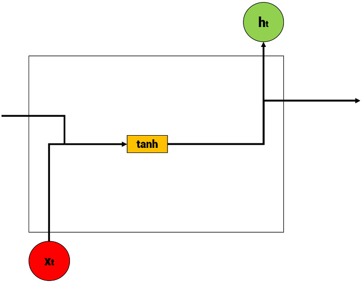
Illustration of recurrent neural network (RNN)
Recurrent neural network (RNN)
RNN is an artificial neural network in which directed connections connect hidden nodes to form a recurrent structure. It is a model suitable for sequential data processing, such as voice and text. In particular, it is mainly used in prediction problems using time series data in the financial field. Since RNN is a network structure that can accept input and output regardless of sequence length, the most significant advantage is that it can make structures diverse and flexible depending on the experimenter’s needs.
Long short-term memory (LSTM)
LSTM is a machine learning model that complements the traditional RNN’s vanishing gradient problem. LSTM adds input gates, forgetting gates, and output gates to memory cells of RNN in the hidden layer to erase unnecessary previous results and determine the results to be maintained. In addition, LSTM is a model in which the equation for calculating hidden states has become a little more complex than vanilla RNNs, and a new value of cell states has been added. As a result, LSTM usually performs better in processing sequential order input forms than RNNs (Fig. 5).
Fig. 5.

Illustration of long short-term memory (LSTM)
Gated recurrent unit (GRU)
GRU is a model that reduces calculations that update hidden status while maintaining LSTM’s complementary points of RNN’s vanishing gradient problem. In particular, in the LSTM, there are three gates: output, input, and delete gates, whereas in the GRU, there are only two gates, an update gate, and a reset gate, so the parameters are less than those of the LSTM (Fig. 6).
Fig. 6.
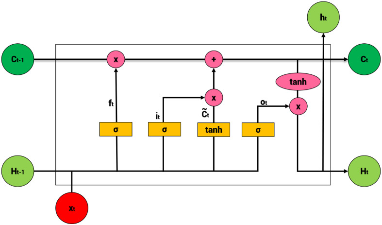
Illustration of gated recurrent unit (GRU)
Performance metrics of machine learning models
Nine machine learning models for forecasting the rise or fall of the currency values are evaluated by two evaluation metrics: accuracy and macro F1 score. Also, the value forecasting performance of the four machine learning models is evaluated by three common evaluation metrics: root mean squared error (RMSE), mean absolute error (MAE), and median absolute error (MDAE) for robustness. These evaluation metrics were selected based on the following prior research of forecasting financial indices or prices: RMSE (He & Droppo, 2016, Ni et al., 2019), MAE (Chen etal., 2018, Zeng & Khushi, 2020), and MDAE (Rounaghi & Zadeh, 2016, Berkman et al., 2000). The illustration of the confusion matrix and the calculation of each metric are as follows (Fig. 7):
| 13 |
| 14 |
| 15 |
| 16 |
| 17 |
Fig. 7.

Illustration of a confusion matrix
Calculation and analysis results
This section aimed to derive two features that would enhance the machine learning models’ ability to predict fluctuations of currency values based on information theory and network analysis. First, we determined the centrality degree of currencies with PageRank values based on the ETE value that implies the causality between currencies. Second, we grouped similar currencies into communities with hierarchical clustering.
ETE calculation results
We can measure the amount of reduction in information uncertainty, which means one currency has on another, and quantify the nonlinear causal relationship through ETE. With four datasets, among the total possible connections, this study used statistically significant transfer entropy values under significance levels for the stability of the results. The number of significant causal connections under the significance level = 0.1, 0.05, and 0.01 for the four datasets are shown in Table 5. The value in parentheses refers to the percentage of the actual number of connection nodes compared to the total number of possible nodes and the network’s density.
Table 5.
Number of significant ETE connections of each network by significance level
| Currency price change rate | 5d EVaR | 10d EVaR | 20d EVaR | |
|---|---|---|---|---|
| 524(23.22%) | 1033(45.79%) | 1013(44.90%) | 1018(45.12%) | |
| 496(21.99%) | 729(32.31%) | 718(31.83%) | 714(31.65%) | |
| 431(19.0%) | 276(12.23%) | 295(13.08%) | 289(12.81%) |
Network analysis result
With the calculated ETE values, this study illustrated a directed weighted network among the currencies with the start node as a source, the end node as a target, and ETE values as weights, as we mentioned before.
Network illustration
Figures 8, 9, 10, 11 displays the log-return, 5-day EVaR, 10-day EVaR, and 20-day EVaR networks of the total currencies. Each node is placed on the analyzed countries, thus representing the currencies. The width of the edges was multiplied by the transfer entropy values, thus representing the degree of correlation, i.e., the thicker edge means the higher correlation.
Fig. 8.

Network representation of log-returns
Fig. 9.

Network representation of 5-day EVaR
Fig. 10.

Network representation of 10-day EVaR
Fig. 11.

Network representation of 20-day EVaR
Comparing the edge thicknesses between the figures shows that the values of the ETE of EVaRs are relatively smaller than the value of the log-returns. In addition, the connection of the log-returns of gold price per ounce in the currency network plot is relatively sparse than that of the three rates of change of EVaR plots, indicating that fewer countries are in a causal relationship. What is noticeable is that the causal relationship of the US dollar, currently used as the significant key currency, is very low for every network. The number of connections in the US dollar is less than two, and the thickness of connections is also very lean, which is significantly different from other countries.
PageRank analysis
To analyze the most influential currency, we used PageRank to determine the centrality of each currency. The PageRank value was calculated by substituting the networks into the PageRank algorithm. The results indicate that the higher the PageRank value, the higher the centrality of the currency. Based on these calculation results, we visualized the network again to emphasize the centrality and classify currencies that act as key currencies.
Figures 12, 13, 14, 15 visualizes the networks with centrality taken into consideration. The size and color of each node were set to reflect the corresponding PageRank values. In the figures, the bluer to yellow the node becomes, and the larger the node becomes, the stronger the centrality. The noteworthy aspect of the analysis result is that the top three central countries were constant among EVaR networks. The first to third place was fixed as JPY, IDR, and KRW each. Thus, it could be seen that the currency values’ downside risks are forming a nonlinear causal network centered on JPY, IDR, and KRW. The log-return figure shows that KRW and IDR had the highest PageRank, while other countries had similar figures. This result implies that KRW and IDR act as a core in the global market fluctuation flow from the perspective of downside risks.
Fig. 12.

Network representation of log-returns based on PageRank
Fig. 13.

Network representation of 5-day EVaR based on PageRank
Fig. 14.

Network representation of 10-day EVaR based on PageRank
Fig. 15.

Network representation of 20-day EVaR based on PageRank
The key currencies and their corresponding PageRank values of each network are given in Table 6. Based on the PageRank values, we extracted key currencies from each network. The criterion for key currencies was set as the point at which the PageRank value began to converge. This point can be examined in Fig. 16, 17, 18, 19, which illustrates the PageRank values of each network in descending order.
Table 6.
Key currencies of each network based on PageRank
| Logarithmic returns | 5-day EVaR | 10-day EVaR | 20-day EVaR | ||||
|---|---|---|---|---|---|---|---|
| Currency | Centrality | Currency | Centrality | Currency | Centrality | Currency | Centrality |
| KRW | 0.2259 | JPY | 0.2263 | JPY | 0.1577 | JPY | 0.1669 |
| IDR | 0.1124 | IDR | 0.1240 | IDR | 0.1256 | IDR | 0.1202 |
| ISK | 0.0759 | KRW | 0.0934 | KRW | 0.0979 | KRW | 0.0915 |
| EGP | 0.0691 | PHP | 0.0673 | EGP | 0.0761 | ||
| RUB | 0.0442 | ||||||
Fig. 16.

PageRank values of log-return network
Fig. 17.

PageRank values of 5-day EVaR network
Fig. 18.

PageRank values of 10-day EVaR network
Fig. 19.

PageRank values of 20-day EVaR netw
Hierarchical clustering
Hierarchical clustering allows for determining the optimal cluster without predetermining the number of communities. We did not predetermine the particular degree of communities, making this method applicable flexibly. The feature in identifying the cluster is the distance of the currency network derived in Sect. 3.2.3. The distance between nodes was calculated into a distance matrix using the Dijkstra algorithm, commonly used to obtain the shortest distance of a weighted network. Then, the hierarchical clustering was performed using this distance matrix. This result grouped the log-returns, 5-day EVaR, 10-day EVaR, and 20-day EVaR into 10, 10, 14, and 15 communities, respectively. The communities within each network are presented in Tables 7, 8, 9, 10.
Table 7.
Communities of the log-return network
| Currencies | |||||||
|---|---|---|---|---|---|---|---|
| Cluster 1 | ATS | RUB | CHF | AED | THB | MXN | |
| Cluster 2 | CNY | DEM | GRD | ILS | ZAR | ESP | SEK |
| Cluster 3 | CLP | DKK | NLG | EUR | FIM | FRF | HKD |
| INR | IEP | ITL | MYR | PHP | PTE | LKR | |
| VND | |||||||
| Cluster 4 | ISK | TRY | KRW | GBP | HUF | JPY | SAR |
| Cluster 5 | EGP | BRL | PLN | ||||
| Cluster 6 | USD | AUD | IDR | NOK | CAD | ||
| Cluster 7 | BEF | NZD | |||||
| Cluster 8 | KWD | ||||||
| Cluster 9 | SGD | ||||||
| Cluster 10 | TWD | ||||||
Table 8.
Communities of the 5-day EVaR network
| Currencies | |||||||
|---|---|---|---|---|---|---|---|
| Cluster 1 | HKD | LKR | USD | ||||
| Cluster 2 | AUD | EGP | THB | BEF | HUF | FIM | IEP |
| Cluster 3 | SGD | ZAR | INR | MXN | SAR | EUR | ISK |
| Cluster 4 | JPY | TWD | IDR | KRW | CLP | CHF | DKK |
| Cluster 5 | NZD | CAD | NLG | GRD | |||
| Cluster 6 | GBP | RUB | VND | ITL | |||
| Cluster 7 | ATS | BRL | FRF | ||||
| Cluster 8 | AED | ILS | NOK | SEK | |||
| Cluster 9 | TRY | PHP | CNY | MYR | PTE | ||
| Cluster 10 | KWD | DEM | ESP | PLN | |||
Table 9.
Communities of the 10-day EVaR network
| Currencies | |||||||
|---|---|---|---|---|---|---|---|
| Cluster 1 | AUD | EGP | CNY | HKD | SLR | USD | |
| Cluster 2 | SAR | THB | NOK | ||||
| Cluster 3 | TRY | KRW | CAD | EUR | |||
| Cluster 4 | INR | CLP | PTE | ||||
| Cluster 5 | IDR | GRD | |||||
| Cluster 6 | TWD | CHF | |||||
| Cluster 7 | ATS | BEF | DKK | ||||
| Cluster 8 | BRL | FIM | |||||
| Cluster 9 | ZAR | KWD | HUF | VND | |||
| Cluster 10 | SGD | PHP | ILS | IEP | |||
| Cluster 11 | JPY | RUB | MXN | AED | NLG | LSK | |
| Cluster 12 | FRF | ||||||
| Cluster 13 | NZD | GBP | PLN | DEM | ITL | ESP | SEK |
| Cluster 14 | MYR | ||||||
Table 10.
Communities of the 20-day EVaR network
| Currencies | |||||||
|---|---|---|---|---|---|---|---|
| Cluster 1 | AUD | EGP | USD | HKD | ZAR | FIM | ITL |
| Cluster 2 | JPY | SAR | NLG | ||||
| Cluster 3 | MYR | BEF | CAD | GRD | |||
| Cluster 4 | SGD | PHP | DKK | ||||
| Cluster 5 | TYR | NZD | ISK | ||||
| Cluster 6 | THB | KRW | CLP | CHF | |||
| Cluster 7 | BRL | ||||||
| Cluster 8 | INR | RUB | LKR | IEP | |||
| Cluster 9 | TWD | FRF | |||||
| Cluster 10 | ATS | GBP | CNY | VND | |||
| Cluster 11 | KWD | HUF | |||||
| Cluster 12 | MXN | AED | EUR | ||||
| Cluster 13 | PTE | ESP | NOK | PLN | SEK | ||
| Cluster 14 | IDR | DEM | |||||
| Cluster 15 | ILS | ||||||
Prediction based on network analysis results
Prediction experiment layouts
Using the results in Sect. 4, we predicted the fluctuations and log-returns of gold price per ounce in currencies. As we mentioned above, we predicted the currency price of gold per troy ounce using four(log-return, 5-day EVaR, 10-day EVaR, and 20-day EVaR) constructed networks.
According to prior research, price prediction is mainly addressed in two types of problems: classification and regression. Thus, we considered both classification and regression problems to take into account the robustness of our experimental results.
In constructing these experiments, we referred to other prior research that planned experiments similar to this study and suggested improvements in the existing models and evaluation performances (Jana, 2021a; Liu et al., 2019; Jana, 2021b; Jana & Ghosh, 2018; Jana & Pal, 2021; Jana et al., 2021). These studies effectively improved decision-making and prediction models, which are similar to the proposed models in this study.
To check the prediction results based on our network, we performed four experiments by differing the use of results in Sect. 4. Experiment 1 was used as a baseline experiment by using the log-returns and EVaR of gold price per ounce in currencies data of the entire 48 countries in prediction. The other three experiments were designed to check the influence using the information flow network-based clustering results and PageRank-based key currency results. Experiment 2 used network-based clustering results, which means it used only the data columns in the same communities. Experiment 3 used the PageRank-based key currency results, and experiment 4 used both clustering and PageRank-based key currency results.
Clustering results refer to the result in Sect. 4.2.3, where similar currencies were grouped into communities based on the network distance. Experiment 2 used other currency data from the same community to predict currency prices. Centrality result refers to the outcomes from Sect. 4.2.2, where key currencies were chosen based on the PageRank of the network. Experiment 3 included the currency price data from the key currencies in predicting the currency price of one country, and Experiment 4 contained both clustering and centrality data in the prediction. Finally, we conducted prediction experiments of the fluctuations and log-return values, including 5-day EVaR, 10-day EVaR, and 20-day EVaR values, also using their centrality measures as we mentioned above.
Two sub-experiments were performed for each experiment: predicting the fluctuation and the value. Every experiment was performed on the four datasets, meaning 32 experiment iterations. For the stability of this study, each experiment iteration was conducted with 500 times simulations (5 optimization algorithms, 20 iterations, 5 cross-validations) with 1000 times learning iterations. We experimented using five optimizers, which are methods of finding optimal weights through machine learning. First, we selected the most widely used algorithms in recent studies: Stochastic Gradient Descent (SGD), AdaGrad, RMSProp, Adam, and AdaDelta. Then, we selected the best model from the experiments using different optimizers. The metrics for evaluating the models were used differently for two sub-experiments: in predicting the fluctuation, accuracy and macro F1 score were used, and for predicting the value, we used MAE, RMSE, and MDAE. The machine learning models for each sub-experiment are explained in Sect. 3.3. The summarized description of the experiment can be found in Table 11.
Table 11.
Experiment description
| Category | Experiment 1 | Experiment 2 | Experiment 3 | Experiment 4 |
|---|---|---|---|---|
| Subjects | 48 countries | |||
| Dataset | Logarithmic returns, 5-day EVaR, 10-day EVaR, 20-day EVaR | |||
| Types | 1. Prediction of fluctuation | |||
| 2. Prediction of log price rates of change | ||||
| Simulations | 500 times | |||
| Iterations | 1000 times | |||
| Metrics | 1. Accuracy, macro F1 score (for classification) | |||
| 2. MAE, RMSE, MDAE (for regresssion) | ||||
| Ex rate data | Yes | Yes | Yes | Yes |
| Clustering result | No | Yes | No | Yes |
| Centrality result | No | No | Yes | Yes |
Prediction result
The experiment results mentioned in Sect. 5.1 are as follows. First, the average value and the 95% confidence interval for predicting the currency price fluctuation are given in Tables 12, 13. Second, in prediction, a value of 1 was given if the currency price was rising or maintained and 0 if it was falling, making the experiment a case of classification. Third, comparing the metric values confirmed that the average accuracy and macro F1 scores in Experiments 2, 3, and 4 improved compared to Experiment 1 for every machine learning model. Moreover, statistically significant results were derived under the significance level , under the paired t-sample test on the accuracy and macro F1 score results. The result implies that Experiment 2, Experiment 3, and Experiment 4 showed statistically better prediction results for predicting rise and fall of the currency values on the following day compared to Experiment 1.
Table 12.
Accuracy in predicting the change in log-returns of gold price per ounce in currencies (%)
| ML Model | Experiment 1 | Experiment 2 | Experiment 3 | Experiment 4 |
|---|---|---|---|---|
| LR | ||||
| DT | ||||
| KM | ||||
| XGB | ||||
| LBM | ||||
| SVM | ||||
| RF | ||||
| GNB | ||||
| MLP |
Table 13.
Macro F1 scores in predicting the change in log-returns of gold price per ounce in currencies (%)
| ML Model | Experiment 1 | Experiment 2 | Experiment 3 | Experiment 4 |
|---|---|---|---|---|
| LR | ||||
| DT | ||||
| KM | ||||
| XGB | ||||
| LBM | ||||
| SVM | ||||
| RF | ||||
| GNB | ||||
| MLP |
Second, the average result value and the 95% confidence interval in the case of predicting the log-returns are given in Tables 14, 15, 16. Although all log-return forecasts do not indicate a strong statement as in the classification problem, deriving the number of currencies that showed improved metric scores showed meaningful results. In Experiment 2, it was confirmed that approximately 70% or more (34–36) of data displayed improved metric scores. Furthermore, by comparing the number of improved countries, Experiment 3 showed slightly better results than Experiment 2. Experiment 4, which combined the clustering and centrality results, showed the most improved prediction results: Over 80% improved currencies compared to Experiment 1. From Table 14, there were cases where the average MAE, RMSE, and MDAE values increased while the number of improved results increased. Such results could be understood as an outlier due to tremendous error values in some countries. Also, those currencies with very few constituents in their communities in EVaR got relatively worse results.
Table 14.
Average MAE scores in predicting log-returns of gold price per ounce in currencies (%)
| ML Model | Experiment 1 | Experiment 2 | Experiment 3 | Experiment 4 |
|---|---|---|---|---|
| CNN | 3.55 | 4.20 | 3.49 | 2.44 |
| RNN | 3.57 | 4.13 | 3.49 | 3.53 |
| LSTM | 3.56 | 4.12 | 3.48 | 3.51 |
| GRU | 3.57 | 4.12 | 3.48 | 3.51 |
The first value in the parentheses refers to the number of improved currencies compared to the first experiment, and the second value refers to the improvement in percentage
Table 15.
Average MSE scores in predicting log-returns of gold price per ounce in currencies (%)
| ML Model | Experiment 1 | Experiment 2 | Experiment 3 | Experiment 4 |
|---|---|---|---|---|
| CNN | 5.05 | 5.73 | 5.08 | 5.09 |
| RNN | 4.98 | 5.65 | 5.00 | 4.89 |
| LSTM | 4.99 | 5.64 | 5.01 | 4.88 |
| GRU | 4.98 | 5.64 | 5.01 | 4.89 |
The first value in the parentheses refers to the number of improved currencies compared to the first experiment, and the second value refers to the improvement in percentage
Table 16.
Average MDAE scores in predicting log-returns of gold price per ounce in currencies (%)
| ML Model | Experiment 1 | Experiment 2 | Experiment 3 | Experiment 4 |
|---|---|---|---|---|
| CNN | 3.04 | 3.53 | 2.93 | 3.09 |
| RNN | 2.97 | 3.51 | 3.03 | 3.01 |
| LSTM | 2.96 | 3.51 | 2.98 | 2.99 |
| GRU | 2.96 | 3.50 | 2.99 | 2.99 |
The first value in the parentheses refers to the number of improved currencies compared to the first experiment, and the second value refers to the improvement in percentage
In sum, the results of this study can be translated as that predictive power can be improved like the results of prior research as mentioned at the top of Sect. 5.1. This result means that methods using network characteristics can improve predictive power through more efficient data utilization.
Conclusion
This study aimed to improve the exchange rates prediction performance using the causal relationships between log-returns and downside risks of currency values derived from gold and modeling them as networks. We have calculated the causal relationship of log-return, 5-day EVaR, 10-day EVaR, and 20-day EVaR values of currency values through effective transfer entropy. Based on the constructed networks, we generated communities based on their network topology and used them to improve the machine learning-based prediction performance of fluctuations in currency values.
As a result of visualizing the directed weighted networks with the transfer entropy as weights, we discovered the novel relationships based on log-return and downside risk values of currency values. For example, the primary currency based on global economic power and the major currency based on causality networks’ centrality measures differed. Using the clustering results derived from the topology of constructed networks for machine learning, we found that the performance statistically significantly improved despite decreasing the number of data columns. Thus, these results can help predict exchange rates in a roundabout way.
This study attempted to present a novel methodology for predicting exchange rates and analyzing exchange rates via log-returns and downside risks of gold price per ounce in currencies. However, factors affecting macroeconomic variables are vast and highly uncertain, making them difficult to quantify. Moreover, quantifying factors based only on currency-related variables may result in a bias, resulting in poor prediction performance as in Experiment 1 of Sect. 5.
However, this study’s novel contribution can be summarized as follows:
We illustrated causal relationships based on log-returns and downside risks of gold price per ounce in currencies calculated by effective transfer entropy and analyzed through network theory.
Based on the illustrated log-return and downside risk networks, We used them to reduce information uncertainty in exchange rate prediction, resulting in better or almost similar results even though fewer data were used.
Since resolving information uncertainty is a significant factor in prediction, the results of this study can be expected to provide a different view on forecasting exchange rate prediction from the perspective of computation efficiency and feature selection.
It would be possible to apply more advanced machine learning algorithms for further studies. The models we used were basic machine learning algorithms utilized widely but not conducted based on the latest machine learning model. In addition, the relationship network we constructed only considered causal relationships between currencies and did not encompass other macroeconomic variables that would affect the exchange rates. The following research could derive more quantitatively developed results considering those improvements. Finally, it would be possible to combine the results with reinforcement learning-based foreign exchange investment methodology and expand in predicting the future price rates of change and risk fluctuations.
Acknowledgements
The authors sincerely appreciate the editors and anonymous reviewers for their feedback and suggestions for improving this study.
Availability of data and materials
The datasets generated or analyzed during the current study are available in the pacific exchange rates service repository, http://fx.sauder.ubc.ca/data.html. The datasets generated or analyzed during the current study are available in the World Gold Council repository, https://www.gold.org/goldhub/data/gold-prices. The datasets generated or analyzed during the current study are available in the Korea Economic Statistics System repository, https://ecos.bok.or.kr/. The datasets generated or analyzed during the current study are available in the Chile Banco Central repository, https://si3.bcentral.cl/Siete/ES/Siete/Cuadro/CAP_TIPO_CAMBIO/MN_TIPO_CAMBIO4/DOLAR_OBS_ADO/TCB_505. The datasets generated or analyzed during the current study are available in the Central Bank of Kuwait repository, https://www.cbk.gov.kw/en/monetary-policy/market-operations/exchange-rates. The datasets generated or analyzed during the current study are available in the Board of Governors of the Federal Reserve System repository, https://www.federalreserve.gov/releases/h10/hist/dat96_bz.htm. The datasets generated or analyzed during the current study are available in the Central Bank of Sri Lanka repository, https://www.cbsl.gov.lk/en/rates-and-indicators/exchange-rates.
Declarations
Conflict of interest
The authors have no relevant financial or non-financial interests to disclose.
Footnotes
Publisher's Note
Springer Nature remains neutral with regard to jurisdictional claims in published maps and institutional affiliations.
Contributor Information
Insu Choi, Email: jl.cheivly@kaist.ac.kr.
Wonje Yun, Email: wjy1993@kaist.ac.kr.
Woo Chang Kim, Email: wkim@kaist.ac.kr.
References
- Abbasi, R. A., Javaid, N., Ghuman, M. N. J., Khan, Z. A., Ur Rehman, S., & Amanullah. (2019). Short term load forecasting using xgboost. L. Barolli, M. Takizawa, F. Xhafa, & T. Enokido (Eds.), Web, artificial intelligence and network applications (pp. 1120–1131). Cham: Springer International Publishing.
- Ahmadi-Javid A. Entropic value-at-risk: A new coherent risk measure. Journal of Optimization Theory and Applications. 2012;155(3):1105–1123. doi: 10.1007/s10957-011-9968-2. [DOI] [Google Scholar]
- Antweiler, W. (2008). Pacific exchange rate service-database retrieval system. Available at http://fx.sauder.ubc.ca/data.html.
- Bekiros S, Nguyen DK, Junior LS, Uddin GS. Information diffusion, cluster formation and entropy-based network dynamics in equity and commodity markets. European Journal of Operational Research. 2017;256(3):945–961. doi: 10.1016/j.ejor.2016.06.052. [DOI] [Google Scholar]
- Belhadi, A., Kamble, S. S., Mani, V., Benkhati, I., & Touriki, F. E. (2021). An ensemble machine learning approach for forecasting credit risk of agricultural SMEs’ investments in agriculture 4.0 through supply chain finance. Annals of Operations Research, 1–29. [DOI] [PMC free article] [PubMed]
- Berkman H, Bradbury ME, Ferguson J. The accuracy of priceearnings and discounted cash flow methods of IPO equity valuation. Journal of International Financial Management & Accounting. 2000;11(2):71–83. doi: 10.1111/1467-646X.00056. [DOI] [Google Scholar]
- Board of Governors of the Federal Reserve System (2021). H.10 brazil historical rates. Available at https://www.federalreserve.gov/releases/h10/hist/dat96 bz.htm (1999/12/31).
- Boba P, Bollmann D, Schoepe D, Wester N, Wiesel J, Hamacher K. Efficient computation and statistical assessment of transfer entropy. Frontiers in Physics. 2015;3:10. doi: 10.3389/fphy.2015.00010. [DOI] [Google Scholar]
- Boehmke, B., & Greenwell, B. (2019). Hands-on machine learning with R. Chapman and Hall/CRC.
- Bohdalová, M. (2007). A comparison of value-at-risk methods for measurement of the financial risk (p. 10). Faculty of Management: Comenius University, Bratislava, Slovakia.
- Cao G, Zhang Q, Li Q. Causal relationship between the global foreign exchange market based on complex networks and entropy theory. Chaos, Solitons & Fractals. 2017;99:36–44. doi: 10.1016/j.chaos.2017.03.039. [DOI] [Google Scholar]
- Central Bank of Kuwait (2021). Foreign currencies exchange rates. Available at https://www.cbk.gov.kw/en/monetary-policy/market-operations/exchange-rates.
- Central Bank of Sri Lanka (2021). Exchange rates: Central bank of Sri Lanka. Available at https://www.cbsl.gov.lk/en/rates-and-indicators/exchange-rates.
- Chen, T., & Guestrin, C. (2016). Xgboost: A scalable tree boosting system. In Proceedings of the 22nd ACM SIGKDD international conference on knowledge discovery and data mining (pp. 785–794).
- Chen W, Yeo CK, Lau CT, Lee BS. Leveraging social media news to predict stock index movement using RNN-boost. Data & Knowledge Engineering. 2018;118:14–24. doi: 10.1016/j.datak.2018.08.003. [DOI] [Google Scholar]
- Chile Banco Central (2021). Exchange rates-observed dollar. Available at https://si3.bcentral.cl/Siete/ES/Siete/Cuadro/CAP_TIPO_CAMBIO/MN TIPO_CAMBIO4/DOLAR_OBS_ADO/TCB_505.
- Choi I, Kim WC. Detecting and analyzing politically-themed stocks using text mining techniques and transfer entropy|focus on the republic of korea’s case. Entropy. 2021;23(6):734. doi: 10.3390/e23060734. [DOI] [PMC free article] [PubMed] [Google Scholar]
- Cristianini N, Shawe-Taylor J, et al. An introduction to support vector machines and other kernel-based learning methods. Cambridge: Cambridge University Press; 2000. [Google Scholar]
- Dimpfl, T., & Peter, F. J. (2013). Using transfer entropy to measure information flows between financial markets. Studies in Nonlinear Dynamics and Econometrics, 17(1), 85–102.
- Friedman, J. H. (2001). Greedy function approximation: A gradient boosting machine. Annals of Statistics, 1189–1232.
- Galeshchuk S. Neural networks performance in exchange rate prediction. Neurocomputing. 2016;172:446–452. doi: 10.1016/j.neucom.2015.03.100. [DOI] [Google Scholar]
- Granger, C. W. (1969). Investigating causal relations by econometric models and cross-spectral methods. Econometrica: Journal of the Econometric Society, 424–438.
- Gumus, M., & Kiran, M. S. (2017). Crude oil price forecasting using xgboost. In 2017 international conference on computer science and engineering (UBMK) (pp. 1100–1103).
- Gupta S, Modgil S, Bhattacharyya S, Bose I. Artificial intelligence for decision support systems in the field of operations research: Review and future scope of research. Annals of Operations Research. 2022;308:215–274. doi: 10.1007/s10479-020-03856-6. [DOI] [Google Scholar]
- Hacine-Gharbi A, Ravier P. A binning formula of bi-histogram for joint entropy estimation using mean square error minimization. Pattern Recognition Letters. 2018;101:21–28. doi: 10.1016/j.patrec.2017.11.007. [DOI] [Google Scholar]
- Hacine-Gharbi A, Ravier P, Harba R, Mohamadi T. Low bias histogram-based estimation of mutual information for feature selection. Pattern Recognition Letters. 2012;33(10):1302–1308. doi: 10.1016/j.patrec.2012.02.022. [DOI] [Google Scholar]
- Hastie, T., Tibshirani, R., Friedman, J. H., & Friedman, J. H. (2009). The elements of statistical learning: Data mining, inference, and prediction (Vol. 2). Springer.
- He, T., & Droppo, J. (2016). Exploiting LSTM structure in deep neural networks for speech recognition. In 2016 IEEE international conference on acoustics, speech and signal processing (ICASSP) (pp. 5445–5449).
- Jabeur, S. B., Mefteh-Wali, S., & Viviani, J.-L. (2021). Forecasting gold price with the xgboost algorithm and shap interaction values. Annals of Operations Research, 1–21.
- Jana C. Multiple attribute group decision-making method based on extended bipolar fuzzy mabac approach. Computational and Applied Mathematics. 2021;40(6):1–17. doi: 10.1007/s40314-021-01606-3. [DOI] [Google Scholar]
- Jana C. Multiple attribute group decision-making method based on extended bipolar fuzzy mabac approach. Computational and Applied Mathematics. 2021;40(6):1–17. doi: 10.1007/s40314-021-01606-3. [DOI] [Google Scholar]
- Jana C, Muhiuddin G, Pal M. Multi-criteria decision making approach based on svtrn dombi aggregation functions. Artificial Intelligence Review. 2021;54(5):3685–3723. doi: 10.1007/s10462-020-09936-0. [DOI] [Google Scholar]
- Jana C, Pal M. A dynamical hybrid method to design decision making process based on GRA approach for multiple attributes problem. Engineering Applications of Artificial Intelligence. 2021;100:104203. doi: 10.1016/j.engappai.2021.104203. [DOI] [Google Scholar]
- Jana DK, Bhunia P, Adhikary SD, Bej B. Optimization of effluents using artificial neural network and support vector regression in detergent industrial wastewater treatment. Cleaner Chemical Engineering. 2022;3:100039. doi: 10.1016/j.clce.2022.100039. [DOI] [Google Scholar]
- Jana DK, Ghosh R. Novel interval type-2 fuzzy logic controller for improving risk assessment model of cyber security. Journal of Information Security and Applications. 2018;40:173–182. doi: 10.1016/j.jisa.2018.04.002. [DOI] [Google Scholar]
- Jang SM, Yi E, Kim WC, Ahn K. Information flow between bitcoin and other investment assets. Entropy. 2019;21(11):1116. doi: 10.3390/e21111116. [DOI] [Google Scholar]
- Ke G, Meng Q, Finley T, Wang T, Chen W, Ma W, Liu T-Y. Lightgbm: A highly efficient gradient boosting decision tree. Advances in Neural Information Processing Systems. 2017;30:3146–3154. [Google Scholar]
- Knuth KH. Optimal data-based binning for histograms and histogram-based probability density models. Digital Signal Processing. 2019;95:102581. doi: 10.1016/j.dsp.2019.102581. [DOI] [Google Scholar]
- Korea Economic Statistics System (2021). The US dollar exchange rate of major currencies. Available at https://ecos.bok.or.kr/.
- Kwak K-Y. Social network analysis. Seoul: ChungRam; 2017. [Google Scholar]
- Kwon O, Yang J-S. Information flow between composite stock index and individual stocks. Physica A: Statistical Mechanics and its Applications. 2008;387(12):2851–2856. doi: 10.1016/j.physa.2008.01.007. [DOI] [Google Scholar]
- Lee S. Network analysis methodology. Seoul: NonHyung; 2013. [Google Scholar]
- Li, S. Z. (2009). Encyclopedia of biometrics: I-z. (Vol. 2). Springer Science & Business Media.
- Lim K, Kim S, Kim SY. Information transfer across intra/interstructure of CDS and stock markets. Physica A: Statistical Mechanics and its Applications. 2017;486:118–126. doi: 10.1016/j.physa.2017.05.084. [DOI] [Google Scholar]
- Lisi F, Schiavo RA. A comparison between neural networks and chaotic models for exchange rate prediction. Computational Statistics & Data Analysis. 1999;30(1):87–102. doi: 10.1016/S0167-9473(98)00067-X. [DOI] [Google Scholar]
- Liu J, Wu C, Li Y. Improving financial distress prediction using financial network-based information and GA-based gradient boosting method. Computational Economics. 2019;53(2):851–872. doi: 10.1007/s10614-017-9768-3. [DOI] [Google Scholar]
- Liu, L., Ye, Y.-t., Xie, Y., & Pu, L. (2010). Serial number extracting and recognizing applied in paper currency sorting system based on RBF network. In 2010 international conference on computational intelligence and software engineering (pp. 1–4).
- Marschinski R, Kantz H. Analysing the information flow between financial time series. The European Physical Journal B-Condensed Matter and Complex Systems. 2002;30(2):275–281. doi: 10.1140/epjb/e2002-00379-2. [DOI] [Google Scholar]
- Mo B, Nie H, Jiang Y. Dynamic linkages among the gold market, us dollar and crude oil market. Physica A: Statistical Mechanics and its Applications. 2018;491:984–994. doi: 10.1016/j.physa.2017.09.091. [DOI] [Google Scholar]
- Molnar, C. (2018). A guide for making black box models explainable. Available at https://christophm.github.io/interpretable-ml-book.
- Ni L, Li Y, Wang X, Zhang J, Yu J, Qi C. Forecasting of forex time series data based on deep learning. Procedia Computer Science. 2019;147:647–652. doi: 10.1016/j.procs.2019.01.189. [DOI] [Google Scholar]
- Page, L., Brin, S., Motwani, R., & Winograd, T. (1999). The pagerank citation ranking: Bringing order to the web. (Technical Report). Stanford InfoLab.
- Pedregosa F, Varoquaux G, Gramfort A, Michel V, Thirion B, Grisel O, Duchesnay E. Scikit-learn: Machine learning in Python. Journal of Machine Learning Research. 2011;12:2825–2830. [Google Scholar]
- Platt J, et al. Probabilistic outputs for support vector machines and comparisons to regularized likelihood methods. Advances in Large Margin Classifiers. 1999;10(3):61–74. [Google Scholar]
- Rounaghi MM, Zadeh FN. Investigation of market efficiency and financial stability between s &p 500 and London stock exchange: Monthly and yearly forecasting of time series stock returns using arma model. Physica A: Statistical Mechanics and its Applications. 2016;456:10–21. doi: 10.1016/j.physa.2016.03.006. [DOI] [Google Scholar]
- Sayavong, L., Wu, Z., & Chalita, S. (2019). Research on stock price prediction method based on convolutional neural network. In 2019 international conference on virtual reality and intelligent systems (ICVRIS) (pp. 173–176).
- Schreiber T. Measuring information transfer. Physical Review Letters. 2000;85(2):461. doi: 10.1103/PhysRevLett.85.461. [DOI] [PubMed] [Google Scholar]
- Sensoy A, Sobaci C, Sensoy S, Alali F. Effective transfer entropy approach to information flow between exchange rates and stock markets. Chaos, Solitons & Fractals. 2014;68:180–185. doi: 10.1016/j.chaos.2014.08.007. [DOI] [Google Scholar]
- Séverin E, Veganzones D. Can earnings management information improve bankruptcy prediction models? Annals of Operations Research. 2021;306(1):247–272. doi: 10.1007/s10479-021-04183-0. [DOI] [Google Scholar]
- Sheikh AZ, Qiao H. Non-normality of market returns: A framework for asset allocation decision making. The Journal of Alternative Investments. 2009;12(3):8–35. doi: 10.3905/JAI.2010.12.3.008. [DOI] [Google Scholar]
- Sun X, Liu M, Sima Z. A novel cryptocurrency price trend forecasting model based on lightgbm. Finance Research Letters. 2020;32:101084. doi: 10.1016/j.frl.2018.12.032. [DOI] [Google Scholar]
- Tsai, C.S.-Y. (2011). The real world is not normal. IL, USA: Morningstar Alternative Investments Observer:Chicago.
- World Gold Council (2021). Gold price historical data: Gold price history. Available at https://www.gold.org/goldhub/data/gold-prices (2021/09).
- Yue P, Cai Q, Yan W, Zhou W-X. Information flow networks of Chinese stock market sectors. IEEE Access. 2020;8:13066–13077. doi: 10.1109/ACCESS.2020.2966278. [DOI] [Google Scholar]
- Yue P, Fan Y, Batten JA, Zhou W-X. Information transfer between stock market sectors: A comparison between the USA and China. Entropy. 2020;22(2):194. doi: 10.3390/e22020194. [DOI] [PMC free article] [PubMed] [Google Scholar]
- Yun KK, Yoon SW, Won D. Prediction of stock price direction using a hybrid GA-xgboost algorithm with a three-stage feature engineering process. Expert Systems with Applications. 2021;186:115716. doi: 10.1016/j.eswa.2021.115716. [DOI] [Google Scholar]
- Zeng, Z., & Khushi, M. (2020). Wavelet denoising and attention-based rnnarima model to predict forex price. In 2020 international joint conference on neural networks (IJCNN) (pp. 1–7).
- Zhukov, M., & Popov, A. (2014). Bin number selection for equidistant mutual information estimaton. In 2014 IEEE 34th international scientific conference on electronics and nanotechnology (ELNANO) (pp. 259–263).
Associated Data
This section collects any data citations, data availability statements, or supplementary materials included in this article.
Data Availability Statement
The datasets generated or analyzed during the current study are available in the pacific exchange rates service repository, http://fx.sauder.ubc.ca/data.html. The datasets generated or analyzed during the current study are available in the World Gold Council repository, https://www.gold.org/goldhub/data/gold-prices. The datasets generated or analyzed during the current study are available in the Korea Economic Statistics System repository, https://ecos.bok.or.kr/. The datasets generated or analyzed during the current study are available in the Chile Banco Central repository, https://si3.bcentral.cl/Siete/ES/Siete/Cuadro/CAP_TIPO_CAMBIO/MN_TIPO_CAMBIO4/DOLAR_OBS_ADO/TCB_505. The datasets generated or analyzed during the current study are available in the Central Bank of Kuwait repository, https://www.cbk.gov.kw/en/monetary-policy/market-operations/exchange-rates. The datasets generated or analyzed during the current study are available in the Board of Governors of the Federal Reserve System repository, https://www.federalreserve.gov/releases/h10/hist/dat96_bz.htm. The datasets generated or analyzed during the current study are available in the Central Bank of Sri Lanka repository, https://www.cbsl.gov.lk/en/rates-and-indicators/exchange-rates.