Development of a long-term time-weighted exposure metric that accounts for missing data in the Seychelles Child Development Study

Abstract

In many studies of the health effects of toxicants, exposure is measured once even though exposure may be continuous. However, some studies collect repeated measurements on participants over an extended time with the goal of determining a long-term metric that captures the average or cumulative exposure. This can be challenging, especially when exposure is measured at irregular intervals and has some missing values. Here we describe a method for determining a measure of long-term exposure using data on postnatal mercury (Hg) from the Seychelles Child Development Study (SCDS) Main Cohort as a model. In this cohort (n = 779), we incorporate postnatal Hg values that were measured on most study participants at seven ages, three between 6 months and 5.5 years (“childhood”), and an additional four between 17 and 24 years (“early adulthood”). We develop time-weighted measures of average exposure during the childhood and the early adulthood periods and compare the strengths and weaknesses of our metric to two standard measures: overall average and cumulative exposure. We account for missing values through an imputation method that uses information about age- and sex-specific Hg means and the participant’s Hg values at similar ages to estimate subject-specific missing Hg values. We compare our method to the implicit imputation assumed by these two standard methods, and to Fully Conditional Specification (FCS), an alternative method of imputing missing data. To determine the accuracy of our imputation method we use data from participants with no missing Hg values in the relevant time window. The imputed values from our proposed method are substantially closer to the observed values on average than the average or cumulative exposure, while also performing slightly better than FCS. In conclusion, time-weighted long-term exposure appears to offer advantages over cumulative exposure in longitudinal studies with repeated measures where the follow-up period for a toxicant is similar for all participants. Additionally, our method to impute missing values maximizes the number of participants for whom the overall exposure metric can be calculated and should provide a more accurate long-term exposure metric than standard methods when exposure has missing values. Our method is applicable to any study of long-term toxicant effects when longitudinal exposure measurements are available but have missing values.

1. Introduction

1.1. Background

Exposure to low levels of clinically silent toxicants is common. It is not clear whether repeated exposure to low levels of such toxicants over a prolonged time is harmful. To address this question, several studies have measured the exposure of interest on study participants at multiple ages, from which a long-term measure of exposure is then developed and examined in relation to outcomes of interest. However, there are differences of opinion about the best way to summarize multiple exposure measures into a single long-term measure for the period of interest. In addition, often participants do not have an exposure measure at every time point for which exposure measurement is planned. Typically, these participants are either excluded or exposure metrics are created only from the observed values, neither of which may be optimal. To address these issues, we develop a metric of long-term exposure for use with repeated measures of toxicant exposure, or more generally to any repeated biometric measurements, that can be applied when some of the measurements are missing.

Cumulative exposure is defined as the area under the curve (AUC) of exposure intensity over a specific time window and is a widely used measure that combines information about intensity and duration into a single metric. Whether cumulative exposure is useful for a particular situation depends on the disease process (Kriebel et al., 2007), which is not always well understood. Cumulative exposure is useful in some situations, such as for inhaled dust where it is proportional to the total dose in the lung assuming a constant ventilation rate (Kriebel et al, 2007). However, this metric does not allow investigators to estimate the relative impact of exposure intensity vs. exposure duration. One alternative is to evaluate associations with exposure intensity and duration as separate variables. When the window of exposure is similar for all participants, duration becomes less important than average intensity, and the latter is approximately proportional to cumulative exposure.

Other authors have proposed methods to examine the relationship between longitudinal exposure measures and a subsequent outcome. For example Chen et al. (2015) compared nine methods of examining longitudinal measures of phthalates during pregnancy in relation to preterm birth. One of the nine methods combined repeated exposures into a single metric using average exposure, while others model the relationship between exposure and time to obtain other exposure summaries. Chen et al. (2015) did not specifically address missing exposure measurements.

We take advantage of a large repository of exposure data in a long-standing prospective longitudinal cohort study to address the situation in which exposure is measured multiple times in approximately the same time window over several decades for all study participants. Our aim is to develop a summary exposure metric that best captures overall exposure during multi-year periods based on repeated exposure measurements that are irregularly spaced while also specifically accounting for missing values. These issues are often a challenge in multi-year studies of toxicant exposure.

1.2. Relation to prior work and overview of the paper

We develop longitudinal measures of Hg exposure using data from the Seychelles Child Development Study (SCDS) Main Cohort. We recruited the participants in 1989-1990 to study the association between mercury (Hg) exposure from fish consumption and the children’s neurodevelopmental outcomes measured at multiple ages. Most prior studies of this cohort have examined associations with prenatal Hg exposure measured in maternal hair grown during pregnancy. However, a recent focus of the SCDS is to understand associations between longitudinal measures of neurodevelopment and postnatal Hg exposure using information from multiple Hg measurements. The availability of postnatal Hg measurements at many time points makes the SCDS cohort a unique and suitable study to provide insights into how best to address the challenges inherent in creating long-term exposure measures. This work builds on our earlier publication (Myers et al., 2009), in which we developed three metrics of cumulative postnatal exposure using Hg measurements collected at three ages: 6, 19, and 66 months (5.5 years) of age. In that publication, we examined those metrics in relationship to 66 month and 9-year outcomes. Our high-low metric used Hg measures at 19 and 66 months, and categorized each participant into a “high” group (if both Hg measures were above a threshold, using several different thresholds) or a “low” group (if both Hg values were below a threshold). Our second metric was the area under the curve (AUC) of Hg exposure measured either from 19 to 66 months or from 6 to 66 months of age. Our third metric was similar to the AUC metric, but weighted the three Hg levels in proportion to the estimated rate of brain growth at that age. None of these metrics explicitly accounted for missing Hg. The largest number of missing Hg values occurred in the high-low metric because children who were in the “high” group at one age and the “low” group at the other age, or who were missing either Hg value, were excluded. Both AUC metrics required Hg measurements at the first and last age. Because many more participants were missing 6-month Hg than 19-month Hg, we based model results using these different Hg metrics on different subsets of participants. Consequently, a direct comparison of results was not possible.

To address concerns with use of the AUC metric when exposure data are missing, here we develop a new metric that addresses several complications inherent in creating a summary exposure metric based on multiple exposures measured over time. We address how to handle missing values of individual exposures and how to combine multiple exposure measurements to create a person-specific summary measure of exposure over the age range of interest. In Section 2.1 we discuss theoretical considerations of our methods for addressing missing exposure data and combining repeated exposure measures into a single metric. In Section 2.2 we give an overview of our approach and then describe our methods and evaluation criteria in relation to the SCDS. We present results of our method using SCDS data in Section 3, and finish with some discussion and conclusions in Sections 4 and 5.

2. Methods

2.1. Theoretical considerations

2.1.1. Missing exposure data

Missing exposure data for a subset of study participants is a frequent occurrence in longitudinal studies. Investigators take a variety of approaches to address this issue. A complete-case analysis, which drops observations that are missing exposure data at one or more time points, may be justifiable if the probability that an exposure value is missing (called the “missing data mechanism”) is unrelated to any aspect of the full data. In this situation, called “missing completely at random” dropping those observations would not bias the resulting estimates. However, if the missing data mechanism depends on other variables then dropping these observations can introduce bias (Rubin 1976, Little and Rubin 2019).

An alternative is to impute a value to replace each missing value. A number of ad-hoc strategies have been proposed to accomplish this including imputing the mean of the observed values of the variable, the subject’s previously observed value (if relevant) or a value from a different randomly chosen observation. These ad hoc strategies can lead to biased estimates (Schafer and Olsen 1998, Little and Rubin 2019). Alternatively, one could model the relationship between the variables in the model, and replace missing values with predicted values or with the predicted values plus random error. In predicting unmeasured data, knowledge about the missing data mechanism is also essential unless the data are missing completely at random. In particular, if the probability that data are missing can reasonably be assumed to depend on specific covariates, then using these covariates in the model to help estimate the missing value can reduce or eliminate bias (Little and Rubin, 2019). In the SCDS, the degree to which postnatal Hg data were missing depended on both the child’s sex (boys had shaved their heads at some visits, which precluded a Hg measurement), and different follow-up rates at the visit ages. Since the participants and examiners were blinded to previous exposure measurements, it is not likely that selective participation or collection of hair samples was related to exposure.

Imputing a single value for each missing exposure value ignores the uncertainty of the exposure measure (Little and Rubin, 2019). When used as a covariate in a regression model, using a single estimate of exposure will cause the standard error for the exposure slope to be underestimated. In multiple imputation, missing values are imputed multiple times to create K > 1 complete datasets. Inference is then based on fitting the model on each dataset and adjusting the variance of the slope appropriately to take into account the variability within and across the K datasets (Little and Rubin, 2019). Our ultimate goal is to create a single best longitudinal exposure summary metric for a given multi-year period. Although this underestimates uncertainty due to imputing missing values, this uncertainty is reduced when the exposure metric is based on multiple exposure measurements, most of which are observed. Having a single best longitudinal exposure measure also greatly simplifies subsequent analyses.

Imputation, whether for a single or multiple datasets, requires an assumed model for the variables that are subject to having missing values. In multiple imputation as originally developed (Rubin 1977, Rubin 1987) the model of interest is the joint distribution of all the variables in the model as well as the variables that influence the sampling mechanism or the missing data process (Little and Rubin 2019, Rubin 1996). In an alternative method called Fully Conditional Specification (FCS), missing data are also usually imputed multiple times (van Buuren, 2007), and a separate model is assumed for each variable. If desired, FCS can also be used to impute a single predicted value.

When missing values occur in repeated exposure measurements, an exposure average or an AUC metric generally ignores these missing values. For example, Ferguson et al. (2019) created metrics of average phthalate exposure during pregnancy by summing the measured subject-specific values (geometric means, corrected for specific gravity) over the three trimesters of pregnancy for all participants. Exposure was measured for everyone only in the first trimester, so the sums were based on between one and three measured values at different gestational periods. In their study the mean exposure level did not differ systematically from trimester to trimester. However, in situations where the measured values do differ systematically, adjustments are required. For example, salivary cortisol levels during pregnancy exhibited up to a two-fold increase between weeks 19 and 37 of pregnancy (Kane et al. 2014). Cortisol can also decrease substantially during a single day, after an initial rise upon awakening (Wust et al., 2000). When measuring such variable biometrics it is particularly important to take into account the timing (gestational age, or time since awakening) of individual measurements when creating an average or AUC exposure measure.

Multiple imputation was developed to handle missing values at a single time point. When exposure or other variables are measured multiple times, it may not be clear what variables should be considered in the imputation process. Conditioning on all variables at every time point will lead to problems of overfitting and collinearity. Nevalainen et al. (2009) addressed this issue by an extension to FCS. Their algorithm iteratively imputes values for missing explanatory variables only using data measured at the same time point and at immediately adjacent time points, thereby reducing collinearity. Our method of imputing missing data has similarities to this extended FCS method.

2.1.2. Combining information from multiple exposure measurements

Exposure measurements taken in close succession are often more similar than those collected with a long time interval between them, especially for toxicants that are not quickly cleared from the body (for an example with postnatal lead, see Hornung et al 2017). A simple average of exposure measurements does not account for the relative differences in the time spans between each measurement. For example, if two exposure measurements are collected close together in time and a third measurement is collected at a more distant time then all three measures would be weighted equally in a simple average. However, the exposure measured at the more distant time point would generally represent (i.e., be similar to) the unobserved exposure over a longer time period than either of the two exposures measured at a similar time. This situation is particularly a concern when exposure varies in a systematic way over the time window of interest, or when time gaps between consecutive measurements differ widely over the age span of interest. Consequently, incorporating knowledge of exposure timing into a long-term metric should give a more accurate estimate of average exposure over the age span studied.

The AUC metric takes into consideration the time spans between adjacent measurements and is a potentially better metric when the time spans differ. Exposure measurements taken very close together receive less weight in an AUC metric than in a simple average. However, the AUC has a potential drawback. It will be overly influenced by the overall elapsed time if the earliest and latest ages in which exposure is measured vary across participants and the time period or age span of interest is the same. We illustrate this in Figure 1, which shows Hg values at the 6-, 19-, and 66-month visits for two hypothetical SCDS participants. At each visit, the Hg values for the two participants were the same (4, 2, and 8 ppm at visits 1, 2, and 3), and at the first two visits both participants were seen at exactly 6 and 19 months. However, at the third visit the first participant was seen slightly early (at 65 months) and the second was seen late (at 77 months). Within each of the two time windows, the AUC weights the average Hg (3 and 5 in this example) by the time elapsed between measurements. For the first participant the AUC is 3*(19-6) + 5*(65-19) = 269, and for the second participant it is 3*(19-6) + 5*(77-19) = 329. Although the intended time span of interest (6 to 66 months) and two of the three Hg measurements are the same for both participants, in this example the different age at the last measurement led to a 22% increase in AUC for the second participant over the first. The age range of 65 to 77 months in this example reflects the two extremes of the ages of the SCDS participants at the 66-month visit.

Figure 1:

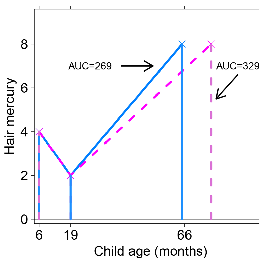
Relationship between hair mercury and age for two hypothetical subjects during the early childhood period. Enclosed areas represent cumulative or AUC Hg values for the corresponding subject.

2.2. Application of the methods to the Seychelles Child Development Study

2.2.1. Overview of our approach

We use multiple measurements of postnatal Hg in the SCDS Main Cohort to develop our method. Our approach has two basic steps: imputing missing Hg values for individual participants at the subset of ages at which it was missing; and creating time-weighted average metrics for each participant during the specific time window of interest. Prior to imputing missing Hg values, we calculate the age- and sex-specific means and standard deviations and the sex-specific pairwise correlations across ages of Hg on the natural logarithmic scale to better inform our imputation process. We use the logarithmic scale for all aspects of the imputation process because in the SCDS at each age Hg levels on the logarithmic scale are more normally distributed than the untransformed values. This was also noted in other studies of Hg exposure (Budtz-Jorgensen et al 2004). We take the following steps to impute missing Hg values: (1) for each age, choose the three most similar ages to use for imputation; (2) calculate imputed Hg for each participant at each age based on decisions from the previous step; (3) evaluate this process by comparing measured and imputed Hg values at each age among participants for whom Hg was measured; and (4) replace missing Hg values with imputed values. We describe the SCDS population in Section 2.2.2, explain our imputation process (e.g., for step 2 above) in Section 2.2.3, describe how we obtain the TW averages in Section 2.2.4, and give our criteria for evaluating both the missing data imputation and the final TW metrics in Section 2.2.5.

2.2.2. Study population

The SCDS Main Cohort enrolled 779 mother-child pairs in 1989-1990 at 6 months (+/− 2 weeks) of age in order to examine the impact of prenatal Hg exposure from fish consumption on children’s neurodevelopment (Davidson et al., 1998). Our focus in this analysis is on postnatal Hg exposure. However, the prenatal period was chosen to be one of the three closest ages to the 6-month visit and used only to impute postnatal Hg at 6 months (see Section 3.2). Multiple test batteries of neurodevelopment and other outcomes were administered to the children at ten ages: 6, 19, 29, and 66 months (i.e., 5.5 years), and 9, 10.5, 17, 19, 22, and 24 years (van Wijngaarden et al. 2017). We conducted all evaluations during increasingly wide time windows with the later evaluations being within +/− 1 year. We collected hair from most cohort children at each visit except at 29 months and 10.5 years, and measured postnatal Hg in the child’s hair in the 1 cm closest to the scalp as an estimate of concurrent MeHg exposure. In the SCDS over 80% of the Hg in hair is in the organic methylated form (Davidson et al., 1998). Although we collected hair at 9 years, many boys had shaved their heads. Consequently, 90% of the girls but only 48% of the boys had a 9-year Hg value. Therefore, we do not directly consider the 9-year Hg measurement in creating our metrics, but we do use it when imputing missing postnatal values.

The seven ages at which postnatal hair was used to create time-weighted averages span two time windows: 6 to 66 months (the childhood period), and 17 to 24 years (early adulthood). The rate of brain development is far more rapid during the early childhood period than in early adulthood (Dobbing and Sands, 1979), so Hg exposure in early adulthood may have a different impact on neurodevelopment than the same exposure in childhood. In addition, due to the large gap between 66 months and 17 years we create separate time-weighted exposure metrics in these two periods. We refer to the TW metric in childhood as TW-C, and the TW metric in early adulthood as TW-A.

Our goal was to collect hair samples at the same set of ages for all participants, but missed appointments, logistics, funding, scheduling and other considerations inherent to observational studies led to the actual participant ages varying somewhat around the intended age. For example, at the 5.5-year visit, the age range at which the children were seen was 5.44 to 6.44 years. At the 24-year visit, the age range was 24.16 to 25.70 years. We use information about the participants’ ages when developing our metrics.

2.2.3. Addressing missing Hg values

Missing Hg measurements usually occurred because participants missed their appointments. Table 1 shows the number of observed and missing Hg values at each visit and at different combinations of visits. Among the 779 participants enrolled, 33 did not have prenatal Hg measured; some of these 33 had postnatal Hg measurements. There were 770 participants who had at least one Hg measurement during the early childhood period and 621 (80.6%) had Hg values at all three of these ages. Among the 677 participants whose Hg was measured during at least one of the early adulthood ages 383 (56.6%) had all four Hg measures. Our goal here is to utilize all the data available to obtain the best estimate of their exposure during the relevant time span. To accomplish this, we first impute missing Hg at all ages for nearly all participants.

Table 1:

Distribution of the number of Hg measurements at each visit age and at combinations of ages among the n=779 SCDS Main Cohort participants.

Age	number missing	number observed
Prenatal (maternal)	33	746
6 months	83	696
19 months	40	739
66 months	71	708
9 years	242	537
6, 19, and 66 months		621
6, 19, or 66 months		770
17 years	215	564
19 years	298	481
22 years	212	567
24 years	203	576
17, 19, 22, and 24 years		383
17, 19, 22, or 24 years		677

Our imputation of missing Hg at a particular age is based on observed Hg values for the same participant at other ages and information about sex-specific Hg means among other participants at the age for which the Hg value was missing. To carry out the imputation, we take the following steps that we describe in more detail below: (1) create age- and sex-specific Z-scores of measured Hg on the natural logarithmic scale at each age; (2) create an imputed Z-score for each participant at each age; (3) back-transform the imputed Z-scores to obtain imputed Hg values on the logarithmic scale; (4) create a final “observed-imputed” log(Hg) value . We refer to our imputation process as an “average Z-score method”.

Calculating Z-scores in step 1 puts the log(Hg) values on a comparable scale across ages and sexes. Using Hg on the natural logarithm scale, our calculated Z-score at a particular age in step 1 is defined as the observed log (Hg) value minus the age- and sex-specific mean, divided by the age- and sex-specific standard deviation. This method of creating Z-scores means that for any two ages, the sex-specific correlations between Z-scores is identical to the sex-specific correlation between the log(Hg) values at the same ages. However, unlike log(Hg), the Z-scores have a mean of 0 and standard deviation of 1 for each sex at each visit age, which makes their distributions directly comparable at all ages. Consequently, in step 2 we impute a participant’s estimated Z-score at a particular age as the average of their Z-score over the three similar ages as described in Section 3.2. We refer to this imputed value as the imputed Z-score. When Hg was only measured at 1 or 2 of these three ages, the imputed Z-score is the average Z-score over those 1 or 2 observed Z-scores; evaluation of this decision is addressed in Section 3.2.

We then calculate the imputed log(Hg) at each age by rescaling the Z-scores at each age to match the original age- and sex-specific mean and standard deviation (SD). We do this by multiplying the Z-scores by the age- and sex-specific SD of log(Hg) and then adding the age- and sex-specific log(Hg) mean. We call this the “back-transformed” imputed log(Hg) value. If desired, we can exponentiate log(Hg) to get Hg on the original scale. Having values of imputed Hg at each age allows us to evaluate how well our imputation process performs in relation to observed Hg values at each age, since we calculate an imputed Hg value for participants for whom Hg was measured, as well as for those with missing Hg. The final log(Hg) value used in the time-weighted Hg metrics is the log(Hg) from the observed value, when measured, and is the back-transformed imputed log(Hg) value otherwise.

2.2.4. Development of time-weighted (TW) Hg metrics

After imputing missing values, we develop TW exposure metrics. These metrics require information about the age of each participant at each visit during the age span of interest. Generally, when a participant’s Hg was missing they were also not seen by the study team so their age at that visit was also missing. In these cases, we imputed their visit age as the average age of the other participants at that visit.

As previously noted, our calculation of the TW average uses log(Hg) when measured, and uses the back-transformed imputed log(Hg), as defined in Section 2.2.3, otherwise. Our TW-C metric is based on Hg at 6 months, 19 months, and 5.5 years, and is the weighted geometric mean of these three Hg values. Specifically, to obtain the TW-C metric, we first calculate the subject-specific geometric Hg averages during the two time windows: (i) 6 to 19 months, and (ii) 19 months to 5.5 years. We then take a weighted average of these two numbers, weighting each by the subject-specific proportion of time spanned by the corresponding time window, relative to the total time spanned by the metric.

To illustrate this calculation, we return to the example of two hypothetical participants illustrated in Figure 1, for whom we calculated the childhood AUC by the traditional method in Section 2.1.2. Using our proposed method, the Hg values of 4, 2, and 8 for both subjects become 1.3863, 0.6931, and 2.0794 on the natural logarithmic scale, giving average log(Hg) values in the first and second time window of 1.0397 and 1.3863 respectively. When exponentiated, the geometric means are 2.828 and 4.000. For the first subject, seen at 6, 19, and 65 months, the weight given to the first time window is (19-6)/(65-6)=0.2203, and the weight for the second time window is 0.7797. For the second subject, seen at 6, 19, and 77 months, the weights are 0.1831 and 0.8169. The TW-C metric in childhood for the first subject is 0.2203 * 2.828 + 0.7797 * 4 = 3.742. Similar calculations for the second subject give a TW-C metric of 3.785. The TW-C for the second subject is 1.2% larger than the first subject, far smaller than 22% as was the case for the AUC metric (see Section 2.1.2). The time window of interest (6 to 66 months) is the same for both subjects. This calculation shows that the AUC metric is far more sensitive than the TW-C to measurements taken far outside the desired time window.

For the TW-A metric, we use observed or imputed log(Hg) values from 17, 19, 22, and 24 years. Since this age range is divided into three time periods (17-19 years, 19-22 years, and 22-24 years), the TW average log(Hg) for the early adulthood period is a weighted average of three average log(Hg) values, where the weights are calculated in the manner as just described. We follow similar steps for weighting the average log(Hg) values in each of these three time periods, and then exponentiate the final TW average log(Hg) value to get our TW-A measure.

2.2.5. Criteria for evaluating imputed mercury values and overall metrics

Our criteria for a better metric based on exposure from multiple ages includes the following: (1) the measured and imputed values for missing Hg data are closer than competing methods; (2) it maximizes the number of participants for whom the overall exposure metric can be calculated; and (3) the final metric accounts for measurement ages that differ across subjects, and for different time spans between consecutive ages.

For our first criterion we compare the performance of seven imputation processes: our average Z-score method, the AUC metric, an arithmetic average exposure metric, a geometric average exposure metric, and three variations of the FCS method. In this comparison, we imputed Hg at 19 months, and separately at 19 years, under each method for all participants who had Hg measured at the age of interest (19 months, or 19 years) and at the three similar ages used for imputation under our method. This ensures the same sample size for all imputation methods at a given age.

For the AUC and average exposure metrics, missing data at a particular age are usually not considered. However, for the average exposure metric ignoring missing data is equivalent to imputing the missing value by replacing the missing exposure with the participant-specific average exposure (using either the arithmetic or geometric mean) over the relevant age range. Equivalence here means that substituting a missing value with the imputed value results in the same average exposure as when the missing value is ignored.

For the AUC metric, when data are missing at any age except the very first and last ages in the age range, equivalence is achieved when missing exposure is interpolated, i.e. it is imputed as a weighted average of observed exposure just prior to and just after the age at which it is missing. This weighted average is the same as the value that would be obtained after drawing a straight line between these two observed values in a plot of Hg versus age, and estimating missing exposure as the value on the line for the age in which exposure is missing. This method was used implicitly in Myers et al (2009).

Although the FCS method is generally used to impute multiple values of missing data, here we use it to impute a single value, consistent with our goal. To be most comparable with our average Z-score method we impute log(Hg) values, and then exponentiate it. We compare three FCS variants. One uses a single FCS imputation based on child sex and log(Hg) at all 9 ages, which we call “FCS-9 single.” The second is the predicted (i.e. mean) value from this same FCS imputation, which we call “FCS-9 mean”, and the third, which we call “FCS-4 mean” is the predicted value from FCS using sex and log(Hg) at four ages - the imputation age and the three similar ages used for the TW metric imputation. Others have noted overfitting and/or collinearity issues of the FCS method when a large number of correlated measures are included in the model (Huque et al., 2018).

Imputation of missing Hg at a particular age under the FCS method uses information about measured Hg from other participants at that same age, as well as covariates and Hg at other ages as specified by the user. The Multiple Imputation for Chained Equations (MICE) computing software for FCS in the R software only performs imputation for missing values. This makes it impossible to compare observed and imputed Hg, without artificially setting to missing some Hg values at the age of interest. In order to fairly compare FCS metrics to the TW metric, for both metrics we set Hg values at the age of interest to missing for half the cohort. We then imputed these values based on Hg at that age from the other cohort half, as well as child sex and Hg at other ages from the entire cohort. Finally, we repeated the process to impute missing data for the other half of the cohort.

Our measures of performance are the mean difference and sum of squared differences between the imputed values and the observed values at that age, where small values indicate closer agreement between observed and imputed values and therefore better performance.

3. Results

3.1. Sample sizes and mercury values

In Table 2 we show the distribution of the number of SCDS participants with 0, 1, 2, or 3 observed Hg measurements that can be used for the childhood and the early adulthood time periods. Only 9 participants did not have Hg measurements in any of the three childhood ages. For these 9 participants we set the childhood TW Hg metric to missing, leaving n=770 participants for whom our childhood TW metric was calculated. 102 participants had no Hg measurements at any of the four later time periods, leaving n=677 participants for whom we calculated the early adulthood TW metric.

Table 2:

Distribution of the number of Hg measurements available for creating time weighted average Hg metrics in the SCDS Main Cohort.

	Number of available measurements
	0	1	2	3	4
6, 19, 66 months	9	18	131	621	-
17, 19, 22, 24 years	102	65	96	133	383

In Figure 2 we show the distribution of log(Hg) for all measured values at each age, separately by sex. Figure 2 shows somewhat of an increase in the median Hg with age from 19 months to 19 years before a substantial decrease at age 22 years. It also shows that starting at 66 months, the difference in mean log(Hg) between the two sexes generally widens with age. Figure 3 shows Hg values over time for a subset of Seychellois boys, chosen to illustrate different missing value patterns. Panel A shows observed Hg values versus age for six boys with no missing Hg values, and panel B shows the relationships for the same boys with Hg transformed to be a Z-score on the logarithmic scale. A comparison of those two panels shows that the distribution of the transformed values is more symmetric and more similar across ages than the measured values. Panel C shows observed Hg values for six other boys for whom Hg was not measured at all ages, and Panel D show the same observed values, where missing values are replaced by the imputed values under our method.

Figure 2:

Boxplots of log(Hg) at each visit age, separately by sex (left: girls, right: boys), among the SCDS Main Cohort participants.

Figure 3:

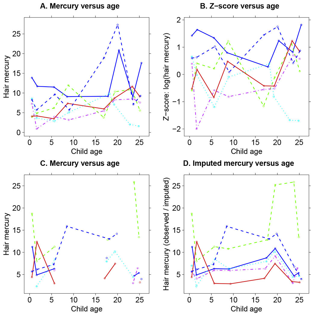
Relationship between hair mercury and age for some SCDS Main Cohort male participants. A: Hg versus age for some participants with fully observed Hg. B: Z-score of log(Hg) versus age for the same participants as in panel A. C: Hg versus age for some participants whose Hg is not fully observed. D: observed or imputed Hg versus age for the same participants as in panel C.

3.2. Imputation of mercury values

Before imputing missing Hg values, we first determined the three similar ages to use for imputation. Correlations between Hg levels were generally larger for two similar ages, and for pairs of ages in the early adolescent period (Table 3). To impute Hg at 6 months we use information from prenatal (i.e., maternal) Hg and the child Hg at 19 months and 5.5 years. For Hg at 19 months, we use 6-month, 5.5 years, and 9-year Hg values, and for 5.5-year Hg we use Hg at 6 months, 19 months, and 9 years. For early adulthood (17, 19, 22, and 24 years), we use Hg at each of the other three ages in this time window. Although neither the TW-C nor the TW-A metric included 9 years due to substantial missing Hg data, for completeness we also imputed 9-year Hg in the same way, using 5.5, 17, and 19-year Hg values. As noted in Section 2.2.3, the imputed value for each participant is based on Hg from as many of these ages as it was measured.

Table 3:

Pairwise correlations of log(Hg) across multiple ages among SCDS Main Cohort participants.

	6 mo	19 mo	66 mo	9 yr	17 yr	19 yr	22 yr	24 yr
Maternal	0.27	0.17	0.10	0.07	0.10	0.13	0.09	0.10
6 mo		0.22	0.20	0.18	0.07	0.03	0.11	0.12
19 mo			0.34	0.16	0.15	0.09	0.10	0.08
66 mo				0.45	0.29	0.21	0.20	0.19
9 yr					0.27	0.28	0.22	0.23
17 yr						0.34	0.36	0.43
19 yr							0.38	0.38
22 yr								0.56

Since Hg values for the imputation process may themselves be missing, we evaluate whether it is reasonable to impute missing Hg for participants who have only one or two Hg measurements at the three similar ages used to calculate imputed Hg at the relevant age. Using Hg on the log scale throughout, at each age we calculated the correlations between measured Hg and imputed Hg. We did this first for all participants who have at least one of the three Hg measures at the three similar ages (columns labeled “Any # measures” in Table 4). We then repeat this after stratifying by whether the participant had one, two, or all three Hg measurements at these three similar ages. For example, among the 695 participants who had a measure of both 6-month Hg and Hg for at least one of three similar ages (maternal prenatal, 19 months, and 66 months, in this example) the correlation between the measured 6-month Hg and the imputed 6-month Hg is 0.36. Among these 695 participants, 621 had Hg at all three of these similar ages.

Table 4:

Correlations between measured log(Hg) and imputed log(Hg) at each visit age among SCDS Main Cohort participants, stratified by the number of measured Hg values available at the three similar ages identified for calculating the imputed Hg value at that age.

	Any # measures		3 measures		2 measures		1 measure
	n	corr	n	corr	n	corr	n	corr
6 months	695	0.36	621	0.34	39	0.41	35	0.56
19 months	736	0.35	449	0.29	239	0.47	48	0.30
66 months	706	0.44	449	0.47	227	0.42	30	0.37
9 years	513	0.47	356	0.47	86	0.43	71	0.49
17 years	541	0.45	383	0.45	112	0.50	46	0.36
19 years	476	0.45	383	0.50	63	0.27	30	0.24
22 years	555	0.57	383	0.58	112	0.58	60	0.43
24 years	551	0.60	383	0.59	112	0.65	56	0.50

Among these 621 participants the correlation between the observed and imputed 6-month Hg is 0.34. Also 39 had a measurement of Hg from two of the three similar ages, for which the correlation between observed and imputed Hg is 0.41. Finally, among the 35 participants with a single measured Hg value at the three similar ages, the correlation between observed and imputed Hg is 0.56.

For the childhood period the correlations between measured and imputed values are almost identical or even slightly greater among participants for whom the imputed value was based on Hg at a single age as compared to three ages. In early adulthood (17, 19, 22, and 24 years) the correlations were lower when imputation was based on Hg at a single age as compared to three ages, but except for the 19-year Hg values, the correlations were similar. We conclude that imputation for missing Hg at a specific age could reasonably be based on as Hg measured from as few as one of three similar ages, and was preferable to a substantial reduction in sample size if we were instead to set this value to missing.

In Table 5 we show the sample size, mean and SD of measured untransformed Hg at each age (“observed” in row labels) separately by sex. We also show the sample sizes and sex-specific mean and SD of the Hg values used to construct the TW metrics (“obs/imputed” in row labels). The latter rows use measured Hg values when available, and imputed Hg values otherwise. There is a substantial increase in sample size when missing values are imputed, particularly for the early adulthood ages. Consistent with Figure 2, the mean Hg values are fairly similar for boys and girls at the three childhood ages, although at 6 months the mean for boys is slightly larger and at 19 months the mean for girls is slightly larger. For all four of the early adulthood ages, the average Hg value for males was substantially larger than females. The sex- and age-specific means of the Hg values used in our models (“obs/imputed” in row labels) were very similar to the observed Hg values for the corresponding age and sex, suggesting that our average Z-score method of imputation preserved the age- and sex-specific Hg distributions within each time period.

Table 5:

Means (SDs) of observed Hg (ppm) and observed / imputed Hg values at each visit age in the SCDS Main Cohort, separately for boys and girls. Rows with a label of “(obs / imputed)” use the observed Hg value if available, and the imputed value otherwise. The p-values are from t-tests of whether the mean of each Hg variable differs by sex.

	Total	Female		Male
	n	n	Mean (SD)	n	Mean (SD)	p
Maternal Hg	746	369	6.94 (4.51)	377	6.67 (4.49)	0.42
6M Hg (observed)	696	349	6.31 (4.02)	347	6.92 (4.77)	0.07
6M Hg (obs/imputed)	770	383	6.28 (3.9)	387	6.9 (4.58)	0.04
19M Hg (observed)	739	372	5.07 (3.25)	367	4.54 (2.85)	0.02
19M Hg (obs/imputed)	770	383	5.12 (3.28)	387	4.58 (2.84)	0.02
66M Hg (observed)	708	352	6.66 (3.25)	356	6.34 (3.39)	0.21
66M Hg (obs/imputed)	770	383	6.59 (3.19)	387	6.27 (3.34)	0.17
9Y Hg (observed)	537	348	5.93 (3.44)	189	6.48 (3.78)	0.1
9Y Hg (obs/imputed)	742	375	5.91 (3.43)	367	6.31 (3.73)	0.13
17Y Hg (observed)	564	311	7.28 (4.3)	253	9.09 (4.92)	0.00
17Y Hg (obs/imputed)	677	345	7.16 (4.26)	332	9.03 (4.85)	0.00
19Y Hg (observed)	481	273	8.65 (4.68)	208	12.45 (6.94)	0.00
19Y Hg (obs/imputed)	677	345	8.59 (4.6)	332	12.54 (6.47)	0.00
22Y Hg (observed)	567	311	4.03 (3.58)	256	6.56 (4.05)	0.00
22Y Hg (obs/imputed)	677	345	3.91 (3.48)	332	6.52 (3.9)	0.00
24Y Hg (observed)	576	313	3.81 (2.76)	263	6.33 (4.23)	0.00
24Y Hg (obs/imputed)	677	345	3.77 (2.69)	332	6.31 (4.13)	0.00
Childhood (6M-66M) TW metric	770	383	5.48 (2.6)	387	5.16 (2.47)	0.08
Early adulthood (17Y-24Y) TW metric	677	345	5.62 (3.05)	332	8.7 (4.08)	0.00

3.3. Resulting TW metrics

In the last few lines of Table 5 we show the distribution of our TW metrics. The mean TW metric in childhood was somewhat larger for girls (mean=5.48 ppm, SD=2.60) than boys (mean=5.16 ppm, SD=2.47). In early adulthood the differences in the TW means for the two sexes is even more pronounced. Across the entire 7-year early adulthood age span, the mean TW exposure metric was 5.62 ppm (SD=3.05) for females and 8.70 ppm (SD=4.08) for males.

3.4. Evaluation of imputed mercury values and overall metrics

3.4.1. Criterion 1: similarity of measured and imputed values for missing Hg data

Our first criterion for a better metric is whether imputed Hg values are more similar to the observed values than other methods. Our comparison of the seven imputation methods first evaluates their performance at 19-months using data from the 621 participants who had Hg measures at all three childhood ages, and then at 19 years using data from the 379 participants who had Hg measures at all four of the early adulthood ages. Our evaluation is based on comparing the absolute value of the mean difference between the imputed and measured Hg values (the bias), and the sum of squared (SS) differences between the imputed and measured Hg, with smaller values indicating better performance. We first compare the AUC metric, the arithmetic and geometric average, and our average Z score method at 19 months.

As shown in Table 6, by these criteria our average Z-score method performed considerably better than the AUC and average exposure metrics. At 19 months, our average Z-score method underestimated the measured 19-month value by 0.50 ppm on average, whereas the three competing methods overestimated the 19-month value by 1.24 to 1.60 ppm, making their absolute bias 2.5 to 3.3 times greater than our average Z-score method. The sum of squared differences between the imputed and observed Hg for all three competing methods were larger than our TW metric, by a factor ranging from 1.28 to 1.49.

Table 6:

Performance of competing methods to impute missing Hg data at 19 months and at 19 years among SCDS Main Cohort participants, based on a comparison of imputed values to observed Hg values. For each method, table entries show mean differences, sum of squared (SS) differences, and the ratio of the mean differences (in absolute value) and SS differences to the average Z-score method. Comparisons are based on the subset of n = 621 participants in early childhood and n = 379 in early adulthood who have complete Hg data at all ages within the time window.

	Average Z-score	Average	Geometric average	AUC	Average Z-score*	FCS-9 single*	FCS-9 mean*	FCS-4 mean*
19 months
Mean difference	−0.50	1.64	1.24	1.60	−0.38	0.25	−0.72	−0.79
SS differences	6278	9378	8016	8717	6337	10,068	5705	5564
Mean ratio†	–	3.30	2.50	3.22	–	0.65	1.90	2.08
SS ratio†	–	1.48	1.26	1.38	–	1.59	0.90	0.88
19 years
Mean difference	−0.65	−4.31	−4.96	−4.16	−0.56	0.25	−1.01	−1.07
SS differences	10,004	16,142	18,572	16,109	10,419	18,945	10,415	10,314
Mean ratio†	–	6.60	7.59	6.37	–	0.44	1.78	1.87
SS ratio†	–	1.55	1.78	1.55	–	1.82	1.00	0.99

^*Imputation uses Hg data at the age of interest from 50% of the sample.

^†Denominator for ratio calculation is average Z-score; the mean ratio is an absolute value

As described in Section 2.2.5, since the FCS method only imputes Hg when it is missing, we used information from 50% of the 19-month Hg data at a time for the FCS imputation. We used the same 50% of the Hg data for our average Z-score method when comparing it to the FCS method (Table 6). Results from the FCS method that imputed a single value based on child sex and all 9 Hg values (“FCS-9 single”) were closer on average than the average Z-score method, but the sum of squared differences under “FCS-9 single” was considerably larger than all other methods. The FCS methods that impute the mean value, either based on child sex and all 9 Hg values (“FCS-9 mean”) or sex and 4 Hg values (“FCS-4 mean”) gave estimated values that were substantially more biased than the average Z-score method, but less biased than the AUC or average exposure metrics. Compared to the average Z-score method, the sum of squared differences were smaller for the FCS mean imputations, a fact that can be attributed to the smaller overall variance of these imputed values compared to the observed 19-month Hg.

The performance of four of these methods can be compared visually in in Figure 4. Each panel shows the imputed 19-month Hg versus the observed 19-month Hg, with imputation using the AUC (Panel A), the average Z-score method (Panel B), the FCS-9 mean (Panel C) and the FCS-9 single method (Panel D). The diagonal line is the 1:1 line. Panel A shows that the AUC metric tends to overestimate 19-month Hg, while Panel C shows the FCS-9 mean tends to underestimate 19-month Hg. The small biases in the average Z-score and the FCS-9 single methods are not visibly discernable (Panels B and D).

Figure 4:

Relationships between estimated and measured Hg at 19 months in the SCDS Main Cohort. Estimates for the average Z-score and FCS methods are based on setting 50% of the 19-month Hg data to missing.

At 19 years, our TW metric underestimated the measured Hg values by 0.65 ppm on average. In contrast, the AUC and both average metrics underestimated the measured Hg value by more than 4.00 ppm. Furthermore, the sum of squared differences between imputed and measured Hg values of the AUC, both average metrics, and FCS-9 single were 61% to 86% larger than our average Z-score. The mean difference between the imputed and observed 19-year Hg value was the smallest using the FCS-9 single metric. However, the SS difference using this metric was 1.82 times larger than under our average Z-score method. The two FCS mean metrics were more biased than the average Z-score by a factor of 1.78 to 1.87, while having almost identical sum of squared differences as the average Z-score.

The performance of four methods for estimating 19-year Hg is shown in Figure 5. The underestimation of the observed value by the AUC metric (Panel A) is visibly discernable, while the smaller bias in the average Z-score (Panel B), FCS-9 mean metric (Panel C) and the FCS-9 single metric (panel D) is less evident. The larger variability of the FCS-9 single relative to the other metrics is also discernable.

Figure 5:

Relationships between estimated and measured Hg at 19 years in the SCDS Main Cohort. Estimates for the average Z-score and FCS methods are based on setting 50% of the 19-year Hg data to missing.

3.4.2. Criterion 2: maximize number of participants for whom the metric can be calculated

Our second criterion addresses the number of participants for whom a long-term metric can be calculated. The FCS method is not relevant here, since FCS is a method for imputing data but not a method to combine multiple exposure measures. The two average exposure metrics and our TW metric can be obtained for all participants with at least one exposure measure in the age range of interest, namely n=770 for the childhood period and n=677 in early adulthood. The AUC metric as usually defined does not handle missing exposure at the earliest and latest ages of interest; both would need to be measured. In the SCDS data, an AUC metric for the childhood period would require measurements of Hg at 6 months and 5.5 years, but the 19-month Hg data could be missing. 638 participants met this criterion: 621 with Hg at all three time points, and 17 with 6-month and 5.5-year Hg but no measurement of 19-month Hg. An AUC metric for the early adulthood period would require Hg measurements at 17 and 24 years, a criterion that is met for 483 participants: 383 with Hg at all time points, and 100 missing only 19-year and/or 22-year Hg. Since the TW metric and an average exposure metric can be created for more participants than an AUC metric, these two metrics better meet our second criterion than the standard AUC. It should be noted that a modified AUC metric could be defined in which missing exposure at the first and last time points could be imputed. This modified metric would also do well under our second criterion.

3.4.3. Criterion 3: account for different measurement ages when creating final metric

Our third criterion addresses which metric best accounts for different time spans between measurements and varying ages at each measurement time. As described earlier, both the TW metric and an AUC metric take into account the time periods between adjacent measurements, whereas an average exposure measure does not. In Section 2.1.2 we noted that the AUC metric is not optimal when the age span of interest is the same for all participants, but the measured ages at the first and last ages vary across participants. In this case the AUC metric will be artificially influenced by the difference in first and last ages, and will on average be larger for participants with a large age span relative to those with a smaller age span. Therefore, we argue that the TW metric better satisfies our third criterion than either the AUC or average exposure metric.

4. Discussion

In this paper we addressed two questions that arise when creating a long-term exposure metric for any toxicant using Hg as a model: how to address missing exposure data, and how to combine multiple exposure measurements into a single metric. As is typical in longitudinal cohort studies, not all SCDS participants had a measured Hg value at all ages of interest. We imputed Hg for an individual participant at a specific age by averaging Z-scores using information from the participant’s measured Hg values at similar ages, and from sex-specific Hg means (on the natural logarithmic scale) for other individuals at this age. Except for the 102 participants (13.1%) who had no Hg measurements at any of the four early adulthood ages, we were able to impute missing Hg values in the vast majority of cases. This allowed us to utilize all the available data and determine a more complete picture of each participant’s longitudinal Hg exposure.

Once we have imputed missing exposure data, we used our method of combining repeated exposure measurements in a pre-defined age range to obtain a single measure of long-term exposure in this a specific age window. Our novel exposure metric is a time-weighted (TW) metric of average toxicant exposure over the age range of interest, using measured exposure when available, and imputed exposure using our average Z-score method otherwise. We show that the TW metric is applicable when the age range of interest is the same for all participants, and can be used when measurement ages are not equally spaced. We created two TW Hg metrics, one in childhood representing average Hg exposure from 6 months to 5.5 years (TW-C) and the other an early adulthood metric using Hg measured from 17 to 24 years (TW-A).

Other authors have also compared methods for imputing missing data for a covariate measured at more than one time point. Karahalios et al (2013) evaluated methods for addressing missing data using simulated data based on the Melbourne Collaborative Study. Their Interest focused on estimating the risk of colorectal cancer in relation to waist circumference compared to baseline. The authors concluded that there is no advantage in using multiple imputation over a complete case analysis, when the missing data mechanism is not associated with the outcome. Kalaycioglu et al. (2016) used simulation to compare a variety of multiple imputation methods for time-varying covariates that are missing at random. They found that results from FCS were sensitive to the correlation between repeated measurements. De Silva et al (2017) also used simulation to examine the performance of two FCS models and a multivariate normal model for imputing missing data in a time-varying covariate (Z-scores of BMI) that has a nonlinear association with age. All methods designed to address missing data performed well in their simulation.

Our method of imputing missing exposure data is similar to the FCS extension that imputes missing data only using information from the same or adjacent time periods (Nevalainen at al. 2009). Welch et al (2014) compared results from the FCS method to results in which data was imputed using data from all time blocks (which often did not run successfully), or only using data from the first time block. The FCS imputation showed a gain in efficiency, but only for time-dependent variables. Our method of imputing missing Hg data differs from this FCS extension because (a) we use information from more ages than this version of the FCS method to impute missing values; (b) we impute missing data by averaging Z-scores rather than from a regression model; and (c) we do not impute missing data iteratively or multiple times.

Our results indicate that ignoring missing exposure data in a long-term metric, such as is typical in the AUC and average exposure metric, may induce bias. This is particularly the case when average exposure varies across age and/or across levels of another covariate such as sex. In this case, bias can be reduced when these systematic differences are taken into account appropriately during the imputation process.

The method we use to impute missing exposure has several strengths. Imputing missing Hg values by averaging Z-scores allows any number of Z-scores of repeated exposure to be averaged without inducing collinearity. In contrast, imputing missing data in a regression in which the covariates include exposure at multiple time periods, such as FCS, leads to increasing collinearity as the number of exposure variables increases. Our use of a time-weighted average in developing the final TW exposure metric makes appropriate use of the age gaps between exposure measurements, as does the AUC. Our method is not directly affected by differences in participant’s ages at the earliest and latest age window of interest, whereas these differences can introduce extraneous variability into the AUC metric. In addition, the TW metric does not require exposure to be measured at the earliest and latest ages, unlike a standard AUC metric. A further strength in this paper is the availability of postnatal Hg measurements at many ages on the majority of the participants in the SCDS, which is unusual among studies of long-term exposure. This rich source of exposure data was important in allowing us to create and evaluate our exposure metrics.

Our method of imputing missing Hg and creating overall TW metrics also has some limitations. In contrast to the FCS extension where any number of covariates at a particular age can easily be incorporated for the imputation model, we chose to use only age and sex to help predict missing Hg. This is not an inherent limitation to the average Z-score method because we could have incorporated other covariates for the imputation. A further limitation is that creating a single TW metric for each participant for each age range of interest ignores the uncertainty due to imputing missing Hg values. However, our ultimate goal is to create metrics of time-weighted average Hg, and not individual Hg values at a particular age. For each time period, the TW metric for all participants is always based on at least one observed Hg value. Consequently, the uncertainty due to missing individual Hg values translates into a much smaller uncertainty once the imputed Hg values are incorporated into an overall TW average.

If FCS is used to impute a single value of each missing Hg measurement, we suggest using the best estimate (e.g. the predicted value), which minimizes variability of the final estimate compared to using the predicted value plus error (a single imputation). However, in the SCDS data the FCS method that imputes the single best estimate of Hg at 19 months or 19 years had nearly double the absolute bias of our average Z-score method for imputation. One reason for the better performance of our method is that by averaging subject-specific Z-scores, our method implicitly accounts for larger or smaller average exposure levels among individual subjects. These subject-specific differences cannot be fully captured by a regression model, such as used in the FCS method.

The metrics developed here extend our earlier work and provide additional advantages including being able to incorporate information from many participants with missing exposure data. These time-weighted average Hg measures will be useful in subsequent studies to examine associations between postnatal Hg exposure and multiple longitudinal neurodevelopmental outcomes in this cohort. These metrics have already been used to examine associations with 85 SCDS Main Cohort neurodevelopmental outcomes measured between ages 9 to 24 years (Thurston et al., 2022), where several statistically significant adverse associations were noted.

5. Conclusions

We developed two time weighted Hg exposure measures to reflect childhood and young adult exposures over time when faced with some missing Hg measurements. These metrics reduce bias and improve accuracy compared to other metrics. The methods presented here are applicable to any study of the effects of long-term toxicant exposure for which longitudinal measurements of the toxicant are available but may have a substantial proportion of missing values.

Bibliography

- Budtz-Jørgensen E, Grandjean P, Jørgensen PJ, Weihe P and Keiding N, 2004. Association between mercury concentrations in blood and hair in methylmercury-exposed subjects at different ages. Environmental research, 95(3), pp.385–393. [DOI] [PubMed] [Google Scholar]
- Chen YH, Ferguson KK, Meeker JD, McElrath TF and Mukherjee B, 2015. Statistical methods for modeling repeated measures of maternal environmental exposure biomarkers during pregnancy in association with preterm birth. Environmental Health, 14(1), p.9. [DOI] [PMC free article] [PubMed] [Google Scholar]
- Davidson PW, Myers GJ, Cox C, Axtell C, Shamlaye CF, Sloane-Reeves J, Cernichiari E, Needham L, Choi A, Wang Y and Berlin M, 1998. Effects of prenatal and postnatal methylmercury exposure from fish consumption at 66 months of age: the Seychelles Child Development Study. JAMA, 280(8), pp.701–707. [DOI] [PubMed] [Google Scholar]
- De Silva AP, Moreno-Betancur M, De Livera AM, Lee KJ and Simpson JA, 2017. A comparison of multiple imputation methods for handling missing values in longitudinal data in the presence of a time-varying covariate with a non-linear association with time: a simulation study. BMC medical research methodology, 17(1), p.114. [DOI] [PMC free article] [PubMed] [Google Scholar]
- Dobbing J and Sands J, 1979. Comparative aspects of the brain growth spurt. Early human development, 3(1), pp.79–83. [DOI] [PubMed] [Google Scholar]
- Ferguson KK, Rosen EM, Barrett ES, Nguyen RH, Bush N, McElrath TF, Swan SH and Sathyanarayana S, 2019. Joint impact of phthalate exposure and stressful life events in pregnancy on preterm birth. Environment international, 133, p.105254. [DOI] [PMC free article] [PubMed] [Google Scholar]
- Hornung RW, Lanphear BP and Dietrich KN, 2009. Age of greatest susceptibility to childhood lead exposure: a new statistical approach. Environmental Health Perspectives, 117(8), pp.1309–1312. [DOI] [PMC free article] [PubMed] [Google Scholar]
- Huque MH, Carlin JB, Simpson JA and Lee KJ, 2018. A comparison of multiple imputation methods for missing data in longitudinal studies. BMC medical research methodology, 18(1), pp.1–16. [DOI] [PMC free article] [PubMed] [Google Scholar]
- Kalaycioglu O, Copas A, King M and Omar RZ, 2016. A comparison of multiple-imputation methods for handling missing data in repeated measurements observational studies. Journal of the Royal Statistical Society: Series A (Statistics in Society), 3(179), pp.683–706. [Google Scholar]
- Kane HS, Schetter CD, Glynn LM, Hobel CJ and Sandman CA, 2014. Pregnancy anxiety and prenatal cortisol trajectories. Biological psychology, 100, pp.13–19. [DOI] [PMC free article] [PubMed] [Google Scholar]
- Karahalios A, Baglietto L, Lee KJ, English DR, Carlin JB and Simpson JA, 2013. The impact of missing data on analyses of a time-dependent exposure in a longitudinal cohort: a simulation study. Emerging themes in epidemiology, 10(1), pp.1–11. [DOI] [PMC free article] [PubMed] [Google Scholar]
- Kriebel D, Checkoway H and Pearce N, 2007. Exposure and dose modelling in occupational epidemiology. Occupational and environmental medicine, 64(7), pp.492–498. [DOI] [PMC free article] [PubMed] [Google Scholar]
- Little RJ and Rubin DB, 2019. Statistical analysis with missing data (Vol. 793). John Wiley & Sons. [Google Scholar]
- Myers GJ, Thurston SW, Pearson AT, Davidson PW, Cox C, Shamlaye CF, Cernichiari E and Clarkson TW, 2009. Postnatal exposure to methyl mercury from fish consumption: a review and new data from the Seychelles Child Development Study. Neurotoxicology, 30(3), pp.338–349. [DOI] [PMC free article] [PubMed] [Google Scholar]
- Nevalainen J, Kenward MG and Virtanen SM, 2009. Missing values in longitudinal dietary data: a multiple imputation approach based on a fully conditional specification. Statistics in Medicine, 28(29), pp.3657–3669. [DOI] [PubMed] [Google Scholar]
- Rubin DB, 1976. Inference and missing data. Biometrika, 63(3), pp.581–592. [Google Scholar]
- Rubin DB, 1977. Formalizing subjective notions about the effect of nonrespondents in sample surveys. Journal of the American Statistical Association, 72(359), pp.538–543. [Google Scholar]
- Rubin DB, 1987. Multiple imputation for nonresponse in surveys John Wiley & Sons. [Google Scholar]
- Rubin DB, 1996. Multiple imputation after 18+ years. Journal of the American statistical Association, 91(434), pp.473–489. [Google Scholar]
- Schafer JL and Olsen MK, 1998. Multiple imputation for multivariate missing-data problems: A data analyst’s perspective. Multivariate behavioral research, 33(4), pp.545–571. [DOI] [PubMed] [Google Scholar]
- Thurston SW, Myers G, Mruzek D, Harrington D, Adams H, Shamlaye C and van Wijngaarden E, 2022. Associations between time-weighted postnatal methylmercury exposure from fish consumption and neurodevelopmental outcomes through 24 years of age in the Seychelles Child Development Study Main Cohort. NeuroToxicology, 91, pp.234–244. [DOI] [PMC free article] [PubMed] [Google Scholar]
- van Buuren S Multiple imputation of discrete and continuous data by fully conditional specification. 2007. Statistical Methods in Medical Research, 16(3):219–242. [DOI] [PubMed] [Google Scholar]
- van Wijngaarden E, Thurston SW, Myers GJ, Harrington D, Cory-Slechta DA, Strain JJ, Watson GE, Zareba G, Love T, Henderson J and Shamlaye CF, 2017. Methyl mercury exposure and neurodevelopmental outcomes in the Seychelles Child Development Study Main cohort at age 22 and 24 years. Neurotoxicology and teratology, 59, pp.35–42. [DOI] [PMC free article] [PubMed] [Google Scholar]
- Welch CA, Petersen I, Bartlett JW, White IR, Marston L, Morris RW, Nazareth I, Walters K and Carpenter J, 2014. Evaluation of two-fold fully conditional specification multiple imputation for longitudinal electronic health record data. Statistics in medicine, 33(21), pp.3725–3737. [DOI] [PMC free article] [PubMed] [Google Scholar]
- Wüst S, Federenko I, Hellhammer DH and Kirschbaum C, 2000. Genetic factors, perceived chronic stress, and the free cortisol response to awakening. Psychoneuroendocrinology, 25(7), pp.707–720. [DOI] [PubMed] [Google Scholar]