Fiscal policy during a pandemic

Abstract

I study the effects of the 2020 coronavirus outbreak in the United States and subsequent fiscal policy response in a nonlinear DSGE model. The pandemic is a shock to the utility of contact-intensive services that propagates to other sectors via general equilibrium, triggering a deep recession. I use a calibrated version of the model that matches the path of the US unemployment rate in 2020 to analyze different types of fiscal policies. I find that the pandemic shock changes the ranking of policy multipliers. Unemployment benefits are the most effective tool to stabilize income for borrowers, who are the hardest hit during a pandemic, while liquidity assistance programs are the most effective if the policy objective is to stabilize employment in the affected sector. I also study the effects of the $2.2 trillion CARES Act of 2020.

1. Introduction

The ongoing COVID-19 outbreak is causing widespread disruption in the world’s advanced economies. Monetary authorities were quick to react, with the Federal Reserve and other major central banks promptly reactivating their 2008–09 Financial Crisis toolkits. Following these steps, fiscal authorities around the globe proceeded to design and implement stabilization packages to help sustain household and firm balance sheets.

In this paper, I adapt a macroeconomic model to simulate the macroeconomic effects of a pandemic and study the effects of different types of fiscal policy instruments. The pandemic is modeled as a sudden stop of a contact-intensive services sector. Through aggregate demand externalities, the shutdown of this sector propagates to the non-services sector. Through balance sheet linkages, it also propagates to the financial sector. The rise in unemployment leads to a wave of defaults, disrupting financial intermediation and amplifying the recession. The pandemic shock results in a large spike in the unemployment rate, as in the data. Borrower households, who derive most of their income from employment and rely on bank credit to fund consumption, are the most affected group. I assume that there is endogenous entry and exit in the affected sector, which means that fluctuations in demand can have persistent effects in this sector’s productive capacity and that the economy does not immediately recover when the pandemic is over.

I calibrate the model to the US on the eve of the pandemic and combine it with data on fiscal outlays to estimate a sequence of “pandemic shocks” that allow the model to match the path of the US unemployment rate in 2020. I then use those estimated shocks to study the effects of fiscal policy and counterfactuals. I study the effects of different types of discretionary fiscal policy: (i) an increase in non-service government purchases, (ii) a decrease in the payroll tax, (iii) an expansion of unemployment insurance (UI), (iv) unconditional transfers, and (v) payment of wages by the government to service firms.

In terms of measuring the effectiveness of different measures, it is not clear that the traditional concept of GDP multiplier is appropriate in this context. The shut down of economic activity is largely intentional and part of pandemic suppression measures, and focus on GDP stabilization could be detrimental to fighting the pandemic. For that reason, I evaluate different policies based on consumption and household income multipliers, which measure the dollar impact of fiscal spending on consumption, and on labor income net of government transfers. I find considerable variation in the distributional effects of different types of policies. Borrowers, who are most affected by the crisis, receive a larger consumption boost from policies that resemble cash transfers, such as an increase in UI benefits. I find that unconditional transfers of the type that are currently being proposed generate similar distributional effects, with the added benefit of potentially less-costly implementation. I find that liquidity assistance to firms has the longest-lasting effects and can be very effective in terms of stabilizing employment in the medium run.

I validate the model calibration by computing fiscal multipliers in the absence of the pandemic shock and showing that they are in line with those that have been estimated in the literature. The model is highly nonlinear, and these fiscal multipliers are extremely state dependent: policies with positive multipliers during the pandemic may generate negative ones in normal times. The ranking of policies in terms of multipliers changes during the pandemic: tax cuts, for example, are more effective in “normal times,” while the UI multiplier becomes larger during the pandemic. Finally, I analyze the aggregate and policy-by-policy fiscal multipliers for the Coronavirus Aid, Relief, and Economic Security (CARES) Act of 2020, the $2.2 trillion coronavirus aid package. As in the baseline model, I find that the expansion of UI and liquidity assistance to firms were the most effective components of the package in terms of stabilizing income and employment, respectively.

Literature The exercise in this paper is very similar to the analysis conducted by Drautzburg and Uhlig (2015) and Taylor (2018) for the American Recovery and Reinvestment Act of 2009, where the authors use a DSGE model to simulate a recession scenario and then consider the effects of a policy package. Faria-e-Castro (2018) conducts a similar analysis while also taking into account financial sector interventions such as the Troubled Asset Relief Program (TARP), among others. In this paper, I mostly abstract from issues related to financial sector interventions.

This paper also contributes to the modeling of a pandemic in a macroeconomic model. Fornaro and Wolf (2020) study how monetary and fiscal policy can be used to respond to the current pandemic by preventing the economy from falling into stagnation traps following persistent negative shocks to productivity growth. A rich literature has emerged embedding epidemiology models in real business cycles models: Eichenbaum et al. (2020b) and Glover et al. (2020), among many others. Since they endogenize the dynamics of the epidemic, their models allow them to study optimal health policy responses. They find that a severe recession, generated by agents’ optimal decision to cut back on consumption and hours worked, helps reduce the severity of their epidemic. My analysis is complementary to theirs: I take the epidemic as exogenous and given and study how a fiscal authority can help stabilize income and consumption during the epidemic.2

More closely related is the work of Guerrieri et al. (2020), who show that supply shocks can generate aggregate effects that “look like” aggregate demand shocks in a multiple-sector, incomplete markets economy under certain conditions. While I study the effects of fiscal policy in the context of a pandemic that is modeled as an aggregate demand shock, I show that a supply shock can generate very similar aggregate effects under parameter conditions that are related to theirs.

Other analyses of fiscal policy in response to the COVID-19 crisis include Bayer et al. (2020) and Elenev et al. (2020), who focus on the effects of transfers to households and firm bailouts, respectively. My model is simpler than theirs in many respects but is more general in others, thus allowing me to analyze a broader set of fiscal policies. Bayer et al. (2020) have a much richer setup in terms of household heterogeneity, which includes idiosyncratic income and unemployment risk. This leads them to find much larger differences in terms of the multipliers of targeted (UI) vs. untargeted (lump-sum) transfers. In this paper, I show that even in the absence of rich household heterogeneity, the multipliers for targeted transfers are larger than those for untargeted ones. Importantly, this result reverts in the absence of the pandemic shock, suggesting that the current model features a significant amount of state dependence. Elenev et al. (2020) focus on fiscal support to distressed firms, and while they do not explicitly compute fiscal multipliers for these interventions, they find a large role for fiscal policy in preventing corporate bankruptcies. This is consistent with the large employment multiplier that I find for liquidity assistance policies.

Section 2 presents the model; Section 3 describes the calibration, the modeling of the pandemic, and the estimation of the pandemic shocks; Section 4 discusses the effects of different fiscal policies in the model; Section 5 estimates multipliers for the different components of the CARES Act of 2020; and Section 6 concludes.

2. Model

Time is discrete and infinite. There are two types of households: borrowers and savers. Financial intermediaries use deposits raised from savers as well as their own retained earnings to finance loans to borrowers. There are two sectors in this economy: a non-services sector ($n$-sector) and a services sector ($a$-sector). Labor markets are frictional in reduced form, and employment is demand-determined in both sectors. A central bank sets the interest rate, and a fiscal authority collects taxes and may undertake different types of discretionary interventions. The model is adapted from Faria-e-Castro (2018), and many of its elements are standard in two-agent New-Keynesian models. For this reason, I mostly focus on what is different.

2.1. Households

There are two types of households in fixed types: borrowers in mass $\chi$ and savers in mass $1-\chi$.

2.1.1. Borrowers, debt, and default

There is a representative borrower family that consists of a continuum of agents $i\in [0,1]$. Each of these agents can be employed in the $n$-sector, employed in the $a$-sector, or unemployed. Let $N_t^{n,b},N_t^{a,b}$ denote the mass of agents in the borrower family working in the $n$- and $a$-sectors, respectively, and let $1-N_t^{a,b}-N_t^{n,b}$ denote the mass of unemployed agents in the borrower family. There is perfect labor mobility between the two sectors.

To generate realistic default rates in the context of a representative agent model, I assume that the members of the borrower household are subject to a combination of a cash-in-advance constraint and liquidity shocks. The borrower family enters the period with a stock of debt to be repaid equal to $B_{t-1}^b$. Each member of the household is responsible for repaying an equal amount $B_{t-1}^b$ at the beginning of the period. At this point, the only available resources are labor income, net government transfers, and a liquidity shock ${\epsilon }_t\left(i\right)\sim F^e,F^u,$ where $F^e,F^u$ are distributions with support in the real line.3 Total cash in hand is therefore given by

$$\mathrm{1}[i\in N_t^{n,b}]w_t(1-{\tau }_t^l)+\mathrm{1}[i\in N_t^{a,b}]w_t(1-{\tau }_t^l)+\mathrm{1}[i\notin N_t^{n,b},N_t^{a,b}]{\text{ui}}_t+T_t^b+{\epsilon }_t\left(i\right)$$

where $T_t^b$ is an unconditional transfer from the government and ${\text{ui}}_t$ is unemployment insurance. Default is liquidity based: agent $i$ compares cash in hand to the required repayment $B_{t-1}^b$ and defaults if she does not have enough resources to repay. This allows me to define two thresholds that determine default rates for each of the possible employment states,

$$\begin{array}{cc}\hfill {\epsilon }_t^e& =\frac{B_{t-1}^b}{{\Pi }_t}-w_t(1-{\tau }_t^l)-T_t^b\hfill \\ \hfill {\epsilon }_t^u& =\frac{B_{t-1}^b}{{\Pi }_t}-{\text{ui}}_t-T_t\hfill \end{array}$$

The total default rate is then given by

$$F_t^b=(N_t^{a,b}+N_t^{n,b})F^e\left({\epsilon }_t^e\right)+(1-N_t^{a,b}-N_t^{n,b})F^u\left({\epsilon }_t^u\right)$$

After default decisions are made, the borrower household jointly takes all other relevant decisions at the household level. The borrower solves the following program:

$$\begin{array}{cc}\hfill V_t^b\left(B_{t-1}^b\right)& =\underset{C_t^b,B_t^b}{\max }u\left(C_t^b\right)+{\beta }^b{\mathbb{E}}_t{V}_{t+1}^b\left(B_t^b\right)\hfill \\ \hfill \text{s.t.}& \\ & C_t^b+\frac{B_{t-1}^b}{{\Pi }_t}(1-F_t^b)=(N_t^{a,b}+N_t^{n,b})w_t(1-{\tau }_t^l)+(1-N_t^{a,b}-N_t^{n,b}){\text{ui}}_t+Q_t^b{B}_t^b\hfill \\ \hfill +& T_t^b-T_t^s\hfill \\ & Q_t^b{B}_t^b\le \Gamma \hfill \end{array}$$

where $C_t^b$ is non-service consumption, $T_t^s$ are lump-sum taxes paid to the government, the first constraint is the budget constraint, and the second constraint is a borrowing constraint that limits the value of new debt $Q_t^b{B}_t^b$.

2.1.2. Savers

Savers also supply labor to both sectors. They save in government bonds and bank deposits and own all firms and banks in this economy. Additionally, they derive utility from consumption in the services sector or “affected” sector, $C_t^a$.4 They solve the following problem:

$$\begin{array}{cc}\hfill V_t^s(D_{t-1},B_{t-1}^g)& =\underset{C_t^s,C_t^a,B_t^g,D_t}{\max }u\left(C_t^s\right)+{\alpha }_t\frac{{\left(C_t^a\right)}^{1-{\sigma }_a}}{1-{\sigma }_a}+{\beta }^s{\mathbb{E}}_t{V}_{t+1}^s(D_t,B_t^g)\hfill \\ \hfill \text{s.t.}& \\ & C_t^s+p_t^a{C}_t^a+Q_t(D_t+B_t^g)=(N_t^{a,s}+N_t^{n,s})w_t(1-{\tau }_t^l)\hfill \\ \hfill +& (1-N_t^{a,s}-N_t^{n,s}){\text{ui}}_t+\frac{B_{t-1}^g+D_{t-1}}{{\Pi }_t}+(1-{\tau }^k){\mathcal{P}}_t+T_t^b-T_t^s\hfill \end{array}$$

where $p_t^a$ is the price of the $a$-sector good in terms of the numeraire (final $n$-goods), $D_t$ is bank deposits, $B_t^g$ is government debt, and ${\Pi }_t$ is the inflation rate in terms of non-service goods. ${\mathcal{P}}_t$ is total profits from firms and banks, which are taxed at some flat rate ${\tau }^k$. I assume that deposits are safe, and so they pay the same return as government bonds. It is useful to define the stochastic discount factor (SDF) of savers as

$${\Lambda }_{t+1}^s={\beta }^s\frac{u^{\prime }\left(C_{t+1}^s\right)}{u^{\prime }\left(C_t^s\right)}$$

Finally, ${\alpha }_t$ is a shock to the utility derived from the consumption of services that follows an AR(1) process with persistence ${\rho }_{\alpha }$:

$$\log {\alpha }_t+(1-{\rho }_{\alpha })\log \overline{\alpha }+{\rho }_{\alpha }\log {\alpha }_{t-1}+{\epsilon }_t^{\alpha }$$

Demand for services is given by

$$C_t^a={\left[{\alpha }_t\frac{1}{p_t^a{u}^{\prime }\left(C_t^s\right)}\right]}^{1/{\sigma }_a}$$

2.2. Financial Intermediaries

Financial intermediaries are based on a version of Gertler and Karadi (2011). There is a continuum of intermediaries indexed by $j$ that take deposits from savers and originate loans to borrowers. Intermediation is subject to two important frictions: first, there is a market leverage constraint that imposes that the value of the intermediary’s assets not exceed a multiple of its market value. Second, the intermediary must pay a fraction $1-\theta$ of its earnings as dividends every period. The intermediary problem is

$$\begin{array}{cc}\hfill V_t^k(D_{t-1}\left(j\right),B_{t-1}^b\left(j\right))& =\underset{B_t^b\left(j\right),D_t\left(j\right)}{\max }(1-\theta ){\pi }_t\left(j\right)+{\mathbb{E}}_t{\Lambda }_{t+1}^s{V}_{t+1}^k(D_t\left(j\right),B_t^b\left(j\right))\hfill \\ \hfill \text{s.t.}& \\ & Q_t^b{B}_t^b\left(j\right)=\theta {\pi }_t\left(j\right)+Q_t{D}_t\left(j\right)\hfill \\ & \kappa Q_t^b{B}_t^b\left(j\right)\le {\mathbb{E}}_t{\Lambda }_{t+1}^s{V}_{t+1}^k(D_t\left(j\right),B_t^b\left(j\right))\hfill \\ & {\pi }_t\left(j\right)=(1-F_t^b)\frac{B_{t-1}^b\left(j\right)}{{\Pi }_t}-\frac{D_{t-1}\left(j\right)}{{\Pi }_t}\hfill \end{array}$$

The value of the intermediary is equal to dividends paid today, a fraction $1-\theta$ of its earnings, plus the continuation value. The first constraint is a balance sheet constraint: assets must be financed with either retained earnings or deposits. The second constraint is a market leverage constraint: bank assets cannot exceed a multiple $1/\kappa$ of ex-dividend bank value. Finally, the third constraint is the law of motion for earnings: the bank earns revenues for non-defaulted loans and must pay out previously borrowed deposits.

It is possible to show that the value function is homogeneous of degree one in earnings, thus allowing for aggregation. That is, letting ${\pi }_t$ be the relevant state variable, we can show that $V_t^k\left({\pi }_t\left(j\right)\right)={\Phi }_t\theta {\pi }_t\left(j\right)$ and that ${\Phi }_t$ is the same for all banks. Define aggregate retained earnings as

$$E_t=\theta [(1-F_t^b)\frac{B_{t-1}^b\left(j\right)}{{\Pi }_t}-\frac{D_{t-1}\left(j\right)}{{\Pi }_t}]+\varpi$$

where $\varpi$ is a small (gross) equity injection from savers. Then, we can work with a representative bank that has retained earnings equal to $E_t$.

The first-order condition for lending takes the form

$${\mathbb{E}}_t\frac{{\Lambda }_{t+1}^s}{{\Pi }_{t+1}}(1-\theta +\theta {\Phi }_{t+1})[\frac{1-F_{t+1}^b}{Q_t^b}-\frac{1}{Q_t}]={\mu }_t\kappa$$

where ${\mu }_t$ is the Lagrange multiplier on the leverage constraint and $\frac{{\Lambda }_{t+1}^s}{{\Pi }_{t+1}}(1-\theta +\theta {\Phi }_{t+1})\equiv {\Omega }_{t+1}$ is the bank’s SDF. When the constraint binds ${\mu }_t>0,$ it generates excess returns on lending over and above what would be warranted by pure credit risk. The constraint will typically bind when the bank is undercapitalized, i.e., when its value is low. Binding constraints allow the bank to recapitalize itself by generating a positive wedge between the cost of borrowing $1/Q_t$ and the return on lending $(1-F_{t+1}^b)/Q_t^b$. This means that when banks are in bad shape, they tend to lend less and at higher interest rates.5

2.3. Production

There are two sectors in this economy: non-services and services.

2.3.1. Non-Services Sector

The $n$-sector is the largest sector in this economy, and $n$-sector final goods work as the numeraire. This sector operates like the single sector in a standard New-Keynesian model. Goods in the $n$-sector are produced by a continuum of producers that operate under monopolistic competition and are subject to costs of adjusting their prices. The final-goods aggregator for $n$-sector intermediates is

$$Y_t={\left[{\int }_0^1{Y}_t{\left(l\right)}^{\frac{ϵ-1}{ϵ}}\mathrm{d}l\right]}^{\frac{ϵ}{ϵ-1}}$$

Firms in the $n$-sector operate a linear technology that produces variety $l$ using labor:

$$Y_t\left(l\right)=A_t{N}_t^n\left(l\right)$$

where $A_t$ is an aggregate total factor productivity (TFP) shock. They sell their good at price $P_t\left(l\right)$ and face adjustment costs a la Rotemberg (1982),

$$d[P_t\left(l\right),P_{t-1}\left(l\right)]=Y_t\frac{\eta }{2}{[\frac{P_t\left(l\right)}{P_{t-1}\left(l\right)\Pi }-1]}^2$$

where $\eta$ measures the degree of nominal rigidity and $\Pi$ is steady state inflation (indexing). From the aggregator, each producer faces a demand curve given by $Y_t\left(l\right)={[P_t\left(l\right)/P_t]}^{-\epsilon }{Y}_t,$ where $P_t$ is the price level for $n$-sector goods. Standard derivations and imposing a symmetric equilibrium in price setting yield a New-Keynesian Phillips curve:

$$\eta {\mathbb{E}}_t\left\{{\Lambda }_{t+1}^s\frac{Y_{t+1}}{Y_t}\frac{{\Pi }_{t+1}}{\Pi }(\frac{{\Pi }_{t+1}}{\Pi }-1)\right\}-ϵ(\frac{ϵ-1}{ϵ}-\frac{w_t}{A_t})=\eta \frac{{\Pi }_t}{\Pi }(\frac{{\Pi }_t}{\Pi }-1)$$

where $\frac{w_t}{A_t}$ is the real marginal cost. Aggregate production in this sector is

$$Y_t^n=A_t{N}_t^n[1-d\left({\Pi }_t\right)]$$

where $d\left({\Pi }_t\right)$ is resource costs from price adjustment.

2.3.2. Services sector

The services sector operates differently: prices are flexible, but there is endogenous entry and exit of firms.6 This sector is subject to exogenous fluctuations in demand due to the pandemic, and the fact that the mass of incumbent firms is endogenous allows these fluctuations in demand to have persistent effects on the economy’s productive capacity. There is a continuum of firms indexed by $k$; the total mass of active firms is denoted by $J_t$. At the beginning of the period, each firm observes the aggregate state and draws an idiosyncratic cost shock $c\sim H\in [0,\infty )$. A firm may choose to exit or operate and produce. If a firm exits, it receives a payoff of zero. If it operates, it hires one unit of labor and produces one unit of services output, subject to the same TFP as the non-services sector $A_t$. Its value is

$$V_t^a\left(A_t\right)=p_t^a{A}_t-w_t+T_t^a{w}_t+{\mathbb{E}}_t{\Lambda }_{t+1}^s{\int }_c\max \{0,V_{t+1}^a\left(A_{t+1}\right)-c\}\mathrm{d}H\left(c\right)$$

where $T_t^a{w}_t$ are potential government grants/subsidies to services sector firms. It is possible to show that there exists a threshold ${\overline{c}}_t\left(A_t\right)$ such that a firm decides to operate if its cost is below this threshold and exit otherwise. This threshold can be shown to be equal to the value of the firm, ${\overline{c}}_t\left(A_t\right)=V_t^a\left(A_t\right)$.

Every period, there is an endogenous mass of entrant firms ${\nu }_t$ that pay a fixed cost to enter this sector. The cost is increasing in the mass of entrants so as to capture some type of congestion and is given by $\kappa {\nu }_t^{\psi }$.7 One can also interpret the setup of this sector as that of a vacancy posting model where each firm posts a vacancy to hire a worker, and the costs of posting vacancies are increasing in the total number of vacancies posted, as in Blanchard and Galí (2010) or McKay and Reis (2020). The free-entry condition determines the mass of entrants:

$$V_t^a\left(A_t\right)\le \kappa {\nu }_t^{\psi }\perp {\nu }_t\ge 0$$

Implicitly, I am assuming that entrants do not draw an operating cost and that they can start hiring/producing in the same period as they enter.

The total mass of service firms in the economy at any given point in time is then given by surviving firms that did not exit plus firms that entered this period. The law of motion for the mass of firms is

$$J_t=H\left[{\overline{c}}_t\left(A_t\right)\right]J_{t-1}+{\nu }_t$$

Since each firm hires exactly one worker, $J_t$ also corresponds to total demand for labor in this sector. Total output from this sector is therefore given by

$$Y_t^a=A_t{J}_t$$

2.3.3. Labor markets

Since there is no disutility of work, I assume that both savers and borrowers supply as much labor as firms demand. For simplicity, I assume that labor is perfectly mobile across sectors and so there is a single wage $w_t$. I assume a reduced-form rule for wages:

$$w_t=\xi A_t{(N_t^n+N_t^a)}^{\zeta }$$

where $\xi$ is a constant. Wages comove with labor productivity $A_t$ and also respond to total employment as a proxy for labor market tightness.8 Similar wage rules could be derived from more complicated models that make labor market frictions explicit (Christiano, Eichenbaum, Trabandt, 2016, McKay, Reis, 2020). I assume that labor is rationed in equal proportion among savers and borrowers so that

$$\begin{array}{cc}\hfill N_t^{b,a}& =N_t^{s,a}=N_t^a\hfill \\ \hfill N_t^{b,n}& =N_t^{s,n}=N_t^n\hfill \end{array}$$

Moral hazard and wealth effects Since the equilibrium in the labor market is completely demand-determined, there is no role for wealth effects or moral hazard, which could in principle be important shifters of labor supply in the presence of policies such as lump-sum transfers or increases in the generosity of UI. This assumption is made for simplicity, as it would be difficult to prevent unemployment insurance benefits to have an unrealistically large effect on labor supply without further complicating the model by introducing additional frictions and sources of heterogeneity. There is now a substantial empirical literature that has found little to no effect of UI payments and lump-sum transfers on job search efforts during this period. Altonji et al. (2020) use weekly data from Homebase and find that workers who experienced larger increases in UI generosity did not experience larger declines in employment and returned to their previous jobs at similar rates as others. Bartik et al. (2020) find that states that received more business loans and states with more generous UI benefits experienced milder declines and faster recoveries, and they find no evidence that high UI replacement rates led to job losses or slower rehiring. Dube (2020) uses the Household Pulse Survey to conclude that while replacement rates varied widely across states, there is no evidence that these rates had an impact on employment dynamics. Finally, Boar and Mongey (2020) use a simple dynamic model of job search to argue that there are many reasons why an increase in UI generosity may not prevent workers from returning to their previous jobs at the same wage, such as the temporary nature of the increase in UI generosity under the CARES Act or search frictions, among others.

2.4. Fiscal and monetary policy

2.4.1. Central bank

The central bank follows a Taylor rule subject to an explicit zero lower bound (ZLB):

$$\frac{1}{Q_t}=\max \{1,{\left(\frac{{\Pi }_t}{\overline{\Pi }}\right)}^{{\varphi }_{\Pi }}{\left(\frac{p_t^a}{p_{t-1}^a}\right)}^{{\varphi }_a}{\left(\frac{1-N_t^n-N_t^a}{\overline{u}}\right)}^{{\varphi }_u}\}$$

The interest rate may thus respond to fluctuations in inflation in the $n$ (numeraire) sector and in the services sector as well as to deviations of the unemployment rate from its steady state level $\overline{u}$.

2.4.2. Fiscal authority

The fiscal authority has outflows related to non-service consumption $G_t,$ unemployment insurance ${\text{ui}}_t,$ and debt repayments $B_{t-1}^g/{\Pi }_t$. Its inflows are labor income/payroll taxes ${\tau }_t^l{w}_t(N_t^a+N_t^n),$ capital income/profit taxes ${\tau }^k{\mathcal{P}}_t,$ debt issuance $B_t^g,$ and lump-sum taxes $T_t^s$. Additionally, the fiscal authority can engage in a variety of other types of spending. Net spending of other types is denoted ${\mathcal{N}}_t$. The government budget constraint is

$$G_t+\frac{B_{t-1}^g}{{\Pi }_t}+{\text{ui}}_t(1-N_t^a-N_t^n)+{\mathcal{N}}_t={\tau }_t^l{w}_t(N_t^a+N_t^n)+{\tau }^k{\mathcal{P}}_t+B_t^g+T_t^s$$

Lump-sum taxes adjust to ensure government solvency in the long-run. The adjustment rule is standard (Leeper et al., 2010):

$$T_t^s={\left[\frac{B_{t-1}^g}{{\overline{B}}^g}\right]}^{{\varphi }_{\tau }}-1$$

where ${\varphi }_{\tau }$ controls the speed of adjustment. A low value means that current spending is mostly deficit-financed. Since markets are incomplete and borrowers are subject to a borrowing constraint, these agents are not Ricardian. Savers, on the other hand, hold government bonds and internalize the effects of current and future government spending.

Discretionary fiscal policy I assume that the fiscal authority has access to an additional set of instruments. Given their extraordinary nature, these interventions will be treated as one-time shocks that are completely unexpected, but once deployed their paths are perfectly anticipated. These components of ${\mathcal{N}}_t$ are: (i) unconditional transfers to all agents in the economy, $T_t^b,$ and (ii) transfers to services sector firms that are proportional to their wages, $T_t^a{w}_t$. Thus,

$${\mathcal{N}}_t=T_t^b+T_t^a{w}_t{J}_t$$

Additionally, I assume that the government can also conduct one-time changes to existing fiscal instruments: (iii) an increase in non-service consumption $G_t,$ (iv) an increase in unemployment insurance transfers ${\text{ui}}_t,$ and (v) a reduction in the payroll tax ${\tau }_t^l$. These are the five discretionary fiscal policy tools that will be the focus of the quantitative exercises in the following sections.

2.5. Resource constraints

The resource constraint for non-service goods is

$$\chi C_t^b+(1-\chi )C_t^s+G_t+\Psi \left[{\overline{c}}_t\left(A_t\right)\right]J_{t-1}=A_t{N}_t^n[1-d\left({\Pi }_t\right)]$$

where $\Psi \left[{\overline{c}}_t\left(A_t\right)\right]\equiv {\int }_0^{\overline{c}\left(A_t\right)}c\mathrm{d}H\left(c\right)$ is total operating costs paid by non-exiting services sector firms, expressed in terms of non-service goods. I assume that firm-entry costs are rebated to savers. The resource constraint for service goods is

$$(1-\chi )C_t^a=A_t{J}_t$$

Finally, GDP is defined as

$$GD{P}_t=Y_t^n+p_t^a{Y}_t^a$$

A full list of equilibrium conditions is in Appendix Appendix A.

3. Numerical experiment

3.1. Model calibration

The model steady state is calibrated to the US economy in the eve of the coronavirus pandemic, in the beginning of 2020. The calibration is summarized in Table 1 .

Table 1.

Summary of the calibration.

Parameter	Description	Value	Target
Saver Parameters
${\beta }^s$	Discount factor saver	0.9951	Annualized real interest rate of $2\%$
$\sigma$	Elasticity of intertemporal substitution	1	Standard/log utility
$\alpha$	Utility of services	2.5557	Implied by other parameters
${\sigma }_a$	EIS for services	1	Same as for non-services
Borrower Parameters
${\beta }^b$	Borrower discount factor	0.9752	Constrained at steady state
$\Gamma$	Borrowing constraint	0.2018	Payment to income ratio of 30%
$\chi$	Fraction of borrowers	0.45	Faria-e-Castro (2018)
${\sigma }_e$	SD of liquidity shock, employed	0.2357	Default rate of 8%, yearly
${\sigma }_u$	SD of liquidity shock, unemployed	0.0494	Default rate of 40%, yearly
Production/Labor Market Parameters
$ϵ$	Elasticity of subst. $n$-sector	6	$20\%$ markup in SS
$\eta$	Rotemberg menu cost	59.12	$\simeq$ Calvo parameter of 0.75
$\varphi$	Labor in $a$-sector	0.40	BLS: % of employment in contact-intensive industries
$N$	Employment at steady state	0.962	SS unemployment rate of 3.8%
$\zeta$	Sector elasticity of wage to employment	0.05	See text
$\kappa$	Entry cost constant	0.531	Entry rate of 8% yearly
$\psi$	Elasticity of entry costs to entrants	1.00	See text
$p^a/w^a$	$a$-sector profit rate at SS	1.10	See text
${\sigma }_k$	Variance of $a$-sector shock	3.171	Employment in the $a$-sector
Banking Parameters
$\theta$	Retained earnings	0.90	Net payouts of 3.5% (Baron, 2020)
$\kappa$	Leverage constraint	0.10	Leverage of money center banks
$\varpi$	Transfer to new banks	0.0004	Annual lending spread of $1\%$
Policy Parameters
$\overline{\Pi }$	Trend inflation	$1.{02}^{0.25}$	$2\%$ for the US
${\varphi }_{\Pi }$	Taylor rule: Inflation $n$-sector	2.0	Standard
${\varphi }_a$	Taylor rule: Inflation $a$-sector	0.0	Interest rate volatility
${\varphi }_u$	Taylor rule: Unemployment	0.25	Standard
$\overline{G}$	Govt Consumption of $n$-goods	$0.2\times Y^n$	Standard
$\overline{B^g}$	Govt debt at SS	$0.9\times Y^n$	US, 2019
${\varphi }_{\tau }$	Fiscal rule parameter	0.01
$\overline{\text{ui}}$	Unemployment insurance	$0.325\times w$	Insured unemployment rate
${\tau }^l$	Labor payroll tax rate	15%	Avg for the US
${\tau }^k$	Tax rate on profits	14%	Implied by other parameters

In terms of functional forms, the utility of non-service consumption is isoelastic, $u\left(C\right)=\frac{C^{1-\sigma }}{1-\sigma }$. The distributions of liquidity shocks $F^e,F^u$ are Gaussian with mean zero and variances ${\sigma }_e,{\sigma }_u,$ which are calibrated to match total average charge-off rates and default rates for unemployed households. The distribution of cost shocks for services sector firms is assumed to be log-normal with mean 1 and variance ${\sigma }_k$. That is,

$$\begin{array}{cc}\hfill F^e& \sim \mathcal{N}(0,{\sigma }_e)\hfill \\ \hfill F^u& \sim \mathcal{N}(0,{\sigma }_u)\hfill \\ \hfill H& \sim \log \mathcal{N}(1,{\sigma }_k)\hfill \end{array}$$

Most saver parameters are standard, with the exception of ${\sigma }_a,$ which I assume to be equal to 1 — equal to the value for non-services — as a benchmark and since there is no consensus on estimates for the elasticity of intertemporal substitutions (EIS) of nondurable services. Naturally, some of the results are sensitive to this parameter, as it affects the price elasticity of demand for service goods, the level of complementarity between service and non-service goods and, consequently, the employment effects of interventions in that sector. In particular, a lower value for this parameter means that the price of the services good will be less responsive in equilibrium to changes in quantities, and the elasticity of substitution between services and non-services will be lower. Appendix Appendix B further discusses the role of this parameter in the context of Keynesian supply shocks à la Guerrieri et al. (2020). Borrower parameters are also set to match standard targets.

With regards to production and labor markets, I set the fraction of total workers employed in contact-intensive services to be 40% based on the data for 2018 on Table 2.1 of Employment Projections from the Bureau of Labor Statistics. The classification is more or less manual, but I consider this type of services to be composed of 50% of wholesale trade, 100% of retail trade, 50% of transportation and warehousing, 50% of professional services, 50% of educational services, 33% of healthcare and social assistance, 100% of leisure and hospitality, and 100% of other services. All in all this generates an employment share close to 40% (39.3%). In practice, much informal labor is likely to be in contact-intensive industries, so it is possible that this may be an underestimate.9 The elasticity of wages to total employment is chosen to be 0.05, a relatively low level so that wages do not move by much.10 Raising this parameter helps stabilize employment in the services sector (as wages fall upon a shock), but it makes spillovers to the non-services sector worse (due to aggregate demand externalities).

The entry cost constant $\kappa ,$ the standard deviation of cost shocks ${\sigma }_k,$ and the average profit rate $p_t^a/w_t$ in the services sector are jointly chosen to match an entry rate of 8% yearly, a profit rate of 10%, and the unemployment rate of this sector (which is assumed to be the same as for the total economy). The entry rate of 8% is computed as the average of the establishment entry rate for the retail trade sector (codes 44-45) and accommodation and food services (code 72) in the 2018 Business Dynamics Statistics of the Census Bureau. While there is no imperfect competition in the services sector, the presence of entry costs allows firms to make positive profits in equilibrium. I choose the profit rate (profit per unit of labor $(p_t^a-w_t)/w_t$) to be 10%, which is consistent with average net margins in service-related sectors according to Damodaran (2020).11 To calibrate the elasticity of the congestion cost with respect to the mass of entrants, I recover the vacancy-posting interpretation of Blanchard and Galí (2010), who set this parameter equal to 1. This generates what seem to be plausible entry dynamics, and the results are robust with respect to this parameter.

Regarding the banking system and government, parameters are reasonably standard. ${\varphi }_{\tau }$ is set to 0.01 to ensure that government debt peaks right after the crisis and remains high in the following quarters, but most results are robust to alternative values of this parameter (except for the path of public debt, naturally). The value of the unemployment subsidy is set to 32.5% of the steady state wage. This was the average value of the insured unemployment rate as a fraction of the unemployment rate between 2015 and 2020 (FRED series IURSA and UNRATE). The interpretation is then that 32.5% of unemployed workers receive UI (with an implicit replacement rate of 1).

I assume that the Central Bank only responds to inflation in the non-services sector and that the parameters of the Taylor rule are otherwise standard. I make this assumption for two reasons. First, it avoids the problem of having to define a consumer price index (CPI) in an economy where agents consume different bundles of goods, especially in a context where the consumption bundle of one of the agents can vary considerably (as savers reduce their consumption of service goods).12 The second reason is technical, as this standard parametrization ensures determinacy even in the presence of the ZLB. Since prices in the services sector are not sticky, having the Central Bank respond to inflation in this sector would lead to implausibly large fluctuations in the interest rate and technical problems with imposing the ZLB.13 In any case, this calibration of the Taylor rule ensures an empirically plausible response of the Central Bank to the main shock in the model as well as to standard fiscal policy impulses in the absence of that shock, as the following sections illustrate.

Aggregate shocks There are two aggregate shocks in the model: TFP $A_t$ and the shock to the utility of services, ${\alpha }_t$. Both follow AR(1) processes in logs, with persistence parameters ${\rho }_a$ and ${\rho }_{\alpha },$ respectively. The main experiment in the paper will revolve around the ${\alpha }_t$ shock, and the TFP shock does not play an important role in the analysis.

Solution method The model is nonlinear and features multiple constraints that may potentially bind (borrower and bank constraints, and the ZLB). Additionally, most of the shocks that will be studied, such as the pandemic and the fiscal policy package, were relatively unexpected. For that reason, I study nonlinear perfect foresight transition paths: the economy starts at its steady state and is hit by a series of shocks, after which the paths of the shocks and of the remaining endogenous variables are perfectly anticipated. Aggregate uncertainty plays no role in any of the exercises in this paper. The model is solved using Dynare (Adjemian et al., 2011).

3.2. Modeling the pandemic

The main purpose of this paper is to study the dynamic response of the economy to different types of fiscal policy instruments during a pandemic event. It seems to be widely accepted that a highly contagious pandemic results in a reduction in economic activity as households start isolating themselves from others. This leads to a sharp reduction in activity in sectors of the economy that are contact-intensive, such as hospitality and leisure, as well as certain types of retail (brick and mortar) and transportation (air travel). Eichenbaum et al. (2020b) embed an epidemiology model in a real business cycle framework: in their model, agents can become infected by “meeting” other infected agents while purchasing consumption goods or working. For this reason, the outbreak of an epidemic results in a contraction of consumption and hours worked.

Since I want to be able to preserve some tractability so as to be able to talk about different types of stabilization policies, I model a pandemic as a shock to the marginal utility of one particular sector in the economy. I assume that only savers are subject to this type of shock.14 A sufficiently large shock to ${\alpha }_t$ leads to a large drop in employment in this sector. This drop affects mostly borrowers, who are constrained and have a very high marginal propensity to consume. As their income falls due to loss of employment, default rates rise. This constrains banks, which in turn demand higher interest rates on their lending. These two effects contribute to a decline in non-service consumption, which in turn triggers a fall in inflation and a fall in the demand for non-service labor. The central bank responds to these shocks by lowering interest rates. Lower interest rates help banks by lowering their cost of funding, but eventually interest rates are constrained by the ZLB. If the shock is sufficiently severe, the economy hits the ZLB and a large recession can ensue. Due to endogenous entry and exit in the affected sector, this shock to demand results in a wave of defaults; exiting firms are not readily replaced with new entrants, which means that a large shock to demand in this sector has persistent effects on output, employment, and consumption, among others.

Throughout, I assume that the pandemic is an exogenous shock. That is, I take the intensity and duration of the pandemic as given; I do not explicitly model government investment in healthcare and mitigation or how it could potentially reduce both of these characteristics, which would be outside the scope of this exercise. I also abstract from mortality in regard to how it could affect the size of the labor force.15

3.3. Measurement: the pandemic shock and the CARES act

I calibrate the intensity and duration of the pandemic shock so that the calibrated model can replicate the realized and predicted paths for the US unemployment rate between 2020Q1 and 2021Q2. Data for the realized unemployment rate through 2020Q3 is taken from FRED (series: UNRATE), and I use the median forecast from the Survey of Professional Forecasters for the path of unemployment through 2021Q2. I assume that the pandemic shock lasts from 2020Q2 through 2021Q2.16 At the time of this writing, it is estimated that most people in the US who are willing to be vaccinated will have been so by the third quarter of 2021, and so I assume that the shock disappears by then and the economy transitions back to its steady state thereafter.

3.3.1. The CARES act of 2020

The data-matching exercise is subject to a simultaneity problem: in the early months of the pandemic, the US economy was also experiencing the effects of the largest discretionary fiscal policy package since the New Deal: the $2.2 trillion dollar CARES Act that was signed into law on March 27, 2020. The main components of the bill, and their mapping to model objects, were as follows:

• 1.$423 billion (2% of GDP) in small business loans, payroll subsidies, and relief for affected industries $\left(T_t^a\right).$
• 2.$250 billion (1.2% of GDP) in payments to individuals in the form of rebates to taxpayers $\left(T_t^b\right).$
• 3.$250 billion (1.2% of GDP) in expanded unemployment insurance $\left({\text{ui}}_t\right).$
• 4.$490 billion (2.3% of GDP) in state fiscal aid and federal spending across departments and programs $\left(G_t\right).$

The bill did not explicitly include direct tax cuts, even though it did include tax relief measures such as the delaying of filing dates. For that reason, I do not explicitly model any ${\tau }_t^l$ intervention as part of this package. Excluded from the analysis are $454 billion that are allocated as a backstop to Federal Reserve credit facilities.17 Importantly, I collect data on the value and timing of outlays associated with programs run under the CARES Act from several sources.

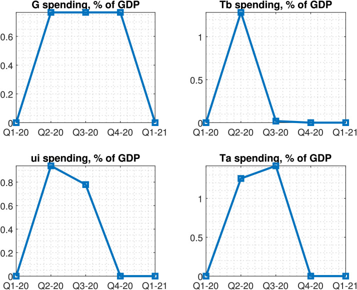
Table 2 summarizes the data for the main programs as well as to which model object they are mapped. Support to firms includes the Paycheck Protection Program, the Economic Stabilization Program, and the Air Carrier Worker Support program; all these programs were active in 2020Q2 and 2020Q3 but had mostly expired by the end of the year. Total outlays in these programs amounted to 2.6% of GDP, above the 2% that was initially prescribed. Lump-sum transfers to households $T_t^b$ were mostly sent in April and May, and so the bulk of the spending occurred in 2020Q2; total spending was 1.3% of GDP (vs initial 1.2%). Total spending in UI programs amounted to 1.7% of GDP (vs. initial 1.2%). Finally, total measured outlays for $G_t$ were about 1.1% of GDP. For this reason, for this instrument, I ignore the data and simply consider equal impulses of 2.3%/3 of GDP for the last three quarters of 2020. I do this for several reasons: first, outlays for this variable are very hard to measure accurately (at least in real time), as they include many different types of spending across many departments and programs. Second, this is the variable for which there is by far the largest discrepancy between measured outlays and those initially predicted in the CARES Act, unlike the other programs where the measured outlays roughly coincide with the initially committed amounts. Third, it is very likely that this type of spending continued through 2020Q4, for which data are not yet available. Fig. 1 plots the discretionary fiscal policy impulses that result from mapping the data in Table 2 to the model.

Table 2.

Outlays associated with programs under the CARES Act. Outlays for each quarter are expressed in % of 2019Q4 GDP ($21.4 tn). PEUC: Pandemic Emergency Unemployment Compensation, PUA: Pandemic Unemployment Assistance, PUC: Federal Pandemic Unemployment Compensation. Sources: BEA, Monthly Treasury Statement (Dept. of Treasury), Haver. N/A = data not available as of early December 2020.

Program	Model Object	2020Q1	2020Q2	2020Q3	2020Q4
Paycheck Protection Program	$T_t^a$	0.0	1.094	1.354	0.0
Economic Stabilization Program	$T_t^a$	0.0	0.053	0.039	0.0
Air Carrier Worker Support	$T_t^a$	0.0	0.108	0.026	0.0
Economic Impact Payments	$T_t^b$	0.0	1.283	0.018	0.0
Additional UI (PEUC, PUA, PUC)	${\text{ui}}_t$	0.0	0.938	0.779	N/A
State/Local Govt Relief Fund	$G_t$	0.0	0.772	0.019	N/A
Paycheck Protection Program	$G_t$	0.0	0.203	0.085	N/A

Fig. 1.

Modeling of the CARES Act: Discretionary fiscal policy impulses fed to the model, based on the measured fiscal policy response in 2.

3.3.2. Measuring the pandemic shock

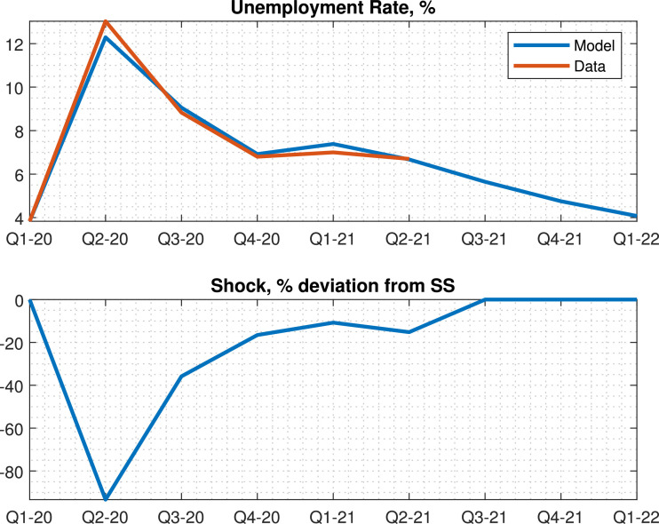
To measure the pandemic shock, I then ask the following question: what is the sequence ${\left\{{\alpha }_t\right\}}_{t=2020Q2}^{T=2021Q2}$ that allows the calibrated model to match the path of unemployment (realized and forecasted), given that the shocks in Fig. 1 are simultaneously fed to the model? Thus, the matching exercise accounts for the equilibrium effects of fiscal policy measures. As mentioned, I assume that due to the effects of the vaccine, the shock completely disappears by 2021Q3 and the economy then transitions back to normal. I assume that there is no persistence, so the shock is completely gone by that quarter. The resulting paths for unemployment and ${\alpha }_t$ are shown in Fig. 2 . By construction, the model is able to almost exactly match the data,18 hitting an unemployment rate of 13.03% in 2020Q2. This requires an extremely large negative shock of -93% to ${\alpha }_t$ in 2020Q2; the following shocks are smaller in magnitude as unemployment falls.

Fig. 2.

The top panel plots the path of unemployment in the model vs. data. Data for realized unemployment is taken from FRED (quarterly average through 2020Q3, series UNRATE), while data for projected unemployment is the median forecast in the November 2020 report of the Survey of Professional Forecasters provided by the FRB Philadelphia (for 2020Q4-2021Q2). The bottom panel plots the implied path of ${\alpha }_t$.

3.4. Pandemic experiment

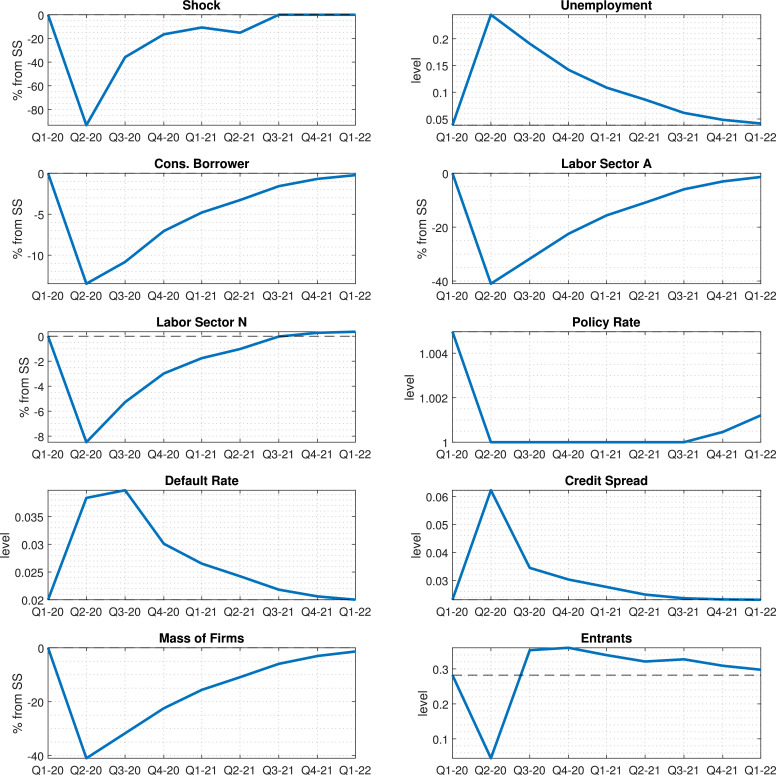
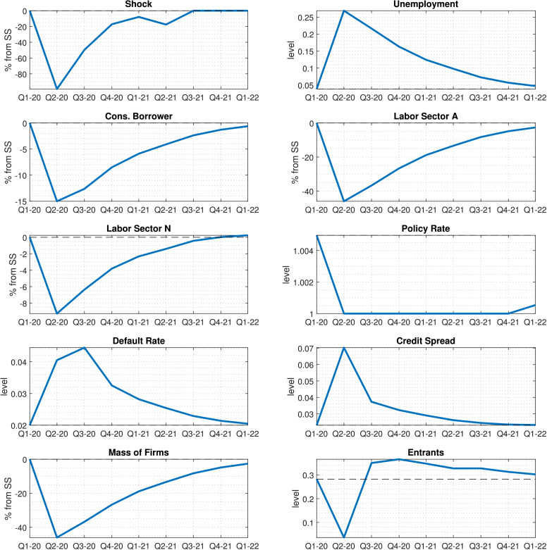
Fig. 3 plots the response of selected variables to the estimated ${\alpha }_t$ shock. The path of the shock is plotted in the first panel. The shock causes a 40% drop in employment in the services sector (fourth panel). The loss of these jobs affects borrowers, whose consumption falls by almost 15%. This drop in non-service consumption also leads to a drop in employment in the other sector, of about 8%. Combined, these drops in employment lead to a 15% contraction in GDP that lasts for the full three quarters. The sixth panel shows that this recession pushes the economy to the ZLB for the duration of the shock. The bottom two panels show that the loss in employment leads to a doubling of (quarterly) default rates. This in turn affects the capitalization of the financial sector, making lending spreads rise due to the financial constraint, which in turn further amplifies the drop in borrower consumption and rise in defaults. Persistence arises from the only slow-moving state variable, the number of firms in the affected sector. Due to entry costs, the economy takes a while to recover from the shock even if job creation becomes again positive in 2020Q3 (relative to the steady state).

Fig. 3.

Model counterfactual response to the estimated sequence of shocks ${\left\{{\widehat{\alpha }}_t\right\}}_t^T$ without fiscal policy response 2020Q1-2021Q2.

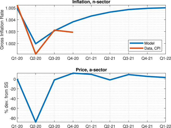
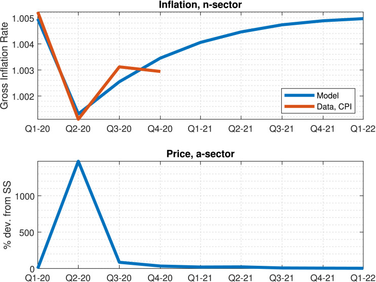
Inflation during the pandemicFig. 4 plots the response of inflation in the non-services sector ${\Pi }_t$ and of the price of services $p_t^a$ to the estimated pandemic shock. The figure shows that the pandemic causes a sustained decline in inflation in the non-services sector, which is to be expected given the behavior of employment in this sector and the presence of a New-Keynesian Phillips curve. Inflation falls to 0.8% (yearly) and then slowly recovers to its steady state level.19 In the services sector, prices are flexible, and so I plot the price of the services good in terms of the numeraire. The price of non-services falls considerably, given that demand collapses by construction and prices are perfectly flexible. As demand recovers, so does the price of the services good, whose path resembles that of the shock.

Fig. 4.

Response of ${\Pi }_t,p_t^a$ to the estimated sequence of shocks for ${\alpha }_t,$ 2020Q1-2021Q2. The CPI series is taken as the quarterly average of the year-on-year change of the CPI (FRED series CPIAUCSL).

Given the preference structure, and the fact that only savers consume services, there is no obvious ideal price index in this model. The path of inflation in the non-services sector does resemble the path of the CPI in the US but falls by slightly less than in the data. It is not clear how to interpret the path of the price of services, as this good effectively ceases to be traded. Several studies have focused on the challenges raised by the pandemic for the measurement of inflation (Cavallo, 2020, Jaravel, O’Connell, 2020).20

4. The effects of fiscal policy during the pandemic

I consider, separately, the effects of deploying the following instruments:

• 1.An increase in government consumption in $n$-sector, $G_t$.
• 2.A payroll tax cut, ${\tau }_t^l$.
• 3.An uncrease in unemployment insurance, ${\text{ui}}_t$.
• 4.Unconditional transfers to all agents, $T_t^b$.
• 5.Transfers to services sector firms, $T_t^a$.

In all cases, I consider a one-time impulse with zero persistence for each instrument. The impulse arrives at the beginning of 2020Q2, the quarter the pandemic begins. While rough, this exercise allows us to understand and isolate the different effects of these policies. In the subsequent section, I estimate the joint effects of some of these policies that were used in the CARES Act. I choose the impulses so that the resulting deficits are somewhat comparable — of similar magnitudes. I focus on packages that involve a quarterly increase in the deficit on impact of $200 billion, or roughly 3.7% of quarterly GDP. The size and intensity of the interventions certainly matter since the model features nonlinearities such as the ZLB. A deeper exploration into the ideal size of each impulse is left for further research. At the end of this section, I present tables with model-based estimates for present-value fiscal multipliers, which partly take into account the differing sizes of the interventions.

Next, I describe in more detail the effects of these policies. Many of them generate similar effects from a qualitative perspective. The quantitative effects are different, however, and I compare these effects using multipliers at the end of this section.

4.1. The effects of different policies

Government consumption of non-services This is comparable to the traditional increase in $G_t$ in one-sector New-Keynesian models. I assume that it is not feasible for the government to purchase services directly: this would be roughly equivalent to a transfer to those firms, which is considered separately.

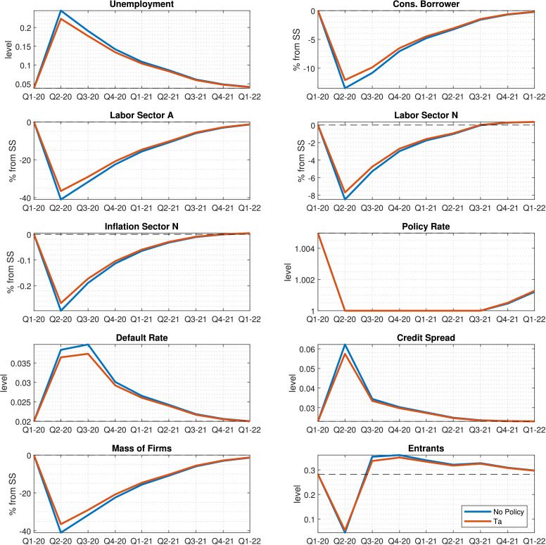
Fig. 5 plots the effects of this policy on selected variables. The blue lines correspond to the crisis absent intervention (as in Fig. 3), while the orange lines include the intervention. The key effect of the policy is seen in the fourth panel: a large increase in government consumption helps sustain employment in the non-services sector. This, in turn, somewhat moderates the drop in borrower consumption and the rise in unemployment. Finally, the fact that employment does not fall by as much also helps contain default rates and, via the banking system, credit spreads. This policy has no direct effect on the services sector; in fact, if anything, it makes conditions slightly worse by driving up wages for affected firms.

Fig. 5.

Response to a $\sim$$200 bn increase in $G_t,$ government consumption of non-service goods given estimated sequence of the pandemic shock ${\left\{\widehat{\alpha }\right\}}_t^T$.

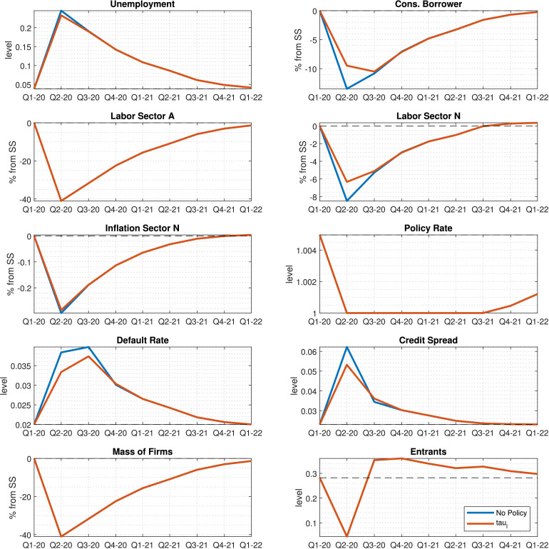
Payroll tax cuts To achieve a total deficit of the same size, the intervention consists of a one-time tax cut of 50%; i.e., the tax rate is cut by half. The effects of the tax cut, shown in Fig. 6 , look relatively similar to those shown in Fig. 5, with the main exception being that they do not stimulate labor in the non-services sector as much as the more targeted policy of government consumption. Tax cuts still help sustain borrower income, which in turn results in a slightly lower rise in unemployment and a decrease in default rates. One important thing to notice is that this model may underestimate the effectiveness of tax cuts, as discussed before: due to the assumption of labor market rationing, there are no direct benefits from removing labor market distortions.

Fig. 6.

Response to a $\sim$$200 bn payroll tax cut given estimated sequence of the pandemic shock ${\left\{\widehat{\alpha }\right\}}_t^T$.

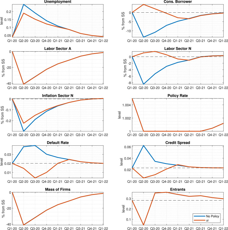
Unemployment insurance Next, we consider a one-time increase in unemployment insurance payments. To achieve a $200 bn intervention, the unemployment insurance transfer per agent is raised by 82%. As shown in Fig. 7 , the effects are noticeably larger on borrower consumption, which now increases on impact. This is somewhat predictable: payroll tax cuts benefit agents who remain employed when a large fraction of agents become unemployed. With unemployment insurance, it is the opposite: it helps unemployed agents when a large fraction of agents become unemployed. The rise in borrower consumption helps sustain demand in the non-services sector, as seen in the fifth panel. Also note that while the intervention happens only in one quarter, the effects are relatively persistent. This has to do with the fact that borrowing costs remain low, as this increase in unemployment insurance considerably lowers default rates (as unemployed agents tend to have higher default rates than employed ones), which results in an implicit recapitalization of the banking system.

Fig. 7.

Response to a $\sim$$200 bn increase in UI given estimated sequence of the pandemic shock ${\left\{\widehat{\alpha }\right\}}_t^T$.

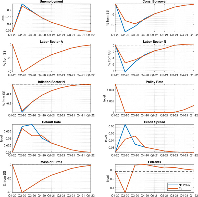
Unconditional transfersFig. 8 plots the effect of a transfer that is given to everyone in this economy, including savers. The effects are similar to those of the payroll tax cut, which is not surprising, as the incidence is effectively the same.

Fig. 8.

Response to a $\sim$$200 bn unconditional transfer given estimated sequence of the pandemic shock ${\left\{\widehat{\alpha }\right\}}_t^T$.

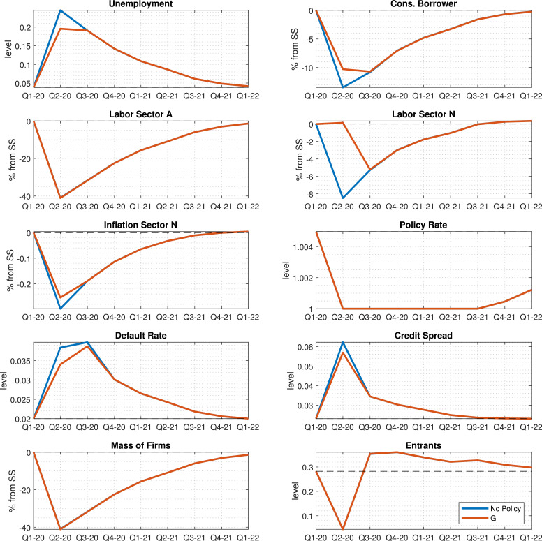
Liquidity assistance to service firmsFig. 9 shows the effects of a per-wage subsidy to firms in the services sector. Unlike other interventions, this type of intervention (i) helps mitigate the fall in employment in the services sector and (ii) has longer-lasting effects that result from a lower firm exit rate. The general equilibrium effects are reflected in borrower consumption and labor in the non-services sector. This experiment is not totally fair to this policy, to the extent that this is the only policy that explicitly targets the $a$-sector but does so for only one period, while agents expect the negative demand shock to last for an extra four periods. The remaining four periods without assistance affect the value of service firms, $V_t\left(A_t\right),$ which does not rise by as much as it would should the assistance last for the duration of the pandemic.

Fig. 9.

Response to a $\sim$$200 bn transfer to service firms given estimated sequence of the pandemic shock ${\left\{\widehat{\alpha }\right\}}_t^T$.

4.2. Fiscal multipliers

While the sizes of the interventions are calibrated to be of around $200 bn, or 3.7% of quarterly GDP, there are dynamic and general equilibrium effects that influence the path of government expenditure and revenue and that differ across instruments. One common way to control for these effects along with the size of the intervention is to compute present value discounted multipliers as in Mountford and Uhlig (2009) or Ramey (2011). For a given outcome variable of interest $x,$ the multiplier is computed as

$${\mathcal{M}}_T\left(\omega \right)=\frac{{\sum }_{t=1}^T{\prod }_{j=1}^t{R}_j^{-1}(x_t^{\text{Stimulus}}-x_t^{\text{No}\text{Stimulus}})}{{\sum }_{t=1}^T{\prod }_{j=1}^t{R}_j^{-1}({\text{Spending}}_t^{\text{Stimulus}}-{\text{Spending}}_t^{\text{No}\text{Stimulus}})}$$

The multiplier is computed for a given instrument $\omega \in \{G_t,{\tau }_t^l,{\text{ui}}_t,T_t^b,T_t^a\}$ and at a given horizon $T$. I set $T$ equal to 20 quarters: this is a typical value for the horizon, but it may underestimate the effects of some of the policies that have more persistent effects, such as liquidity assistance. Since the discount rate $R_j$ differs across the economies with policy and with no policy, it is not obvious which one to use. I use the interest rate in the no-policy economy so as to keep the comparison between different tools as fair as possible.

Table 3 compares multipliers for a variety of variables: total employment, income net of government transfers, borrower consumption, saver consumption of non-service goods, and GDP. Income net of transfers is essentially income for the borrowers and is defined as21

$${\text{Income}}_t=(1-{\tau }_t^l)w_t(N_t^a+N_t^n)+(1-N_t^n-N_t^a){\text{ui}}_t+T_t^b$$

Table 3.

Fiscal multipliers.

Instrument	Description	${\mathcal{M}}_{20}\left(\omega \right),$ Employment	${\mathcal{M}}_{20}\left(\omega \right),$ Income	${\mathcal{M}}_{20}\left(\omega \right),$$C_t^b$	${\mathcal{M}}_{20}\left(\omega \right),$$C_t^s$	${\mathcal{M}}_{20}\left(\omega \right),$ GDP
$G$	Govt. Consumption	1.2228	0.5687	0.5311	0.0087	1.2548
${\tau }_t^l$	Payroll Tax	0.5914	1.3513	1.2853	0.0146	0.6058
$\varsigma$	UI	0.6539	1.4824	1.4140	0.0165	0.6660
$T_t^b$	Uncond. Transfer	0.5542	1.2574	1.2049	0.0135	0.5675
$T_t^a$	Liquidity Assist.	2.5136	1.1740	1.1526	$-$0.0408	0.4497

In terms of income, the largest multipliers are generated by UI. Payroll tax cuts and unconditional transfers are also effective but generate lower multipliers, as they are less well-targeted to agents with lower incomes. UI is, furthermore, very well targeted in terms of its timing, as these transfers arrive precisely at a time when unemployment surges. Multipliers on borrower consumption are very similar to those of income, which is to be expected since borrowers are constrained and therefore have a high marginal propensity to consume out of their current income. Any differences reflect changes in the cost of credit from banks.

Multipliers on saver consumption are very low. Savers react relatively little to fiscal policy, as they are unconstrained. Savers are “Ricardian” in the sense that they purchase public debt and pay lump-sum taxes and, therefore, react to changes in the present value of government liabilities. Note however that the general-equilibrium effects are strong enough to offset the usual fall in consumption for savers.

Employment multipliers are particularly high for liquidity assistance. This is mostly due to the long-lasting effects of this policy. While its effects on impact are smaller than those of other policies, liquidity assistance prevents firm exit and ensures a faster recovery.

GDP multipliers are reported in the last column. As argued before, it is not clear whether adopting measures that stabilize GDP is appropriate in this situation. Still, I report the multipliers for completeness. The measure that yields the largest GDP multiplier is government consumption. It is well known that it is “hard to beat” government consumption in this class of models (Oh and Reis, 2012), especially in the absence of very strong links between the balance sheets of households and the financial system. Payroll tax cuts, increases in UI, and unconditional transfers all deliver somewhat similar results. UI performs the best, as it is the most well-targeted, while unconditional transfers perform the worst of those three, as they are the least well-targeted.

Literature on fiscal multipliers during COVID-19 It is also worth comparing some of these results to other studies on the relative effectiveness of fiscal policies during COVID-19. As mentioned in the introduction, Bayer et al. (2020) study the relative effectiveness of UI/conditional transfers vs. lump-sum/unconditional transfers in a much richer model of household heterogeneity. Their richer setup, which includes idiosyncratic income and unemployment risk, leads them to find much larger differences in terms of the relative effectiveness of the two policies. My setup is simpler than theirs when it comes to modeling the income and wealth distribution of households, as this allows me to also study other types of fiscal policies, but I show that the qualitative result still holds even in the absence of that detail in terms of modeling heterogeneity. Importantly, and as I show in the following section, this ranking of the policies inverts during normal times. My results also differ than those of Guerrieri et al. (2020), who show that traditional government spending may have a very muted effect in an economy under lockdown. This difference is related to different assumptions regarding labor mobility. In that paper, the authors assume that a certain group of constrained households only work in the sector that is shut down. Thus government spending in that sector cannot possibly raise their income. In contrast, my model features both households working in both sectors, which allows the government to raise income for constrained households by spending in the non-shutdown sector.

4.3. Dissecting the effect on borrower income

The change in borrower income on impact is shown in Fig. 10 . This figure confirms that UI increases have the largest effect. Note that in this and the subsequent figures we are comparing % changes for a given impulse and not adjusting for dollars spent as in the previous paragraphs. Transfers generate better results than payroll tax cuts. It all boils down to how well targeted a policy is.

Fig. 10.

% change in income due to policy, on impact, given estimated sequence of the pandemic shock ${\left\{\widehat{\alpha }\right\}}_t^T$.

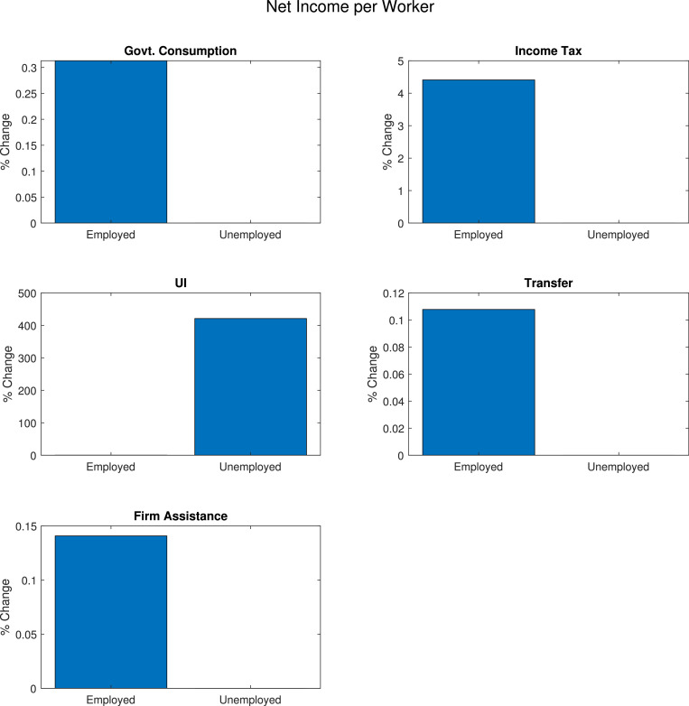
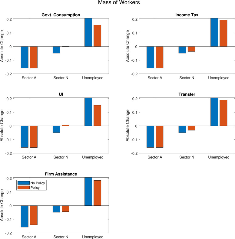
Figs. 11 and 12 help us understand how well/poorly targeted each type of policy is, by decomposing the effect of each policy on prices and quantities (on impact). Fig. 11 plots net income per worker (employed or unemployed) across policies. It shows, for example, that payroll tax cuts raise incomes for employed workers exclusively, while UI raises incomes for unemployed workers almost exclusively (there is a small increase in employed income that is not visible due to the scale). Transfers and government consumption of non-services operate via traditional aggregate demand effects, thus raising demand for $n$-sector goods and therefore earnings in this sector, but they have no effect on other types of workers. Finally, liquidity assistance to $a$-sector firms helps sustain wages in this sector somewhat. Fig. 12 plots absolute changes in the number of workers in each sector, in the baseline economy with no policy (blue bars) and in the economy with the policy impulse (orange bars).22 While there are minor variations across policies, the overall patterns are the same: the shock leads to a large reduction in $a$-sector employment, a moderate reduction in $n$-sector employment, and a large increase in unemployment. Figs. 11 and 12 combined show very clearly why UI is the superior policy to stabilize household income, as they target the category of households that increases the most due to the shock.

Fig. 11.

% change on net income per worker due to policy, across sectors, given estimated sequence of the pandemic shock ${\left\{\widehat{\alpha }\right\}}_t^T$. Note that each panel has a different scale.

Fig. 12.

Total change in workers, across sectors, given estimated sequence of the pandemic shock ${\left\{\widehat{\alpha }\right\}}_t^T$.

4.4. State dependence and model fit

Model fit: multipliers in normal times In order to assess the fit of the model and to argue that the calibration generates plausible results, I recompute fiscal multipliers for the same policy instruments but in the absence of the pandemic shock. Thus, I use the calibrated model to compute fiscal multipliers in “normal times,” where there are no other shocks besides the stimulus and the baseline no-stimulus economy is simply its steady state. These results are reported in Table 4 . The GDP and employment multipliers of government consumption are 0.81 and 0.85, respectively, well within the range of values that have been estimated in the literature for the effects of government purchases in the US (Auerbach, Gorodnichenko, 2012, Ramey, Zubairy, 2018). The multipliers for tax and transfer policies are low, between 0.34 and 0.39. These multipliers are low and in line with the values estimated by event studies for tax rebates in the US.23 This, again, is consistent with the well-known finding that these policies tend to be inferior to direct government purchases in terms of employment stimulus. These results suggest that the model structure and calibration are able to generate plausible results that are consistent with the literature.

Table 4.

Fiscal multipliers: No pandemic shock.

Instrument	Description	${\mathcal{M}}_{20}\left(\omega \right),$ Employment	${\mathcal{M}}_{20}\left(\omega \right),$ Income	${\mathcal{M}}_{20}\left(\omega \right),$$C_t^b$	${\mathcal{M}}_{20}\left(\omega \right),$$C_t^s$	${\mathcal{M}}_{20}\left(\omega \right),$ GDP
$G$	Govt. Consumption	0.8468	0.4005	0.2714	$-$0.1561	0.8054
${\tau }_t^l$	payroll tax	0.3982	1.2406	1.1281	$-$0.0634	0.3792
$\varsigma$	UI	0.3612	1.2686	1.0891	$-$0.0718	0.3445
$T_t^b$	Uncond. Transfer	0.3815	1.1805	1.0769	$-$0.0599	0.3633
$T_t^a$	Liquidity Assist.	0.3197	0.1512	0.0462	$-$0.0750	$-$0.1091

Nonlinearities and state dependence These results also highlight that the model is highly nonlinear and features a nontrivial amount of state dependence. First, the multipliers in normal times are much lower than those during the pandemic. This is true for all fiscal policy instruments, but it is particularly striking for liquidity assistance to firms: the employment multipliers are very small during normal times (0.32 vs. 2.51 in the pandemic), and the GDP multipliers are even negative ($-$0.11 vs. 0.45). Liquidity assistance is therefore a very bad policy during normal times, but it has a very stabilizing effect on employment in the face of a pandemic shock. Second, the ranking of multipliers for employment changes between normal times and the pandemic. As shown in the previous subsections, UI dominates tax cuts or lump-sum transfers during the pandemic, but UI itself is dominated by either of these policies during normal times. While the ranking of these policies over borrower income is the same, the effects arise mostly due to the fact that UI has the most negative effect on saver consumption, as it is the closest thing to a direct transfer from savers to borrowers in this model.

5. The effects of the CARES act of 2020

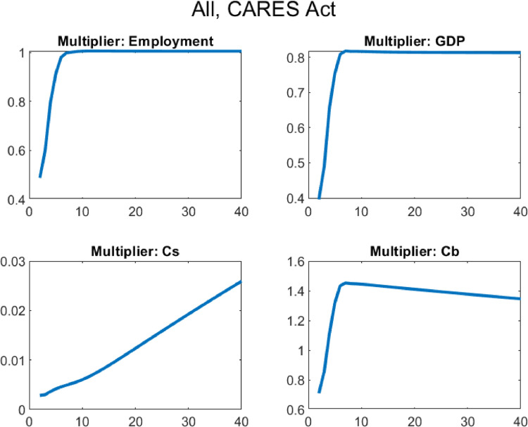
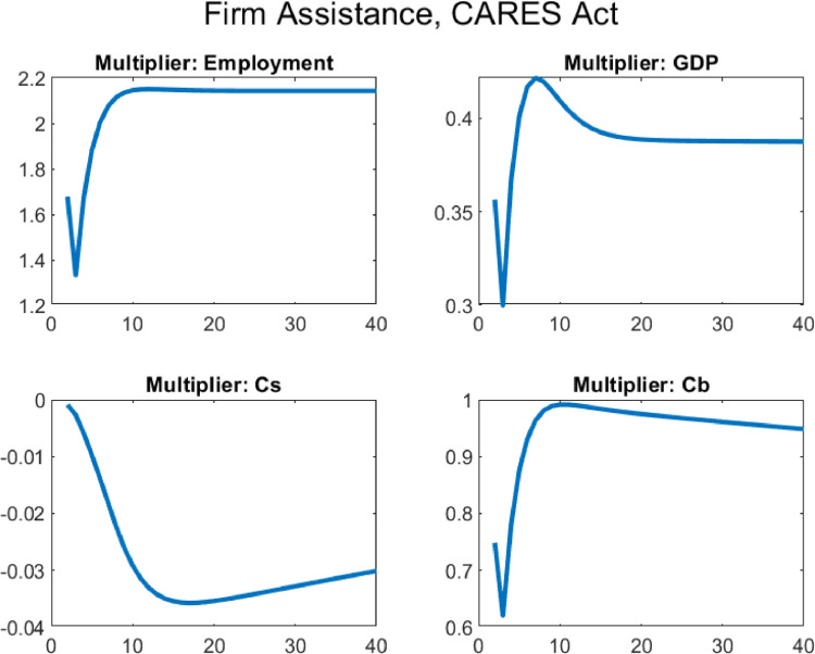
Finally, I use the model and the estimated fiscal impulses and pandemic shock to quantitatively evaluate the CARES Act of 2020. I compute the fiscal multipliers for the sequences plotted in Fig. 1, both one by one and for the aggregate package. The results are shown in Table 5 . The fiscal package as a whole has an income multiplier of 1.47 and an employment multiplier of slightly over 1. The following rows decompose the multiplier across different policies. These numbers are obtained by considering one policy at a time, similar to the exercise in previous sections. Even though the interventions have different sizes and lengths, the results from the baseline exercise are virtually unchanged, with UI and transfer payments providing most of the income and consumption stabilization, and liquidity assistance to firms providing most of the employment stabilization due to its long-run effects.24

Table 5.

Aggregate multipliers for the CARES Act of 2020 and decomposition.

Instrument	Description	${\mathcal{M}}_{20}\left(\omega \right),$ Employment	${\mathcal{M}}_{20}\left(\omega \right),$ Income	${\mathcal{M}}_{20}\left(\omega \right),$$C_t^b$	${\mathcal{M}}_{20}\left(\omega \right),$$C_t^s$	${\mathcal{M}}_{20}\left(\omega \right),$ GDP
All Policies		1.0066	1.4712	1.4097	0.0124	0.8142
$G$	Govt. Consumption	1.2396	0.5788	0.5472	0.0110	1.2633
$\varsigma$	UI	0.6630	1.4900	1.4270	0.0176	0.6732
$T_t^b$	Uncond. Transfer	0.5533	1.2570	1.2029	0.0135	0.5666
$T_t^a$	Liquidity Assist.	2.1438	1.0021	0.9749	$-$0.0354	0.3887

6. Conclusion

In the context of a calibrated DSGE model that matches the path of the US unemployment rate in 2020, I find that the most effective tool to stabilize household income and borrower consumption in the context of an exogenous shock that leads to the shut down of the services sector is an increase in UI benefits. Overall, programs that involve transfers of some kind to households seem to be effective, with UI being the best targeted. Unconditional transfers are likely to be less costly in terms of implementation and deliver somewhat similar (but weaker) results. Firm liquidity assistance programs are effective at maintaining employment overall and have longer-lasting effects. I show that the effects of fiscal policy in this model are extremely state-dependent, and the ranking of policies changes significantly with and without the pandemic shock.

The analysis in this paper has many caveats and abstracts from many important considerations. It abstracts from several important aspects of fiscal policy analysis, such as the sizes of the interventions (Brinca et al., 2019) and potential complementarities and substitutabilities between policies (Faria-e-Castro, 2018). The current analysis also abstracts from endogenous labor supply decisions, which can be important to analyze the medium-run effects of policies such as tax cuts and UI. However, the existing literature suggests that these incentive problems played a limited role in the context of the CARES Act. Finally, it completely abstracts from the possibility that fiscal policy can be deployed to reduce the duration and intensity of the shock caused by the pandemic, and it also abstracts from the fact that stimulating economic activity may actually be detrimental in fighting the pandemic.

There are also other important caveats that were not previously discussed. There are implementation lags that can be made worse by attempts to better target policies. Better targeted policies may additionally entail extra costs associated with bureaucracy. It may sometimes be better to undertake a slightly worse policy whose implementation requires less information and time, i.e., unconditional transfers vs. expansion of unemployment insurance eligibility. Also, I completely abstract from other potential policies that have been part of the debate: the role of state fiscal policy, health insurance, debt forgiveness and restructuring, moratoria on debt (and bill) repayments, etc. For a detailed discussion of some of these policies, see Dupor (2020).

Appendix A. Full list of equilibrium conditions

Borrowers (${\lambda }_t$ is the Lagrange multiplier on the borrowing constraint):

$$\begin{array}{cc}& {\epsilon }_t^e=\frac{B_{t-1}^b}{\chi {\Pi }_t}-w_t(1-{\tau }_t^l)\hfill \\ & {\epsilon }_t^u=\frac{B_{t-1}^b}{\chi {\Pi }_t}-{\text{ui}}_t\hfill \\ & F_t^b=(N_t^a+N_t^n)F^e\left({\epsilon }_t^e\right)+(1-N_t^a-N_t^n)F^u\left({\epsilon }_t^u\right)\hfill \\ & m_{t+1}^b\equiv {\beta }^b\frac{u^{\prime }\left(C_{t+1}^b\right)}{u^{\prime }(C_t^{)}b}\hfill \\ & Q_t^b-{\lambda }_t={\mathbb{E}}_t\frac{m_{t+1}^b}{{\Pi }_{t+1}}(1-F_{t+1}^b)\hfill \\ & C_t^b+\frac{B_{t-1}}{\chi {\Pi }_t}(1-F_t^b)\le (N_t^a+N_t^n)w_t(1-{\tau }_l)+(1-N_t^a-N_t^n){\text{ui}}_t+Q_t^b{B}_t^b/\chi +T_t^b-T_t^s\hfill \\ & Q_t^b{B}_t^b\chi \le \Gamma \perp {\lambda }_t\ge 0\hfill \end{array}$$

Banks (${\mu }_t$ is the Lagrange multiplier on the leverage constraint):

$$\begin{array}{cc}& {\mathbb{E}}_t\frac{m_{t+1}^s}{{\Pi }_{t+1}}(1-\theta +\theta {\Phi }_{t+1})[\frac{1-F_{t+1}^b}{Q_t^b}-\frac{1}{Q_t}]={\mu }_t\kappa \hfill \\ & {\mathbb{E}}_t\frac{m_{t+1}^s}{{\Pi }_{t+1}}(1-\theta +\theta {\Phi }_{t+1})={\Phi }_t(1-{\mu }_t)Q_t\hfill \\ & Q_t^b{B}_t^b=E_t+Q_t^d{D}_t\hfill \\ & \kappa Q_t^b{B}_t^b\le {\Phi }_t{E}_t\perp {\mu }_t\ge 0\hfill \\ & E_t={\Pi }_t^{-1}\theta ((1-F_t^b)B_{t-1}^b-D_{t-1})+\varpi \hfill \end{array}$$

Savers:

$$\begin{array}{cc}& m_{t+1}^s\equiv {\beta }^s\frac{u^{\prime }\left(C_{t+1}^s\right)}{u^{\prime }\left(C_t^s\right)}\hfill \\ & Q_t={\mathbb{E}}_t\frac{m_{t+1}^s}{{\Pi }_{t+1}}\hfill \\ & C_t^a={\left[{\alpha }_t\frac{1}{p_t^a{u}^{\prime }\left(C_t^s\right)}\right]}^{1/{\sigma }_a}\hfill \end{array}$$

Non-services sector:

$$\begin{array}{cc}& \eta \frac{{\Pi }_t}{\Pi }(\frac{{\Pi }_t}{\Pi }-1)+ϵ[\frac{ϵ-1}{ϵ}-\frac{w_t}{A_t}]=\eta {\mathbb{E}}_t{m}_{t+1}^s\frac{Y_{t+1}^n}{Y_t^n}\frac{{\Pi }_{t+1}}{\Pi }(\frac{{\Pi }_{t+1}}{\Pi }-1)\hfill \\ & Y_t^n=A_t{N}_t^n[1-0.5\eta {(\frac{{\Pi }_t}{\Pi }-1)}^2]\hfill \\ & C_t=C_t^s+C_t^b\hfill \\ & C_t+G_t+\Psi \left({\overline{c}}_t\right)J_{t-1}=Y_t^n\hfill \\ & w_t=\xi A_t{(N_t^n+N_t^a)}^{\zeta }\hfill \end{array}$$

Services sector:

$$\begin{array}{cc}& {\overline{c}}_t=A_t{p}_t^a-w_t+w_t{T}_t^a+{\mathbb{E}}_t{m}_{t+}^s[H_{t+1}^a{\overline{c}}_{t+1}-\Psi \left[{\overline{c}}_{t+1}\right]]\hfill \\ & N_t^a=J_t\hfill \\ & J_t=H_t^a{J}_{t-1}+{\nu }_t\hfill \\ & {\overline{c}}_t\le \kappa {\nu }_t^{\psi }\perp {\nu }_t\ge 0\hfill \\ & H_t^a={\int }_0^{{\overline{c}}_t}\mathrm{d}H\left(c\right)\hfill \\ & \Psi \left[{\overline{c}}_t\right]={\int }_0^{{\overline{c}}_t}c\mathrm{d}H\left(c\right)\hfill \\ & (1-\chi )C_t^a=A_t{N}_t^a\hfill \end{array}$$

Government and central bank:

$$\begin{array}{cc}& G_t+\frac{B_{t-1}^g}{{\Pi }_t}+(1-N_t^a-N_t^n){\text{ui}}_t+T_t^b+T_t^a{w}_t{H}_t^a\hfill \\ \hfill =& {\tau }^l{w}_t(N_t^n+N_t^a)+{\tau }^k[Y_t^n(1-d_t)-w_t{N}_t^n+(p_t^a-w_t)N_t^a-\Psi \left({\overline{c}}_t\right)J_{t-1}]+Q_t{B}_t^g+T_t^s\hfill \\ & T_t^s={\left(\frac{B_{t-1}^g}{{\overline{B}}^g}\right)}^{{\varphi }_{\tau }}-1\hfill \\ & \frac{1}{Q_t}=\max \{1,{\left(\frac{{\Pi }_t}{\overline{\Pi }}\right)}^{{\varphi }_{\Pi }}{\left(\frac{p_t^a}{p_{t-1}^a}\right)}^{{\varphi }_a}{\left(\frac{1-N_t^a-N_t^n}{\overline{u}}\right)}^{{\varphi }_{GDP}}\}\hfill \\ & GD{P}_t=Y_t^n+p_t^a{Y}_t^a\hfill \end{array}$$

Appendix B. Keynesian supply shocks

In a recent paper, Guerrieri et al. (2020) show that, under certain conditions, supply shocks can generate demand-like effects in models with incomplete markets, multiple sectors, and nominal rigidities. In particular, they show that depending on the values for the elasticity of intertemporal substitution and for the elasticity of substitution between goods produced in two different sectors, negative supply shocks in one sector can lead to a fall in output and the real interest rate. These are labeled “Keynesian supply shocks.” Additionally, recent empirical work has argued that the pandemic shock and subsequent containment measures combine aspects of demand and supply shocks (Brinca et al., 2020).

In this section, I show that the current model can also generate Keynesian supply shocks for certain parametrizations. Recall that the demand for services by savers is given by

$$C_t^a={\left[\frac{{\alpha }_t}{p_t^a}{\left(C_t^s\right)}^{\sigma }\right]}^{1/{\sigma }_a}$$

and we can derive the elasticity of substitution between services and non-services as

$$-\frac{d\log (C_t^a/C_t^s)}{d\log p_t^a}=\frac{1}{{\sigma }_a}$$

The model can generate Keynesian supply shocks as long as the elasticity of substitution is high enough:

$$\frac{1}{{\sigma }_a}>1$$

This condition is similar to $1/\rho >1$ in Guerrieri et al. (2020). Fig. 13 shows what a Keynesian supply shock looks like in this model. I set ${\sigma }_a=0.5$ and introduce a new shock $z_t,$ which reduces the productivity of the services sector. Given that labor is demand-determined in this model, this approach is very similar to an exogenous reduction of labor supply as considered by Guerrieri et al. (2020). I estimate a sequence of shocks to $z_t$ using the same procedure as in the main text — so that the model can match the path of the unemployment rate given the observed paths for fiscal policy outlays. The figure shows that the main dynamics of the pandemic scenario are unchanged, with a large drop in the consumption and production of both types of goods.25

Fig. 13.

Pandemic as a Keynesian Supply Shock.

Tables 6 and 7 present the fiscal multipliers for the baseline set of policies and for the CARES Act, respectively, when the pandemic is modeled as a supply shock. Most of the results are unchanged with one exception: liquidity assistance to firms is now considerably more effective, especially in terms of sustaining borrower income. My results regarding the effectiveness of $G$ differ from those in Guerrieri et al. (2020) due to different assumptions regarding labor mobility. In their paper, constrained households work in the shutdown sector, and so there is no way for the government to raise their income by spending. In contrast, both households, constrained and non-constrained, work in the non-shutdown sector in my model. Thus, the government can stabilize the income of borrowers by spending in the non-shutdown sector.

Table 6.

Fiscal multipliers, pandemic as a Keynesian supply shock.

Instrument	Description	${\mathcal{M}}_{20}\left(\omega \right),$ Employment	${\mathcal{M}}_{20}\left(\omega \right),$ Income	${\mathcal{M}}_{20}\left(\omega \right),$$C_t^b$	${\mathcal{M}}_{20}\left(\omega \right),$$C_t^s$	${\mathcal{M}}_{20}\left(\omega \right),$ GDP
$G$	Govt. Consumption	1.1902	0.5520	0.5146	0.0065	1.2288
${\tau }_t^l$	Income Tax	0.5751	1.3408	1.2772	0.0092	0.5923
$\varsigma$	UI	0.6387	1.4705	1.4039	0.0108	0.6526
$T_t^b$	Uncond. Transfer	0.5401	1.2502	1.1995	0.0086	0.5560
$T_t^a$	Liquidity Assist.	4.4210	2.0639	2.0873	$-$0.1610	1.8715

Table 7.

Aggregate multipliers for the CARES Act of 2020 and decomposition, pandemic as a Keynesian supply shock.

Instrument	Description	${\mathcal{M}}_{20}\left(\omega \right),$ Employment	${\mathcal{M}}_{20}\left(\omega \right),$ Income	${\mathcal{M}}_{20}\left(\omega \right),$$C_t^b$	${\mathcal{M}}_{20}\left(\omega \right),$$C_t^s$	${\mathcal{M}}_{20}\left(\omega \right),$ GDP
All Policies		1.1832	1.6140	1.5547	-0.0031	0.9651
$G$	Govt. Consumption	1.2146	0.5658	0.5344	0.0088	1.2427
$\varsigma$	UI	0.8308	1.6136	1.5527	0.0056	0.8007
$T_t^b$	Uncond. Transfer	0.5397	1.2500	1.1985	0.0086	0.5556
$T_t^a$	Liquidity Assist.	3.7373	1.7465	1.7566	$-$0.1418	1.6141

Inflation dynamicsFig. 14 replicates Fig. 4 under the assumption of Keynesian Supply Shocks, showing that the overall effect on inflation for the non-affected sector is robust to changing the nature of the underlying shock. Naturally, we now get the opposite prediction for the price of the affected sector: as demand is constant and production becomes less efficient, the price shoots up. The important result that I want to highlight is that the overall predictions regarding unemployment and the effects of policy of the model are robust to the exact underlying nature of the shock. What is important for most of the results is that the model structure (and calibration) be such that the underlying shock produces a demand recession in the non-affected sector.

Fig. 14.

Response of ${\Pi }_t,p_t^a$ to the estimated sequence of shocks for ${\alpha }_t,$ 2020Q1-2021Q2, under Keynesian Supply Shocks The CPI series is taken as the quarterly average of the year-on-year change on the CPI (FRED series CPIAUCSL).

Appendix C. Borrowers consume service goods

In the baseline version of the model, borrowers do not consume service goods. I make this modeling decision for several reasons, technical and conceptual: (i) it is documented that lower-income households tend to have a lower fraction of expenditures in services and nontradables (Boppart, 2014, Carroll, Hur, 2020); (ii) even for low values of ${\sigma }_a$ it is very hard to prevent borrowers from switching expenditure from services to non-services when faced with a utility shock, thus causing a boom in the non-services sector, which is at odds with the data. Nevertheless, I repeat the baseline exercise for a version of the model where both agents consume both goods, setting ${\sigma }_a=0.25,$ and show that the results do not change substantially. Tables 8 and 9 report the results.

Table 8.

Fiscal multipliers given a pandemic shock, both households consume services.

Instrument	Description	${\mathcal{M}}_{20}\left(\omega \right),$ Employment	${\mathcal{M}}_{20}\left(\omega \right),$ Income	${\mathcal{M}}_{20}\left(\omega \right),$$C_t^b$	${\mathcal{M}}_{20}\left(\omega \right),$$C_t^s$	${\mathcal{M}}_{20}\left(\omega \right),$ GDP
$G$	Govt. Consumption	1.1525	0.5414	0.4836	$-$0.0800	1.1755
${\tau }_t^l$	Income Tax	0.4470	1.2691	1.1743	$-$0.1892	0.4296
$\varsigma$	UI	0.4550	1.3375	1.1356	$-$0.1480	0.4347
$T_t^b$	Uncond. Transfer	0.4210	1.1983	1.1277	$-$0.1945	0.4055
$T_t^a$	Liquidity Assist.	2.0317	0.9556	0.9064	$-$0.3483	0.2237

Table 9.

Aggregate multipliers for the CARES Act of 2020 and decomposition, both households consume services.

Instrument	Description	${\mathcal{M}}_{20}\left(\omega \right),$ Employment	${\mathcal{M}}_{20}\left(\omega \right),$ Income	${\mathcal{M}}_{20}\left(\omega \right),$$C_t^b$	${\mathcal{M}}_{20}\left(\omega \right),$$C_t^s$	${\mathcal{M}}_{20}\left(\omega \right),$ GDP
All Policies		0.9574	1.2840	1.1858	$-$0.2500	0.6410
$G$	Govt. Consumption	1.1846	0.5570	0.5150	$-$0.0709	1.1945
$\varsigma$	UI	0.4547	1.3374	1.2278	$-$0.2171	0.4385
$T_t^b$	Uncond. Transfer	0.4252	1.2003	1.1292	$-$0.1891	0.4091
$T_t^a$	Liquidity Assist.	1.8440	0.8673	0.8177	$-$0.3246	0.2065

Appendix D. Multipliers at different horizons

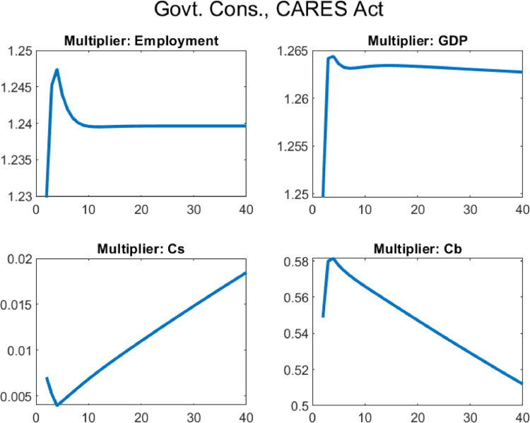
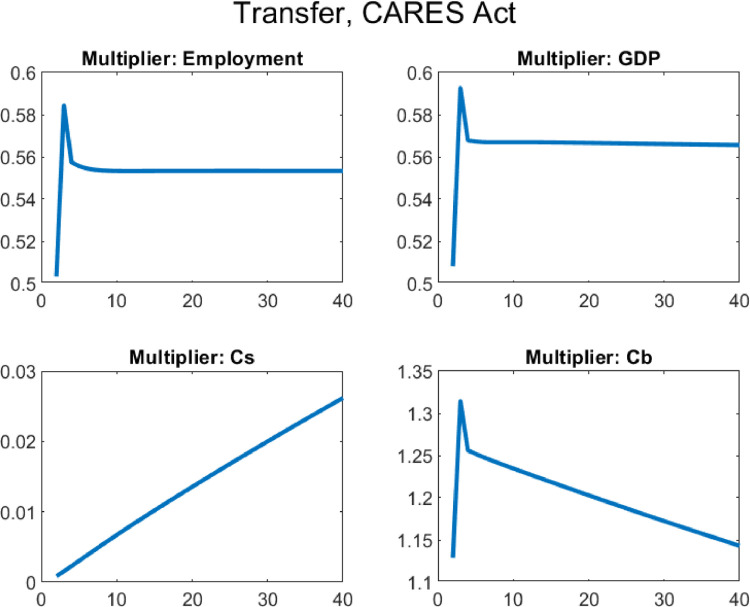
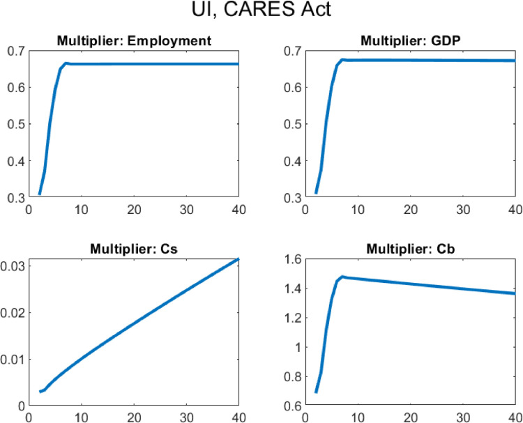
In this section, in Figs. 15 -19 , I extend the analysis in Section 4.2 and plot the multipliers for the different policies in the CARES Act at different horizons and for different outcome variables.

Fig. 16.

Multipliers of the CARES Act at different horizons: govt. spending

Fig. 17.

Multipliers of the CARES Act at different horizons: transfer

Fig. 18.

Multipliers of the CARES Act at different horizons: UI

Fig. 15.

Multipliers of the CARES Act at different horizons: all Policies

Fig. 19.

Multipliers of the CARES Act at different horizons: liquidity assistance

References

- Adjemian S., Bastani H., Juillard M., Karamé F., Maih J., Mihoubi F., Perendia G., Pfeifer J., Ratto M., Villemot S. Dynare Working Papers. CEPREMAP; 2011. Dynare: Reference Manual Version 4. [Google Scholar]
- Altonji, J., Contractor, Z., Finamor, L., Haygood, R., Lindenlaub, I., Meghir, C., O’Dea, C., Scott, D., Wang, L., Washington, E., 2020. Employment effects of unemployment insurance generosity during the pandemic. Unpublished, Tobin Center for Economic Policy at Yale University.
- Auerbach A.J., Gorodnichenko Y. Measuring the output responses to fiscal policy. Am. Econ. J.: Econ. Policy. 2012;4(2):1–27. [Google Scholar]
- Baron M. Countercyclical bank equity issuance. Rev. Financ. Stud. 2020;33(9):4186–4230. doi: 10.1093/rfs/hhaa008. [DOI] [Google Scholar]; https://academic.oup.com/rfs/article-pdf/33/9/4186/33677973/hhaa008.pdf.
- Barro R.J., Ursua J.F., Weng J. Working Paper. National Bureau of Economic Research; 2020. The Coronavirus and the Great Influenza Pandemic: Lessons from the “Spanish Flu” for the Coronavirus’s Potential Effects on Mortality and Economic Activity. [DOI] [Google Scholar]
- Bartik A.W., Bertrand M., Lin F., Rothstein J., Unrath M. Working Paper. National Bureau of Economic Research; 2020. Measuring the labor market at the onset of the COVID-19 crisis. [DOI] [Google Scholar]
- Bayer C., Born B., Luetticke R., Mueller G. CEPR Working Paper. CEPR; 2020. The Coronavirus Stimulus Package: How Large is the Transfer Multiplier? [Google Scholar]
- Berentsen A., Waller C. Optimal stabilization policy with search externalities. Macroecon. Dyn. 2015;19(3):669–700. [Google Scholar]
- Blanchard O., Galí J. Labor markets and monetary policy: a new keynesian model with unemployment. Am. Econ. J.: Macroecon. 2010;2(2):1–30. doi: 10.1257/mac.2.2.1. [DOI] [Google Scholar]
- Boar C., Mongey S. Working Paper. National Bureau of Economic Research; 2020. Dynamic Trade-offs and Labor Supply Under the CARES Act. [DOI] [Google Scholar]
- Boppart T. Structural change and the Kaldor facts in a growth model with relative price effects and non-Gorman preferences. Econometrica. 2014;82:2167–2196. [Google Scholar]
- Brinca P., Duarte J.B., Faria-e-Castro M. Working Paper. Federal Reserve Bank of St. Louis; 2020. Measuring Labor Supply and Demand Shocks during COVID-19. [DOI] [PMC free article] [PubMed] [Google Scholar]
- Brinca P., Faria-e-Castro M., Ferreira M.H., Holter H. Working Paper. Federal Reserve Bank of St. Louis; 2019. The Nonlinear Effects of Fiscal Policy. [DOI] [Google Scholar]
- Carroll D.R., Hur S. On the heterogeneous welfare gains and losses from trade. J. Monet. Econ. 2020;109(C):1–16. doi: 10.1016/j.jmoneco.2019.10. [DOI] [Google Scholar]
- Cavallo A. Working Paper. National Bureau of Economic Research; 2020. Inflation with Covid Consumption Baskets. [DOI] [Google Scholar]
- Christiano L.J., Eichenbaum M.S., Trabandt M. Unemployment and business cycles. Econometrica. 2016;84:1523–1569. [Google Scholar]
- Damodaran, A., 2020. Margins by sector for the United States. Personal Website.
- Drautzburg T., Uhlig H. Fiscal stimulus and distortionary taxation. Rev. Econ. Dyn. 2015;18(4):894–920. [Google Scholar]
- Dube, A., 2020. The impact of the federal pandemic unemployment compensation on employment: evidence from the household pule survey. Unpublished, University of Massachusetts, Amherst.
- Dupor B. Possible fiscal policies for rare, unanticipated, and severe viral outbreaks. Econ. Synop. 2020;(6):1–2. [Google Scholar]; Federal Reserve Bank of St. Louis
- Eichenbaum M., Rebelo S., Trabandt M. CEPR Discussion Papers. C.E.P.R. Discussion Papers; 2020. Epidemics in the Neoclassical and New-Keynesian Models. [Google Scholar]
- Eichenbaum M.S., Rebelo S., Trabandt M. Working Paper. National Bureau of Economic Research; 2020. The Macroeconomics of Epidemics. [DOI] [Google Scholar]
- Elenev V., Landvoigt T., van Nieuwerburgh S. CEPR Discussion Paper. CEPR; 2020. Can the Covid Bailouts Save the Economy? [Google Scholar]
- Faria-e-Castro M. Working Paper. Federal Reserve Bank of St. Louis; 2018. Fiscal Multipliers and Financial Crises. [DOI] [Google Scholar]
- Fornaro, L., Wolf, M., 2020. Covid-19 coronavirus and macroeconomic policy:some analytical notes. CREI/UPF and University of Vienna.
- Gascon, C., 2020. Covid-19: Which workers face the highest unemployment risk?On the Economy Blog, Federal Reserve Bank of St. Louis.
- Gertler M., Karadi P. A model of unconventional monetary policy. J. Monet. Econ. 2011;58(1):17–34. [Google Scholar]
- Glover A., Heathcote J., Krueger D., Ríos-Rull J.-V. Working Paper. National Bureau of Economic Research; 2020. Health versus Wealth: On the Distributional Effects of Controlling a Pandemic. [DOI] [Google Scholar]
- Guerrieri V., Lorenzoni G., Straub L., Werning I. NBER Working Paper. National Bureau of Economic Research; 2020. Macroeconomic Implications of COVID-19: Can Negative Supply Shocks Cause Demand Shortages? [Google Scholar]
- Jaravel X., O’Connell M. Real-time price indices: Inflation spike and falling product variety during the Great Lockdown. J. Publ. Econ. 2020;191(C) doi: 10.1016/j.jpubeco.2020.10. [DOI] [PMC free article] [PubMed] [Google Scholar]
- Leeper E.M., Plante M., Traum N. Dynamics of fiscal financing in the United States. J. Econometr. 2010;156(2):304–321. [Google Scholar]
- Leibovici, F., Santacreu, A. M., Famiglietti, M., 2020. Social distancing and contact-intensive occupations. On the Economy Blog, Federal Reserve Bank of St. Louis.
- McKay A., Reis R. Optimal automatic stabilizers. Rev. Econ. Stud. 2020;(Forthcoming) [Google Scholar]
- Mountford A., Uhlig H. What are the effects of fiscal policy shocks? J. Appl. Econom. 2009;24(6):960–992. doi: 10.1002/jae.1079. [DOI] [Google Scholar]
- Oh H., Reis R. Targeted transfers and the fiscal response to the great recession. J. Monet. Econ. 2012;59(S):S50–S64. [Google Scholar]
- Parker J.A., Souleles N.S., Johnson D.S., McClelland R. Consumer spending and the economic stimulus payments of 2008. Am. Econ. Rev. 2013;103(6):2530–2553. doi: 10.1257/aer.103.6.2530. [DOI] [Google Scholar]
- Ramey V.A. Identifying government spending shocks: It’s all in the timing. Q. J. Econ. 2011;126(1):1–50. [Google Scholar]
- Ramey V.A., Zubairy S. Government spending multipliers in good times and in bad: evidence from US historical data. J. Polit. Econ. 2018;126(2):850–901. [Google Scholar]
- Rotemberg J. Sticky prices in the united states. J. Polit. Econ. 1982;90(6):1187–1211. [Google Scholar]
- Taylor J.B. Economics Working Paper. Hoover Institution; 2018. Fiscal Stimulus Programs During the Great Recession. [Google Scholar]