Abstract
Research has shown that the temporal focus of individuals can have a real effect on behavior. In the context of the COVID-19 pandemic, this study posits that temporal focus will affect adherence behavior regarding health control measures, such as social distancing, hand washing and mask wearing, which will be manifested through the degree of spread of COVID-19. It is suggested that social media can provide an indicator of the general temporal focus of the population at a particular time. In this study, we examine the temporal focus of Twitter text data and the number of COVID-19 cases in the US over a 317-day period from the inception of the pandemic, using text analytics to classify the temporal content of 0.76 million tweets. The data is then analyzed using dynamic regression via advanced ARIMA modelling, differencing the data, removing weekly seasonality and creating a stationary time series. The result of the dynamic regression finds that past orientation does indeed have an effect on the growth of COVID-19 cases in the US. However, a present focus tends to reduce the spread of COVID cases. Future focus had no effect in the model. Overall, the research suggests that detecting and managing temporal focus could be an important tool in managing public health during a pandemic.
Keywords: ARIMA model, COVID-19, Pandemic, Temporal focus, Dynamic regression, Text analytics
1. Introduction
The World Health Organization declared COVID-19 a global pandemic on the March 11, 2020. As of the February 5, 2021, globally, there were 105 million cases and 2.3 million deaths from the disease (CRC, 2021). In the US, there were 26.4 million cases and 449,020 cases until the February 4, 2021 (CDC, 2021). The death toll of US citizens from COVID-19 now exceeds that of World War II (405,000; Sergent and Padilla, 2021). A challenge in all countries has been the effective implementation of rules, regulations and guidance to prevent the spread of COVID-19.
Notwithstanding the health risks and the rising number of confirmed cases of COVID-19, controlling the spread of the disease in the US has been extremely challenging. Clearly there is a strong divergence in views regarding attitudes and behavior towards health controls in the United States. This study posits that part of the explanation for these differences in perspective is the temporal focus held by citizens at a particular point in time. The concept of temporal focus is defined as “the extent to which individuals characteristically direct their attention to the past, present, and or future (Shipp and Aeon, 2019, p. 37). For example, those citizens with a past focus may be more likely to resist new rules and restrictions, while those with a present focus may be more likely to follow them (Sobol-Kwapinska et al., 2020).
This study attempts to understand some of the underlying behavioral drivers for the spread of COVID-19 cases. The research involved the collection of a big data set of tweets with COVID-19-related terms over more than 10 months during the pandemic. The data was then analyzed using dynamic regression via autoregressive integrated moving average (ARIMA) analysis. The research question for this study is: Does temporal focus influence behaviors that lead to changes in the number of COVID-19 cases?
This manuscript makes two key contributions. First, it provides an original contribution via the novel research process developed that combines text analytics and advanced time series analysis from user-generated content with other sources to test theory and hypotheses. This is a highly unique research method and answers a recent call for big data analytics methods to further investigate temporal focus (Shipp and Aeon, 2019). The second contribution of the paper is theoretical. This study tests the application of Temporal-Focus Hypothesis (TFH) in explaining human behaviors that have an effect on the spread of the COVID-19 virus. People differ in their focus on the past, present and future and this may help to explain different behaviors regarding public health measures. The findings from the study have practical value, suggesting that detecting and managing temporal focus could be an important tool in managing public health during a pandemic.
The structure of the paper is as follows. In the next section, the conceptual and theoretical foundation for the study is presented, including hypotheses. The third section provides details on the method and steps in the research process. Section four provides the results of dynamic regression analysis and the testing of the hypotheses. The final section discusses the findings and provides implications for research, policy implications, and limitations.
2. Theory and hypotheses
In this section, the underlying conceptual and theoretical foundation for the research is explained, including the temporal focus hypothesis and related research findings, and the contribution of big data analytics. The hypotheses are then presented.
2.1. Temporal focus theory
People differ in their perceptions of the past, present and the future (Bluedorn, 2002; Rappaport, 1990). Some individuals may dwell on the past, while others live in the present or have visions for the future. The concept of temporal focus is defined as “the extent to which individuals characteristically direct their attention to the past, present, and or future (Shipp and Aeon, 2019, p. 37). Indeed, early work by Lewin proposed the importance of an overarching time perspective in understanding individual behavior (Cartwright, 1951).
The development of an individual's time perspective is complex and includes a mix of “macro” and “micro” forces. This includes the effects of socialization in early childhood from significant others in the milieu and the impact of national culture and language (Shipp and Aeon, 2019). For example, the work of Hofstede has found significantly different temporal focus between citizens in the US and China (Hofstede et al., 2010). China has a much stronger past temporal focus prioritizing its long history, traditions, and respect for ancestors than North America, which has a much shorter national history (Guo et al., 2009; Shipp and Aeon, 2019). Nevertheless, temporal focus can also change within individuals over time: for example, those in adulthood tend to focus less on the present and more on the past or the future, whilst older people tend to focus less on the future and more on the past (Laureiro-Martinez et al., 2017). Moreover, temporal focus can even vary significantly on a day-to-day basis, based on the level of attention to the past, present or future at a particular time. Rush and Grouzet (2012) found that temporal focus varied by between 63% and 69% on a daily basis.
Although earlier research on temporal focus tended to classify individuals based on past, present and future focus, this is an artificial boundary that prohibits a balance view of the changing nature of temporal focus (Shipp et al., 2009). Individuals have control over their attention and direct it according to role demands and external stimuli, including their focus on the past, present and future. Notwithstanding, cumulatively, individuals do tend to develop a general tendency to focus on particular time periods with different intensities (Zimbardo and Boyd, 1999). Front-back mapping refers to charting time onto spatial frames and is related to the amount of attention dedicated to the past and the future. The Temporal-Focus Hypothesis holds that the way that temporal concepts map within front-back mental space-time is a function of a person's temporal focus – based on the level of attention devoted to the past, present and future – which varies according to such factors as an individual's age, culture, and shifts in attention over time (de la Fuente et al., 2014; Bylund et al., 2020). Research has shown that moment-to-moment changes in temporal focus have corresponding changes in front-back mappings (de la Fuente et al., 2014; Li, 2018). Research by de la Fuente (2014) found that thinking about the future tends to map it into a frontal position, whilst giving attention to the past results in the reverse pattern of mapping.
Research has shown that different types of temporal focus tend to have different behavioral and attitudinal outcomes. There is a considerable body of research that suggests that a past temporal focus tends to be associated with negative outcomes: reviewing previous literature on past temporal focus, Shipp and Aeon (2019) conclude that “higher past focus may be maladaptive, causing various types of emotional stress” (pp.38–9). Past-focused individuals are more likely to be dissatisfied with their current employment (Shipp et al., 2009). Those with a past focus are also more likely to exhibit Internet addiction, as illustrated by Przepiorka and Blachnio's (2016) survey of Facebook users. More generally, past-focused individuals tend to have lower satisfaction with life and to experience lower well-being (Drake et al., 2008; Rush and Grouzet, 2012; Stolarksi and Matthews, 2016). Zhang and Howell (2011) found that while people with high neuroticism and a past negative time perspective were less satisfied with their lives – which is in concert with the findings of Zimbardo and Boyd (1999) – they found the opposite for those with high extraversion and a past positive and present hedonism time perspective.
Research into the impact of present temporal focus on attitudes and behavior is mixed. Stolarski et al. (2014) found that present-focused individuals tend to be more aggressive. Keough et al. (1999) found that present focus is associated with risk-taking, such as substance abuse, while Rothspan and Read (1996) found a correlation with unsafe sexual activity. Notwithstanding, Rush and Grouzet (2012) argue that a present focus and the ability to live in the moment is crucial for wellbeing, citing a considerable amount of research demonstrating that a present focus is related to greater general wellbeing (Shipp et al., 2009; Zimbardo and Boyd, 1999). Sobol-Kwapinska and Jankowski (2016) found that attentiveness to the present plays an important role in developing a balanced time perspective, creating a general positive attitude towards time.
A future temporal focus tends to be more abstract; according to construal level theory, a future focus is associated with fewer details than other temporal dimensions (Trope and Liberman, 2003). Zaleski et al. (2017) examined future anxiety and found a relationship with the future negative time perspective. Notwithstanding, future-focused individuals tend to be more focused on positive attitudes and behaviors. For example, Milfont et al. (2012) found that individuals with a future time perspective tend to exhibit higher pro-environmental behaviors, while Bruderer Enzler (2014) identified consideration of future consequences as a significant predictor of pro-environmental behavior. Similarly, Baumsteiger (2017) conducted three experiments and found that future-oriented individuals were more likely to behave pro-socially. Moreover, related to the context of this study, future-oriented individual also tend to care more about health status and health behaviors, as demonstrated in the panel study of Kehana et al. (2006) and the online survey research of Griva et al. (2014).
2.2. Measuring temporal focus: the contribution of big data analytics
Temporal focus is typically measured using self-reported scales, such as the Zimbardo Time Perspective Inventory (Zimbardo and Boyd, 1999). Shipp and Aeon (2019) note that big data and advanced analytics provides a new and unobtrusive way to study temporal focus by coding text. Traditional survey scale measures tend to be limited in terms of providing smaller samples of empirical evidence using at most hundreds or thousands of self-reported questionnaires; in obverse, online user-generated content can potentially provide insight into people's attitudes, feelings and behaviors at a much larger scale with data from tens or hundreds of thousands of data points. Text analytics using big data sets can help ameliorate various aspects of bias that may be prevalent in surveys (Barnes et al., 2020), including social desirability bias (De Vaus, 1996), common method bias (Podsakoff et al., 2003), sampling error (Dillman et al., 2014; Singleton and Straits, 2009), recall bias (De Vaus, 1996), inattention bias (Brosnan et al., 2019), and measurement error (Dillman et al., 2014).
Park et al. (2017) develop and test a method for measuring temporal orientation via social media messages on Twitter and Facebook. They captured human ratings of 4302 social media messages and used these to train a classifier. The resulting extremely randomized trees (ERT) classifier was 72% accurate and was applied to classify the messages of 5372 social media users and to examine them for individual differences. Amongst other things, they found that future-oriented individuals tended to be more likely to be female, whilst present-oriented individuals tended to be male.
Ireland et al. (2015) demonstrate the value of text analytics in temporal focus research in the setting of epidemiology by examining billions of words on Twitter in the context of the spread of the human immunodeficiency virus (HIV). They find that a future focus identified in the text was correlated with a lower HIV prevalence. Ireland et al. (2015, p.270) conclude that: “Integrating big data approaches to text analysis and epidemiology with psychological theory may provide an inexpensive, real-time method of anticipating outbreaks of HIV and etiologically similar diseases.” (p.270).
2.3. Research hypotheses
The underlying theory for the research is that of the Temporal Focus Hypothesis (TFH). Let us examine each of the hypotheses, in turn.
Past temporal focus is defined as the extent to which individuals characteristically direct their attention to the past. Li and Cao (2021) found support for the Temporal Focus Hypothesis in the context of COVID-19. In particular, they found that activating thinking about COVID-19 increased attention on the past and led to past-in-front mapping. The majority of research suggests that a past temporal focus is associated with negative behavioral outcomes. We concur with Shipp and Aeon (2019) that past focus is likely to be maladaptive, as has been shown in various other studies (Przepiorka and Blachnio, 2016; Rush and Grouzet, 2012). Thus, in the context of COVID-19 we expect those with a past temporal focus to be less likely to follow health policy regulations and guidance, leading to higher infection rates. More formally, we hypothesize:
Hypothesis 1. A higher past temporal focus will have a significant direct effect on the change in diagnosed COVID-19 cases.
Present temporal focus is defined as the extent to which individuals characteristically direct their attention to the present. Although as we have seen above, general research into the effects of a present temporal focus has provided mixed results (Shipp and Aeon, 2019), in the context of COVID-19, there is reason to suspect that it might have a positive impact on behavior. Various studies show that a present temporal focus can have a positive effect on behavior. Shipp et al. (2009) found that present focus was related to life satisfaction, optimism, conscientiousness, and positive affectivity. Rush and Grouzet (2012) found that a present temporal focus was positively related to both hedonic wellbeing and psychological wellbeing, based on a longitudinal diary research design and multi-level modeling. Furthermore, Tseferifi et al. (2017) found that a present focus was positively associated with life satisfaction through a “seize the day” perspective. In the specific context of the pandemic, Sobol- Kwapinska et al. (2020) found that a present temporal focus (the Carpe Diem perspective) was positively associated with compliance with public health regulations regarding the COVID-19 pandemic. The study was based on self-reported measures and 500 respondents via the computer-assisted web interview method. Based on the foregoing, we would expect the above findings to be generalized using large samples in the context of COVID-19. Therefore, we posit:
Hypothesis 2: A higher present temporal focus will have a significant inverse effect on the change in diagnosed COVID-19 cases.
Future temporal focus is defined as the extent to which individuals characteristically direct their attention to the future. Previous research has found a positive relationship between the future temporal focus and the rate of pro-health behaviors (Daugherty and Brase, 2010; Zimbardo and Boyd, 1999). In the study of epidemiology, Ireland et al. (2015) find a significant negative correlation between the prevalence of future-oriented words and phrases such as “would be” and tomorrow and rates of HIV. In the context of COVID-19, Jovancev and Miliceviv (2020) found that positive attitudes towards the future were significantly correlated with COVID-19 prevention behaviors. Based on previous research and the TFH, we would therefore expect that a future temporal focus is significantly related to positive, pro-health behaviors that lead to a reduction in COVID-19 infection rates. Thus, we posit:
Hypothesis 3: A higher future temporal focus will have a significant inverse effect on the change in diagnosed COVID-19 cases.
3. Method and research process
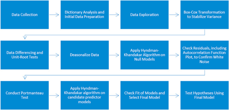
In this section the various steps in the research process are delineated. The study used dictionaries to analyze Twitter data from the US and official US data on the number of COVID-19 cases, combined with dynamic regression via ARIMA modelling in R. The steps in the research process are outlined in Fig. 1 . In the next section, we examine the benefits of using ARIMA analysis. Subsequently, the paper examines the steps in the research process in more detail.
Fig. 1.
Research process.
3.1. Dynamic regression using ARIMA analysis
In this section, we examine the nature and abilities of ARIMA modeling, its benefits over other social science methods, and the necessary transformation of times series data for ARIMA modelling.
ARIMA is a stochastic time series model that is typically used to forecast future time series points. The econometric technique is widely used in finance and economics (Shumway and Stoffer, 2000; Tsay, 2010), but is less used in the social sciences. Notwithstanding, ARIMA has been applied in a wide array of applications in the social sciences (Box-Steffensmeier et al., 2014; Shin, 2017).
ARIMA is able to capture very complex relationships in the data through its combination of techniques (Box et al., 2015). The Wold decomposition theorem states that any covariance stationary process can be decomposed into two mutually uncorrelated processes, a linear combination of lags in a white noise process, and a process of future values predicted by a linear function of past observations (Papoulis and Pillai, 2002). The autoregressive (AR) aspect refers to lagged observations of time series used to forecast future observations weighted according to how recent the past terms are. The integrated (I) aspect refers to the removal of seasonality from time series to make it stationary (discussed further below). Finally, the moving average (MA) element refers the use of error terms from previous time points in predicting current and future observations. This process removes random movements from a time series. Residual seasonal components in the time series may also be taken into consideration in order to improve the accuracy of the model (seasonal AR and seasonal MA components – see section 3.3). ARIMA analysis may also include exogenous variables in order to improve the accuracy of models, and the relationship between independent and dependent variables may also be examined through “dynamic regression” using ARIMA errors (Hyndman and Athanasopoulos, 2018 – see section 3.4).
ARIMA differs from other longitudinal analysis techniques in the social sciences such as latent growth modelling (LGM) and multi-level modelling (MLM) in a number of ways. First, it focuses on a single-unit dependent variable over time. It is suitable in situations where there is suitable aggregate data for a phenomenon, but where individual data may be sparse or incomplete (as is the case in this study). Second, while LGM and MLM tend to be applied on data sets with only a few time periods, ARIMA is most suitable for time series with more than 50 time points (Yanovitzky and VanLear, 2007). Third, neither LGM or MLM adequately reflect the time series character of a data set and do not capture trends that are caused by the internal dynamics of the variable under study (Hollanders and Vliegenthart, 2008). This limitation is typically addressed via research designs with a small number of distinct time data points (often two, three or four) or with panel data sets (Shin, 2017). Notwithstanding, a key problem in such designs is that variables are expected to vary at random, so the common practice of selecting data every three or four time units (Wilson et al., 2006), can easily result in the incorrect identification of a trend (Kelly and McGrath, 1988). ARIMA is designed to account for the complex internal dynamics of time series variables through the different mechanisms it employs, as explained above.
ARIMA focuses on determining underlying relationships for variables in the data set. Therefore, it is important that observations are not dependent on the time at which they are taken. If there are seasonal effects or trends that depend on the time index, any analysis of relationships between variables will be heavily biased and inaccurate. Thus, ARIMA requires wide-sense stationarity, whereby the mean and variance or autocovariance are constant over time, implying that variance is not a function of time (homoscedasticity) and there is no pattern in covariance over time. Typically, a time series has systematic short-term fluctuations rather than random variations around a trend; such systematic patterns in the time series variables must be removed in order to accurately test the relationship between them, since correlations may simply be a product of the patterns (Shin, 2017). Thus, where necessary, time series data is transformed to make it stationary. This fulfils the criteria of the Wold theorem and enables modelling in the absence of systematic time bias.
3.2. Data collection, dictionary analysis, data preparation and exploration
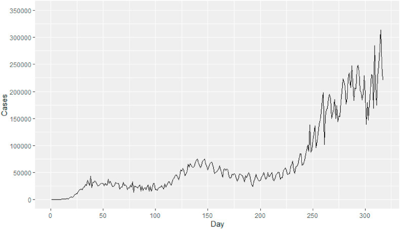
This paper concentrated on Twitter user data from the US during the pandemic. Tweets related to COVID-19 posted during the period from the January 20, 2020 to the January 10, 2021 were downloaded. Tweets were identified using the tweet IDs collected by Banda et al. (2021),.1 The entire corpus of tweet IDs was downloaded and then filtered for US tweets identified as being written in English (note: both are variables in the downloaded corpus). This study focused on the original tweets and did not consider retweets, to avoid double-counting. A total of 762,627 anonymized tweets were captured during this process (other tweets during this period were either not coded as “US” or “English” or no longer unavailable for download). Data on daily diagnosed COVID-19 cases was downloaded from the website of the Centers for Disease Control and Prevention (CDC, 2021). The early period that contained predominantly zero case data was excluded, up to and including the February 28, 2020, which was the last day in the data window reporting a zero daily case rate. The time series of US COVID-19 cases is illustrated in Fig. 2 . This appears to show weekly seasonality (i.e. a sawtooth pattern) and a number of interim peaks, including after Easter, Independence Day, Thanksgiving and Christmas.
Fig. 2.
COVID-19 cases in the US (February 29, 2020 to January 10, 2021).
For past, present and future temporal focus the relevant dictionaries from LIWC2015 (Pennebaker et al., 2015a, 2015b, 2015b) were used. LIWC2015 contains approximately 6400 words across numerous categories. It includes 862 words related to time orientation, including 341 for past focus (e.g., ago, did, and talked), 424 for present focus (e.g. today, is, and now), and 97 for future focus (e.g., may, will, and soon) (Pennebaker et al., 2005b).
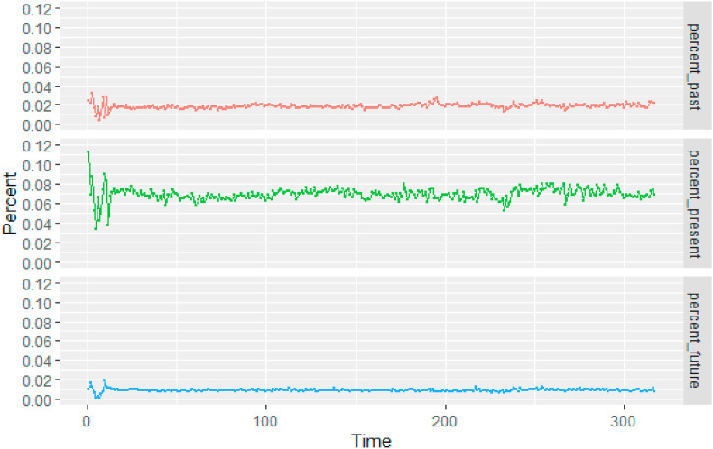
The analysis produced scores for each tweet, related to each word dictionary (“Past”, “Present” and “Future” temporal focus). Using the raw scores and word counts for each tweet, the number of words relating to each dictionary were then calculated for each tweet. Thus, each tweet may contain words with past, present and/or future focus. Overall, there were 217,767 tweets with at least one past-focused word, 508,062 with at least one present-focused word, and 136,946 with at least one future-focused word. Subsequently, construct count and COVID-19 case data were then aggregated into a daily time series format suitable for ARIMA analysis. This process involved calculating the percentage of total words with each type of temporal focus on each day in the time window. Descriptive statistics on the data set are given in Table 1 . This shows that a present temporal focus was the most common (mean of 6.93%), followed by a past focus (mean of 1.86%). A future focus was much less common (mean of 0.90%).
Table 1.
Descriptive statistics on data set.
| Variable | Days | Daily Minimum | Daily Maximum | Daily Mean | Std. Error | Std. Deviation |
|---|---|---|---|---|---|---|
| Past | 317 | 0.42% | 3.20% | 1.86% | .00015 | .00260 |
| Present | 317 | 3.31% | 11.27% | 6.93% | .00036 | .00645 |
| Future | 317 | 0.15% | 1.90% | 0.90% | .00008 | .00139 |
| COVID-19 Cases | 317 | 6 | 314,093 | 73579.79 | 3928.24 | 70708.30 |
The time series for the temporal focus variables used in the dynamic regression analysis are illustrated in Fig. 3 . It is difficult to discern relationships between the variables from this without statistical analysis.
Fig. 3.
COVID-19 cases and temporal focus.
3.3. Stabilizing variance, stationarity and seasonality
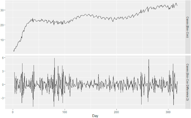
As we can see from Fig. 2, there appear to be considerable differences in variance for the number of COVID-19 cases in the US over the times series. In these situations, Hyndman and Athanasopolous (2018) recommend applying a Box-Cox transformation to stabilize the variance. The value of lambda for the Box-Cox transformation was calculated as 0.13972 using the forecast package in R. Accordingly, a Box-Cox transformation was applied to the COVID-19 case data and the resulting time series is shown in Fig. 4 , which has a considerably more stabilized variance.
Fig. 4.
Box-cox transformed and differenced case data.
The ndiffs procedure in the forecast package suggested that two orders of differences were required for stationarity. In order to assess whether the number of COVID-19 cases becomes stationary after two levels of differences, we applied the Kwiatkowski-Phillips-Schmidt-Shin (KPSS) test (Kwiatkowski et al., 1992). The KPSS Unit Root Test (mu with 5 lags) resulted in a test statistic of 0.017, well below the critical value of 0.463 for the 5% significance level. This suggests that the data set is stationary and that no further differencing in the data is required. The differenced data is shown in Fig. 4, which now appears much like white noise.
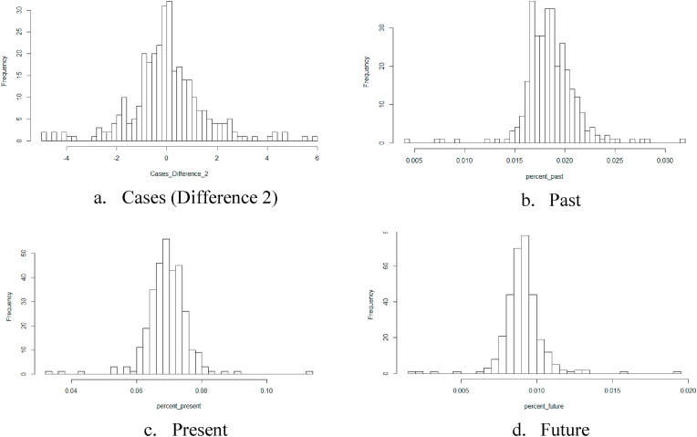
Fig. 5 displays histograms of the frequency distributions of the variables used in the analysis. Normality of the variables is not a requirement of ARIMA analysis. .
Fig. 5.
Distribution of variables used in the analysis.
In order to confirm that the time series is stationary, the autoarima procedure (Hyndman and Khandakar, 2008) was applied to the differenced case data and the residuals were examined. The result of the analysis is shown as “Model 0: Null Model” in Table 2 . The procedure selected an ARIMA(3,0,2) model with zero mean as the best fit using the maximum likelihood procedure (suggesting no differencing in the dependent variable, since this has already been dealt with – as discussed above). A non-seasonal ARIMA(p,d,q) model is given by the equation:
| (1) |
Where refers to a white noise process, Ν(0, σ2), B is the backshift operator, (B) = () (the autoregressive or AR components), and = () (the moving average or MA components). Thus, for the resulting model with zero mean this becomes:
| (2) |
Where =(1-B)d Yt. Three autoregressive coefficients are identified in the model, with two of them being significant, AR1 ( p<.01) and AR3 ( p<.001). In addition, the two moving average coefficients, MA1 () and MA2 () are both significant at the 0.1% level. Given that the data has already been differenced twice before analysis, so yt=(1-B)2 Yt, the equation of the resulting model is:
| (3) |
Table 2.
Null models.
| Term | Model 0: Null Model |
Model 0d: De-seasonalized Null Model |
|---|---|---|
| AR1 | 0.23** (0.07) | |
| AR2 | 0.00 (0.06) | |
| AR3 | −0.22*** (0.06) | |
| MA1 | −1.67*** (0.06) | −1.56*** (0.04) |
| MA2 | 0.75*** (0.05) | 0.61*** (0.05) |
| SMA1 | 0.17** (0.06) | |
| σ2 | 0.68 | 0.53 |
| AIC | 782.36 | 704.93 |
| AICc | 782.63 | 705.06 |
| BIC | 804.88 | 719.94 |
| Log Likelihood | −385.18 | −348.47 |
| n | 315 | 315 |
***p < 0.001; **p < 0.01; *p < 0.05.
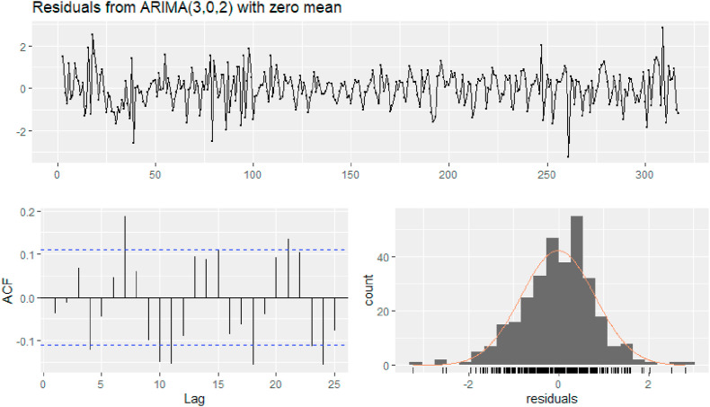
Residual diagnostics are provided in Fig. 6 . Here we can see that the autocorrelation function (ACF or correlogram) identifies numerous lags that are outside of the 95% range identified by the blue dashed lines, suggesting that this is not a white noise series. In order to confirm that this is not a false positive result, a portmanteau test was conducted – the Ljung-Box test (Ljung and Box, 1978), which is considered more accurate than the related Box-Pierce test (Box and Pierce, 1970; Box et al., 2015). The Ljung-Box Q* was 31.233, which is significant at the 0.1% level (df = 5, total lags used = 10), suggesting that the data is not white noise and is therefore not yet stationary. The residuals plot suggested potential weekly seasonality in case numbers; therefore, a seasonal decomposition was conducted.
Fig. 6.
Residual diagnostics for null model.
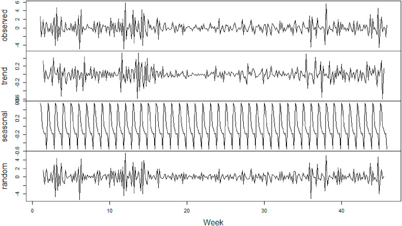
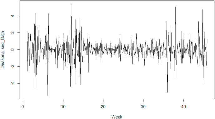
Fig. 7 shows the result of decomposing the case variable based on an additive time series. As we can see from the third window, there is a clear weekly seasonal component in the data. Therefore, this component was removed (subtracted) from the differenced time series (see Fig. 8 ) and the autoarima procedure was conducted on the revised data set. The resulting model is shown as “Model 0d: De-seasonalized Null Model” in Table 2. This is an ARIMA(0,0,2)(0,0,1)[7] model. The general form of a seasonal ARIMA(p,d,q)(P,D,Q)[m] model is:
| (4) |
where m is the time span of the seasonal pattern, (Bm) = () (seasonal AR components), and = () (seasonal MA components). Thus, Model 0d is equivalent to the model:
| (5) |
Fig. 7.
Decomposition of additive time series.
Fig. 8.
De-seasonalized case data.
This new model retained the moving average terms MA1 () and MA2 () at similar levels and at the 0.1% level of significance. However, a new weekly seasonal moving average term was introduced into the model, SMA1 (), which is significant at the 1% level. Given that , the equation of the new model can be simplified as:
| (6) |
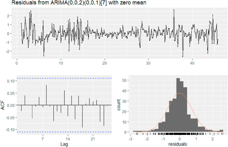
Fig. 9 provides the residual diagnostics for Model 0d. The autocorrelation function showed clearly that the data for the lags was well within the 95% range. This was further confirmed by a Ljung-Box test: Q* = 8.038, df = 11, p = 0.710 (model df = 3; total lags used = 14).
Fig. 9.
Residual diagnostics for de-seasonalized null model.
Table 2 also examines the fit of the null and de-seasonalized null models. As we can see, the de-seasonalized model clearly has a better fit with the data, with a higher Log-Likelihood (logLik = −348.5; 36.7 higher than the null model) and a lower value for the corrected Akaike Information Criterion (AICc = 705.1; 77.6 lower than the null model) and Bayesian Information Criterion (BIC = 719.9; 85.0 lower than the null model). Thus, we will proceed with using the de-seasonalized null model for further analysis.
3.4. Testing and Evaluating the dynamic regression Models and hypotheses
Once the time series had been prepared for dynamic regression, a number of candidate models were examined via the autoarima procedure. Dynamic regression involves estimating a regression using ARIMA errors, but requires that the variables are stationary, as we have confirmed in section 3.2. The general form of a dynamic regression model measured with ARIMA errors is given by:
| (7) |
and
| (8) |
where k is the number of predictors in the model and is the error series that is assumed to follow an ARIMA model. Thus, we have two error terms: the error from a regression model, , and the error from the ARIMA model, . Whilst ARIMA model errors are assumed to be white noise, regression model errors are not, and are used for purposes of prediction.
The autoarima procedure selects the model that fits best according to the ARIMA errors and differences any variables that need it (such as the independent variables in our models). The AICc is computed for the final model, which can then be used to determine which predictors in candidate models should be used. The procedure should be run for all subsets of predictors to be considered, and the model with the lowest AICc value is then selected (Hyndman and Athanasopolous, 2018).
Statistical modelling applied seven candidate ARIMA models to the data: three single predictor models (Model 1: Past, Model 2: Present, and Model 3: Future), three dual predictor models (Model 4: Past & Present, Model 5: Present & Future, and Model 6: Past & Future), and the full model with all three predictors (Model 7). The specific models tested using dynamic regression were:
-
•
Model 1:
| (9) |
-
•
Model 2:
| (10) |
-
•
Model 3:
| (11) |
-
•
Model 4:
| (12) |
-
•
Model 5:
| (13) |
-
•
Model 6:
| (14) |
-
•
Model 7:
| (15) |
Fit metrics (AICc, BIC and Log-Likelihood) were examined to identify the model that fits best with the data. The final model was then examined using residual diagnostics and the portmanteau test. The selected model was then examined further using a z-test of the coefficients in the full dynamic regression model. The p-value of the z-test coefficients was then used as the basis for hypothesis testing.
4. Results of dynamic regression modelling
The seven candidate models were tested using the autoarima algorithm in the forecast package and in each case an ARIMA(0,0,2)(0,0,1)[7] model was selected by the procedure. The results of model testing are shown in Table 3 .
Table 3.
Dynamic linear regression models for predictor combinations.
| Model 1: Past |
Model 2: Present |
Model 3: Future |
Model 4: Past & Present | Model 5: Present & Future | Model 6: Past & Future | Model 7: All Three Predictors |
|
|---|---|---|---|---|---|---|---|
| MA1 | −1.56*** | −1.56*** | −1.56*** | −1.57*** | −1.57*** | −1.55*** | −1.59*** |
| (0.04) | (0.04) | (0.04) | (0.04) | (0.05) | (0.04) | (0.04) | |
| MA2 | 0.60*** | 0.61*** | 0.61*** | 0.61*** | 0.62*** | 0.59*** | 0.63*** |
| (0.05) | (0.05) | (0.05) | (0.04) | (0.05) | (0.05) | (0.05) | |
| SMA1 | 0.18** | 0.17** | 0.17** | 0.19** | 0.17** | 0.18** | 0.19** |
| (0.06) | (0.06) | (0.06) | (0.06) | (0.06) | (0.06) | (0.06) | |
| Intercept | −0.07* | ||||||
| (0.03) | |||||||
| Past | 3.57* | 4.95** | 3.01* | 5.64*** | |||
| (1.71) | (1.51) | (1.32) | (1.62) | ||||
| Present | −0.02 | −1.35*** | −0.64 | −2.68* | |||
| (0.04) | (0.40) | (0.96) | (1.07) | ||||
| Future | −0.18 | 4.73 | −6.34* | 8.78 | |||
| (0.29) | (7.32) | (2.70) | (6.50) | ||||
| σ2 | 0.53 | 0.54 | 0.54 | 0.52 | 0.54 | 0.53 | 0.52 |
| AIC | 704.93 | 706.51 | 706.55 | 700.40 | 708.10 | 704.71 | 700.58 |
| AICc | 705.20 | 706.71 | 706.74 | 700.68 | 708.37 | 704.99 | 700.95 |
| BIC | 727.45 | 725.28 | 725.31 | 722.92 | 730.62 | 727.23 | 726.85 |
| Log-Lik. | −346.47 | −348.26 | −348.27 | −344.20 | −348.05 | −346.36 | −343.29 |
| Num. obs. | 315 | 315 | 315 | 315 | 315 | 315 | 315 |
| Q* | 8.72 (n.s.) | 8.05 (n.s.) | 8.06 (n.s.) | 9.11 (n.s.) | 7.81 (n.s.) | 9.40 (n.s.) | 8.42 (n.s.) |
***p < 0.001; **p < 0.01; *p < 0.05; n.s. not significant; standard error in brackets; autoarima algorithm automatically identified ARIMA(0,0,2)(0,0,1)[7] for each candidate model.
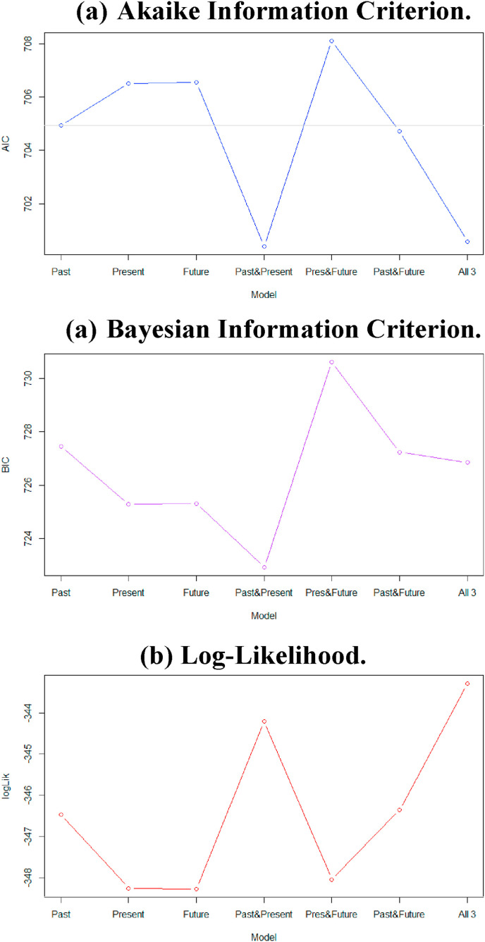
Fig. 10 shows a comparison of model fit for the three single predictor variable models (Models 1 to 3), three dual-predictor models (Models 4 to 6) and the full three-variable ARIMA model (Model 7). As we can see, the fit for the dual model with the past and present predictor variables appears superior for two of the metrics (AIC/AICc and BIC, although the margin is very small for AIC/AICc), while the full model with three variables is marginally better for the Log-Likelihood metric. The Past, Present, Future and Present & Future models had values of AICc higher than that of the null de-seasonalized model, indicating a poor fit. The Past & Present model (Model 4), however, had an AICc value of 700.68 and a BIC value of 722.92, indicating a stronger fit with the data. The full model (Model 7) had an AICc value of 700.95 and a BIC of 726.85, indicating a slightly weaker fit. Although the Log-Likelihood for Model 7 is closer to zero than Model 4 (−343.29 versus −344.20 respectively), Hyndman and Athanasopoulos (2018) consider this less important than the AICc metric and recommend using AICc in order to determine the best model predictors from those available. Thus, the best model is considered to be Model 4, with past and present temporal focus predictors.
Fig. 10.
Comparison of model fit for variable combinations in models.
The statistical analyses for hypothesis testing using the dynamic linear regression are also shown in Table 3. This provides the significance level of the models’ terms from a z-test of the coefficients used in the ARIMA models. As we can see, Model 4 has two significant moving averages at the p<.001 level, MA1 and MA2, and a small seasonal moving average that is significant can the p<.01 level, SMA1. This indicates that there is a small but significant amount of residual seasonality that is picked-up by the automatic ARIMA procedure.
Regarding the temporal focus predictor variables, the coefficient test show that past focus has a direct and significant effect on the number of COVID-19 cases at the 1 percent level (β1 = 4.95, p = 0.001). This provides support for Hypothesis 1. Further, the z-test of the coefficient for present temporal focus shows that it has a more significant but smaller (in absolute terms) inverse impact on the number of COVID-19 cases at the 0.1 percent level (β2 = −1.35, p < 0.001). Thus, support is also provided for Hypothesis 2. However, the predictor for future temporal focus does not appear in this model and therefore no support is offered for Hypothesis 3. This is likely to be due to insufficient data for temporal focus in the data set, and furthermore, Model 7 shows an extremely high standard error for future focus.
In other words, the difference in the differences in the number of COVID-19 cases can be partly explained by the temporal focus of citizens, measured through a big data set of tweets as a proxy of the nation's overall perspective. In terms of the predictive quality of the final model, the squared correlation between the fitted values of Model 4 and the dependent variable used in the analysis (similar to R-squared) is 0.76, suggesting a good predictive value of the model; 76% of the value of the data is captured by the fitted model.
5. Discussion and conclusions
This research suggests that temporal focus, measured through big data analytics and longitudinal analysis of social media text data, influences the spread of COVID-19. Using a large data set of more than three-quarters of a million tweets tagged with COVID-19-related terms during the pandemic, the level of temporal focus was calculated using text analytics over a 317-day period. Using econometric methods, the data was prepared and then tested using ARIMA modelling and the best fitting models selected and examined via dynamic regression. Various statistical checks found the final model to be robust. The findings show that past temporal focus has a significant direct effect on the change in diagnosed COVID-19 cases over time, providing support for hypothesis 1. On the other hand, the results also demonstrate that a present temporal focus has a significant inverse effect on the change in diagnosed COVID-19 cases over time, providing support for hypothesis 2. No support was found for hypothesis 3, relating to the impact of a future temporal focus, and this is likely to be due to a lack of data measuring this aspect in the time window. The limited data could potentially be due to the dictionary approach used, since the LIWC2015 dictionary contains fewer future-focused words than those of past or present focus. Let us examine the implications of these findings for research and practice.
One of the key contributions of this research is the development of a research process for the application of big data and advanced data analytics (outlined in Fig. 1) in order to improve understanding of the effects of temporal focus on human behavior. Shipp and Aeon (2019) note that big data and advanced analytics provides a new and unobtrusive way to study temporal focus by coding text and call for more research applying such techniques. This study answers this call and provides an original, unified research process that can be used to formally examine the impacts of temporal focus on outcome variables using combined text analytics and time series dynamic regression.
A second key contribution of this paper is in our theoretical understanding of the Temporal Focus Hypothesis. This paper offers early, large-scale, text-based empirical evidence of a relationship between past temporal focus and infection rates. This finding would seem consistent with a past negative time perspective (Zhang and Howell, 2011; Zimbardo and Boyd, 1999). Not all members of society adhere to regulations and guidance regarding health behavior and COVID-19 (Li et al., 2020; Wang et al., 2020; Zajenkowski et al., 2020), particularly in the early stages of the pandemic when signs of illness are not immediately obvious in their immediate environment (Makhanova and Shepherd, 2020). This research supports the general assertion by Shipp et al. (2019) regarding the impacts of past focus that have been found in numerous other studies. In the context of the pandemic, past temporal focus has a direct relationship with infection rates. On the other hand, a strong present focus has an inverse relationship with infection rates. This directly supports the findings of Sobol-Kwapinska et al. (2020) relating to a positive correlation between a present temporal focus and compliance with public health regulations concerning COVID-19. More generally, it supports studies that find that a present focus tends to have a positive impact (e.g., Rush and Grouzet, 2012; Tseferifi et al., 2017). This would appear consistent with a Carpe Diem time perspective (Sobol-Kwapinska et al., 2020; Tseferidi et al., 2017). Unfortunately, the study did not find that a future temporal focus had a significant relationship with infection rates. This is a surprising finding that is likely to be due to a lack of data. Future focus deserves greater scrutiny in future studies investigating COVID-19 and infection rates using big data analytics.
This study contributes useful findings that are relevant to the practice of public health policy. Improving citizens' response to public health measures requires a better understanding of the determinants of behaviors to understand which individuals are likely to flout the rules and which are likely to follow them. The understanding of temporal focus as a driver of infection enables more effective development of two aspects of public health policy. First, by identifying these significant determinants of changes in COVID-19 cases, it provides additional metrics to improve the development of epidemiological models to better understand the spread of the disease (and other diseases). Second, by understanding the inverse relationship of present focus and the direct relationship of past focus on case rates it contributes to the framing of more effective public health messages targeted at citizens in order to attempt to improve compliance with regulations and guidance. Given that temporal focus is malleable in many individuals (in Rush and Grouzet's (2012) study temporal focus varied by around two-thirds on a daily basis), messages should be designed in order to elicit a present temporal focus to help induce behaviors assisting compliance and a reduction in case rates.
This study has a number of limitations. The data set contained inadequate data on future temporal focus and more data is needed to measure the impact of this variable. It is possible that the content of tweets may be distinct from an individual's actual temporal orientation (e.g., the nature of tweeting may be a more immediate/present oriented activity, where people are tweeting about current happenings). At the time of this research, although vaccines have been developed and are being administered in the US and elsewhere, for the time being, the pandemic continues. Thus, the data window of ten months does not capture fully the entirety of the pandemic, and future research should consider extending the time window. Moreover, the study includes only Twitter messages (tweets) identified as being written in English and in the United States. Temporal focus could be further examined on other social media platforms, in other countries, and in other languages. Tweets without an identified language but with an identified country could be further processed to identify the language used.
It is possible that other confounding factors may have influenced the results that have not been captured in the research. For example, there are many policy changes that took place during the study period that may have affected both temporal focus and infections rates. Another limitation of the research is that it does not examine emotional attitudes to specific time areas or differentiate between the past negative and past positive perspective or between the future positive and future negative perspective. These aspects present opportunities for future research. Furthermore, other factors such as age have been found to be related to temporal focus (Bylund et al., 2020) and age is also likely to be related to the incidence of COVID-19 cases. Individuals using Twitter most frequently may not be representative of the general population. For example, Twitter usage varies by age group, although it has developed significantly in recent years; according to Tankovska (2021), Twitter usage penetration is now 26% for those aged 56 years or more, compared to 39% for 46–55 years, 43% for 36–45 years, and 48% for 26–35 years of age. Future studies should seek to investigate the impact of age in moderating the impact of temporal focus on the changing rate of diagnosed COVID-19 cases.
Credit author statement
Sole authored work: All aspects completed by the author.
Footnotes
Banda et al. (2021) have developed a resource that regularly collects tweet IDs for posts containing common COVID-19-related terms, including wuhanvirus, covid-19, COVD19, 2019nCoV, CoronavirusPandemic, COVID-19, WuhanVirus, CoronaOutbreak, covid19, coronavirus, coronaoutbreak, and coronaviruspandemic2019ncov.
References
- Banda J.M., Tekumalla R., Wang G., Yu J., Liu T., Ding Y., Artemova K., Tutubalina R., Chowell G. A large-scale COVID-19 Twitter chatter dataset for open scientific research. An international collaboration. 2021 doi: 10.5281/zenodo.3723939. 14th January, 2021. [DOI] [PMC free article] [PubMed] [Google Scholar]
- Barnes S.J., Mattsson J., Sørensen F., Jensen J.F. Measuring and enhancing the experiential value of employee-tourist encounters: a big data analytics approach. Expert Syst. Appl. 2020;154:113450. [Google Scholar]
- Baumsteiger R. Looking forward to helping: the effects of prospection on prosocial intentions and behavior. J. Appl. Soc. Psychol. 2017;47:505–514. [Google Scholar]
- Bluedorn A.C. Stanford Business Books; Stanford, CA: 2002. The Human Organization of Time: Temporal Realities and Experience. [Google Scholar]
- Box G.E.P., Pierce D.A. Distribution of residual autocorrelations in autoregressive-integrated moving average time series models. J. Am. Stat. Assoc. 1970;65(332):1509–1526. [Google Scholar]
- Box G.E.P., Jenkins G.M., Reinsel G.C., Ljung G.M. fifth ed. John Wiley & Sons; Hoboken, New Jersey: 2015. Time Series Analysis: Forecasting and Control. [Google Scholar]
- Box-Steffensmeier J.M., Freeman J.R., Hitt M.P., Pevehouse J.C.W. Cambridge University Press; New York: 2014. Time Series Analysis for the Social Sciences. [Google Scholar]
- Brosnan K., Babkhani N., Dolcinar S. “I know what you’re going to ask me” Why respondents don't read survey questions. Int. J. Mark. Res. 2019;61(4):366–379. [Google Scholar]
- Bruderer Enzler H. Consideration of future consequences as a predictor of environmentally responsible behavior: evidence from a general population study. Environ. Behav. 2015;47(6):618–643. [Google Scholar]
- Bylund E., Gygax P., Samuel S., Athanasopoulos P. Back to the future? The role of temporal focus for mapping time onto space. Q. J. Exp. Psychol. 2020;73(2):174–182. doi: 10.1177/1747021819867624. [DOI] [PubMed] [Google Scholar]
- Cartwright D., editor. Field Theory in Social Science: Selected Theoretical Papers by Kurt Lewin. Harper & Row; New York: 1951. [Google Scholar]
- CDC COVID data tracker. 2021. https://covid.cdc.gov/covid-data-tracker/ accessed 5th February, 2021.
- CRC . Johns Hopkins University; 2021. COVID-19 Dashboard. Coronavirus Resource Center.https://coronavirus.jhu.edu/map.html accessed 5th February 2021. [Google Scholar]
- Daugherty J.R., Brase G.L. Taking time to be healthy: predicting health behaviors with delay discounting and time perspective. Pers. Indiv. Differ. 2010;48(2):202–207. [Google Scholar]
- de la Fuente J., Santiago J., Roman A., Dumitrache C., Casasanto D. When you think about it, your past is in front of you: how culture shapes spatial conceptions of time. Psychol. Sci. 2014;25:1682–1690. doi: 10.1177/0956797614534695. [DOI] [PubMed] [Google Scholar]
- De Vaus D.A. fourth ed. UCL Press; London: 1996. Surveys in Social Research. [Google Scholar]
- Dillman D.A., Smyth J.D., Christian L.M. fourth ed. John Wiley & Sons; Hoboken: 2014. Internet, Phone, Mail, and Mixed-Mode Surveys: the Tailored Design Method. [Google Scholar]
- Griva F., Tseferidi S.-I., Anagnostopoulos F. Time to get healthy: associations of time perspective with perceived health status and health behaviors. Psychol. Health Med. 2015;20(1):25–33. doi: 10.1080/13548506.2014.913798. [DOI] [PubMed] [Google Scholar]
- Hofstede G., Hofstede G.J., Minkov M. third ed. McGraw-Hill; New York: 2010. Cultures and Organizations: Software of the Mind. [Google Scholar]
- Hollanders D., Vliegenthart R. Telling what yesterday's news might be tomorrow: modeling media dynamics. Communications. 2008;33:47–68. [Google Scholar]
- Hyndman R.J., Athanasopoulos G. second ed. 2018. Forecasting: Principles and Practice. OTexts: Melbourne. OTexts.com/fpp2. 4th September, 2020. [Google Scholar]
- Hyndman R.J., Khandakar Y. Automatic time series forecasting: the forecast package for R. J. Stat. Software. 2008;27(1):1–22. [Google Scholar]
- Ireland M.E., Schwartz H.A., Chen Q., Ungar L.H., Albarracín D. Future-oriented tweets predict lower county-level HIV prevalence in the United States. Health Psychol. 2015;34(Suppl. l):1252–1260. doi: 10.1037/hea0000279. [DOI] [PMC free article] [PubMed] [Google Scholar]
- Jovancevic A., Milicevic N. Optimism-pessimism, conspiracy theories and general trust as factors contributing to COVID-19 related behavior: a cross-cultural study. Pers. Indiv. Differ. 2020;167:110216. doi: 10.1016/j.paid.2020.110216. [DOI] [PMC free article] [PubMed] [Google Scholar]
- Kelly J.R., McGrath J.E. Sage Publications; Newbury Park, CA: 1988. On Time and Method. [Google Scholar]
- Keough K.A., Zimbardo P.G., Boyd J.N. Who's smoking, drinking, and using drugs? Time perspective as a predictor of substance use. Basic Appl. Soc. Psychol. 1999;21:149–164. [Google Scholar]
- Kwiatkowski D., Phillips P.C.B., Schmidt P., Shin Y. Testing the null hypothesis of stationarity against the alternative of a unit root: how sure are we that economic time series have a unit root? J. Econom. 1992;54(1–3):159–178. [Google Scholar]
- Laureiro-Martinez D., Trujillo C.A., Unda J. Time perspective and age: a review of age associated differences. Front. Psychol. 2017;8:101. doi: 10.3389/fpsyg.2017.00101. accessed 10th February, 2021. [DOI] [PMC free article] [PubMed] [Google Scholar]
- Li H. A future-minded lark in the morning: the influence of time-of-day and chronotype on metaphorical associations between space and time. Metaphor Symbol. 2018;33:48–57. [Google Scholar]
- Li S., Wang Y., Xue J., Zhao N., Zhu T. The impact of COVID-19 epidemic declaration on psychological consequences: a study on active Weibo users. Int. J. Environ. Res. Publ. Health. 2020;17(6):2032. doi: 10.3390/ijerph17062032. [DOI] [PMC free article] [PubMed] [Google Scholar]
- Li H., Cao Y. In times of illness: covid-19 threat influences temporal focus and implicit space-time mappings. Pers. Indiv. Differ. 2021;171:110561. doi: 10.1016/j.paid.2020.110561. [DOI] [PMC free article] [PubMed] [Google Scholar]
- Ljung G.M., Box G.E.P. On a measure of a lack of fit in time series models. Biometrika. 1978;65(2):297–303. [Google Scholar]
- Makhanova A., Shepherd M. Behavioral immune system linked to responses to the threat of COVID-19. Pers. Indiv. Differ. 2020;167:1–7. doi: 10.1016/j.paid.2020.110221. [DOI] [PMC free article] [PubMed] [Google Scholar]
- Milfont T.L., Wilson J., Diniz P. Time perspective and environmental engagement: a meta‐analysis. Int. J. Psychol. 2012;47:325–334. doi: 10.1080/00207594.2011.647029. [DOI] [PubMed] [Google Scholar]
- Papoulis A., Pillai U. McGraw-Hill; New York: 2002. Probability, Random Variables, and Stochastic Processes. [Google Scholar]
- Park G., Schwartz H.A., Sap M., Kern M.L., Weingarten E., Eichstaedt J.C., Berger J., Stillwell D.J., Kosinski M., Ungar L.H., Seligman M.E.P. Living in the past, present, and future: measuring temporal orientation with language. J. Pers. 2017;85:270–280. doi: 10.1111/jopy.12239. [DOI] [PubMed] [Google Scholar]
- Pennebaker J.W., Booth R.J., Boyd R.L., Francis M.E. Pennebaker Conglomerates; Austin, TX: 2015. Linguistic Inquiry and Word Count: LIWC2015.www.LIWC.net [Google Scholar]
- Pennebaker J.W., Boyd R.L., Jordan K., Blackburn K. University of Texas at Austin; Austin, TX: 2015. The Development and Psychometric Properties of LIWC2015. [Google Scholar]
- Przepiorka A., Blachnio A. Time perspective in Internet and Facebook addiction. Comput. Hum. Behav. 2016;60:13–18. [Google Scholar]
- Podsakoff P.M., MacKenzie S.B., Lee J.-Y., Podsakoff N.P. Common method biases in behavioral research: a critical review of the literature and recommended remedies. J. Appl. Psychol. 2003;88(5):879–903. doi: 10.1037/0021-9010.88.5.879. [DOI] [PubMed] [Google Scholar]
- Rappaport H. Simon & Schuster; New York: 1990. Marking Time. [Google Scholar]
- Rothspan S., Read S.J. Present versus future time perspective and HIV risk among heterosexual college students. Health Psychol. 1996;15:131–134. doi: 10.1037//0278-6133.15.2.131. [DOI] [PubMed] [Google Scholar]
- Rush J., Grouzet F.M.E. It is about time: daily relationships between temporal perspective and well-being. J. Posit. Psychol. 2012;7(5):427–442. [Google Scholar]
- Sergent J., Padilla R. The U.S. COVID-19 death toll now exceeds 406,000. That's more than the number of Americans who died in WWII. USA Today, January. 2021;19:2021. https://eu.usatoday.com/in-depth/news/2021/01/19/covid-19-deaths-americans-dying-faster-than-our-soldiers-did-wwii/6602717002/ 5th February 2021. [Google Scholar]
- Shin Y. University of California Press; Oakland, CA: 2017. Time Series Analysis in the Social Sciences: the Fundamentals. [Google Scholar]
- Shipp A.J., Edwards J.R., Schurer Lambert L. Conceptualization and measurement of temporal focus: the subjective experience of the past, present, and future. Organ. Behav. Hum. Decis. Process. 2009;110(1):1–22. [Google Scholar]
- Shipp A.J., Aeon B. Temporal focus: thinking about the past, present, and future. Current Opinion in Psychology. 2019;26:37–43. doi: 10.1016/j.copsyc.2018.04.005. [DOI] [PubMed] [Google Scholar]
- Shumway R.H., Stoffer D.S. Springer Texts in Statistics. Springer; New York, NY: 2000. Time Series Analysis and its Applications. [Google Scholar]
- Singleton R.A., Straits B.C. fifth ed. Oxford University Press; New York: 2009. Approaches to Social Research. [Google Scholar]
- Sobol-Kwapinska M., Jankowski T. Positive time. Balanced time perspective and positive orientation. J. Happiness Stud. 2016;17(4):1511–1528. [Google Scholar]
- Sobol-Kwapinska M., Blachnio A., Przepiórka Time of pandemic: temporal perspectives related to compliance with public health regulations concerning the COVID-19 pandemic. Soc. Sci. Med. 2020;265:113408. doi: 10.1016/j.socscimed.2020.113408. [DOI] [PMC free article] [PubMed] [Google Scholar]
- Stolarski M., Matthews G., Postek S., Zimbardo B.G., Bitner J. How we feel is a matter of time: relationships between time perspectives and mood. J. Happiness Stud. 2014;15:809–827. [Google Scholar]
- Stolarski M., Matthews G. Time perspectives predict mood states and satisfaction with life over and above personality. Curr. Psychol. 2016;35:516–526. doi: 10.1007/s12144-016-9515-2. [DOI] [PMC free article] [PubMed] [Google Scholar]
- Tankovska H. Twitter usage penetration in the United States 2020, by age group. 2021. https://www.statista.com/statistics/227175/daily-us-twitter-users-by-age-group/ March 24th, 2021.
- Trope Y., Liberman N. Temporal construal. Psychol. Rev. 2003;110:403–421. doi: 10.1037/0033-295x.110.3.403. [DOI] [PubMed] [Google Scholar]
- Tsay R.S. John Wiley & Sons; Hoboken, NJ: 2010. Analysis of Financial Time Series. [Google Scholar]
- Tseferidi S.I., Griva F., Anagnostopoulos F. Time to get happy: associations of time perspective with indicators of well-being. Psychol. Health Med. 2017;22(5):618–624. doi: 10.1080/13548506.2016.1226508. [DOI] [PubMed] [Google Scholar]
- Wang C., Pan R., Wan X., Tan Y., Xu L., Ho C.S., Ho R.C. Immediate psychological responses and associated factors during the initial stage of the 2019 coronavirus disease (COVID-19) epidemic among the general population in China. Int. J. Environ. Res. Publ. Health. 2020;17(5):1729. doi: 10.3390/ijerph17051729. [DOI] [PMC free article] [PubMed] [Google Scholar]
- Wilson I., Huttly S.R.A., Fenn B. A case study of sample design for longitudinal research: young lives. Int. J. Soc. Res. Methodol. 2006;9:351–365. [Google Scholar]
- Yanovitzky I., VanLear A. In: The SAGE Sourcebook of Advanced Data Analysis Methods for Communication Research. Hayes A.F., Slater M., Snyder L.B., editors. Sage Publications; Thousand Oaks, CA: 2007. Time series analysis. Traditional and contemporary approaches; pp. 89–124. [Google Scholar]
- Zajenkowski M., Jonason P., Leniarska M., Kozakiewicz Z. Who complies with the restrictions to reduce the spread of COVID-19? Personality and perceptions of the COVID- 19 situation. Pers. Indiv. Differ. 2020;166:1–6. doi: 10.1016/j.paid.2020.110199. [DOI] [PMC free article] [PubMed] [Google Scholar]
- Zaleski Z., Sobol-Kwapinska M., Przepiorka, Meisner M. Development and validation of the dark future scale. Time Soc. 2017;28(1):107–123. [Google Scholar]
- Zhang J.W., Howell R.T. Do time perspectives predict unique variance in life satisfaction beyond personality traits? Pers. Indiv. Differ. 2011;50:1261–1266. [Google Scholar]
- Zimbardo P.G., Boyd J.N. Putting time in perspective: a valid, reliable individual-differences metric. J. Pers. Soc. Psychol. 1999;77(6):1271–1288. [Google Scholar]


