Average saturation efficiency filter (ASEF) for CEST MRI study of stroke in Rodents

Abstract

Purpose:

The Average Saturation Efficiency Filter (ASEF) is a novel method of improving the specificity of CEST, however, there is a mismatch between the MT effect under high duty cycle and low duty cycle pulse trains. We explore measures of mitigation and the sensitivity and potential of ASEF imaging in phantoms and stroke rats.

Methods:

Simulation and nicotinamide phantoms in denatured protein were used to investigate the effect of different average saturation powers and MT pool parameters on matching coefficients used for correction as well as the ASEFR ratio (ASEFR) signal and baseline. Then, in vivo studies were performed in stroke rodents to further investigate the sensitivity and fidelity of ASEFR spectra.

Results:

Simulation and studies of nicotinamide phantoms show that the matching coefficient needed to correct the baseline MT mismatch is strongly dependent on the average saturation power. In vivo studies in stroke rodents show that the matching coefficient required to correct the baseline MT mismatch is different for normal versus ischemic tissue. Thus, a baseline-correction was performed to further suppress the residue MT mismatch. After correction of the mismatch, ASEFR achieved comparable contrast at 3.6 ppm between normal and ischemic tissue when compared to the APT* approach. Moreover, contrasts for 2.0 ppm and 2.6 ppm were also ascertainable from the same spectra.

Conclusion:

ASEF can improve the CEST signal specificity of slow exchange labile protons such as amide and guanidyl, with small loss to sensitivity. It has strong potential in the CEST imaging of various diseases.

Introduction

Chemical Exchange Saturation Transfer (CEST) imaging has been growing in traction as a tool to image molecular moieties¹, both exogenous and endogenous, that have exchangeable protons such as mobile proteins or peptides, glucose, glycogen, creatine and phosphocreatine (PCr). Compared to other spectroscopic magnetic resonance methods that are often limited by the small proton pool of molecular targets, the exchange of labile protons to bulk water in CEST imaging magnifies imaged signals allowing for better spatial and temporal resolution to spectroscopic alternatives. Moreover, CEST can provide information on more than just the targeted molecules but also environmental factors surrounding them such as pH^2–9 and temperature, creating opportunities for the use of CEST imaging in providing diagnostic and predictive value in the study of diseases such as tumors^2,10–18, stroke^{4,6,8,9,19–22}, neurodegenerative disease^23–25, as well as muscle and kidney diseases^5,15,26–34.

CEST imaging is commonly achieved by applying RF saturation in either a long continuous wave (CW) or a train of short pulses at the resonant frequency of a target molecular moiety followed by imaging readout of the bulk water signal attenuated by exchange. While this indirect method of measurement enhances sensitivity, the trade-off is sacrificing specificity. Cross-contamination between exchange sources makes CEST signals complex thereby complicating their interpretation. Early on, an asymmetry analysis was used to separate CEST signals from direct water saturation and the semi-solid MT effect³⁵. Though simple and fast, MT from semi-solid molecules is asymmetric so asymmetry analysis is ineffective in removing its contribution^19,36. Moreover, aliphatic protons on the negative side of the Z-spectrum attenuate signal through the transfer of saturation through the NOE effect further confounding the asymmetry analysis. To alleviate this problem, methods such as multi-Lorentzian fitting³⁷, Polynomial and Lorentzian Line-shape Fitting (PLOF)³⁰, 3-point measurement¹⁹, Chemical Exchange Rotation Transfer (CERT)^13,38,39, and Variable Delay Multi-Pulse (VDMP) imaging⁴⁰ have been developed to isolate CEST signals from their non-CEST background.

We have recently developed a novel method dubbed Average Saturation Efficiency Filter (ASEF) CEST imaging⁴¹. This approach utilizes a high duty cycle (DC) (or CW which has a maximal DC of 1) and a low DC binomial pulse train with similar average B₁ power deposition such that fast exchanges and the MT process have similar saturation transfer effects between both pulse schemes. In contrast, slow exchanges will have largely different saturation transfer effects between the two pulse schemes. Thus, the saturation transfer effects from fast exchanges and MT can be subtracted out between two signals saturated by each pulse train, leaving only the difference of their CEST signals which is mostly from slower exchange contributions.

Although the effectiveness of the exchange rate filtering effect has been confirmed in a pilot phantom study of ASEF signal⁴¹, a small mismatch of MT effect exists when saturation pulses with the same average B₁ power but different duty cycles are used^33,42. This intrinsic disparity of the MT signal grows more apparent with a higher difference between the DC of the two saturation pulse trains and with a higher average B₁ power (B_1,avg) used for saturation, as demonstrated in literature³³ and was reported in our proof-of-principle study⁴¹. In addition to this intrinsic mismatch (Fig 1A), there is also the possibility of imperfections in MR hardware in RF power linearity and instability of delivering a sustained long RF irradiation, i.e., the actual B_1,avg may differ slightly even though the normal B_1,avg is set to be equal for the two irradiation schemes, which can contribute to an imbalance of the background MT signals. To improve the specificity of the ASEF CEST signal, the background ASEF MT signal caused by these confounding effects needs to be minimized.

Fig. 1. Schematic of the sources of MT mismatch in ASEF imaging and the workflow used to compensate.

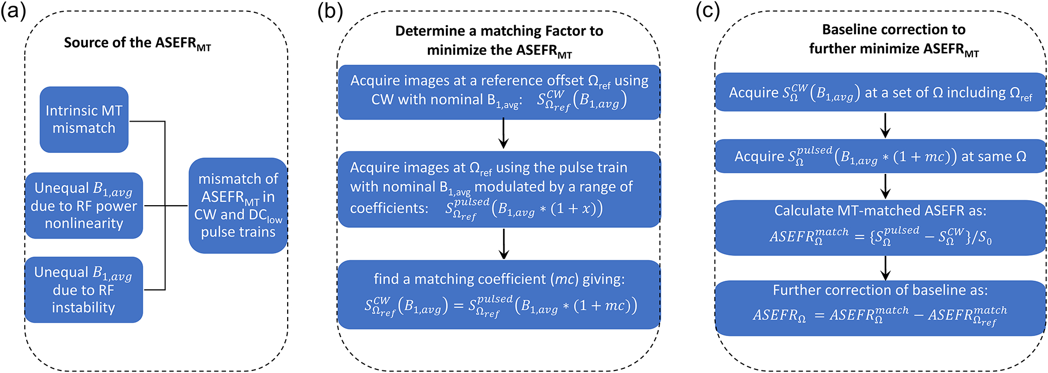
(A) The mismatch in observed baseline MT effect between signals saturated by high and low DC pulse trains may have three contributions: the intrinsic MT mismatch, and mismatch in the actual B_1,avg in the two pulse trains due to the nonlinearity and instability in the applied RF power. (B) The baseline MT mismatch can be mitigated by employing a matching procedure to determine a matching coefficient (mc) to adjust the power of the low DC pulse train so that the MT effects of the CW pulse and low DC pulse trains are matched at a reference frequency (Ω_ref) with minimal CEST effect. (C) Additionally, a baseline correction can be used to rectify any residual signal that may result from disparate MT effects across the ASEFR image.

In this study, we investigated the mismatch between the MT effect under high and low duty cycle pulse trains within the context of ASEF imaging, where an empirical correction procedure was used in ensuring proper MT filtering and compensate for the baseline MT mismatch. We first evaluated the effects of average saturation power and semi-solid pool MT fraction on the matching coefficient (mc) using Nicotinamide phantoms in heat denatured BSA. We then examined the matching coefficient measurement, the baseline MT signal, and the contrast of ASEF imaging of stroke rats induced by Middle Cerebral Artery Occlusion (MCAO) to evaluate the potential of ASEF imaging in vivo.

Methods

Simulations

CEST signals were simulated by Bloch-McConnel Equations which include 3 exchanging pools of free water protons, labile protons, and bound water protons; the lineshape of the bound water was modeled by a super-Lorentzian function centered at −2.5 ppm. To separately evaluate the effect of each parameter, one of the following parameters was typically varied while keeping other parameters at the default value. We assumed a default bound water proton fraction (f_MT) of 0.08, a magnetization transfer rate between bound water and free water (k_MT) of 30 s⁻¹, a chemical shift between the labile proton and water of 3.5 ppm, a fraction of labile proton of 0.003 and a chemical exchange rate of 150 s⁻¹. The default T₁ (T₂) of water, labile proton, and bound water protons were assumed to be 2 s (66.6 ms), 2 s (66.6 ms), and 2 s (10 μs), respectively, and a default DC_low = 15% and bipolar pair duration of 24 ms was used (i.e., 12 ms for a single pulse). As an example of the ischemic tissue, the chemical exchange rate, k_MT and the T₂ of the bound water protons as assumed to be 60 s⁻¹, 20 s⁻¹ and 15 μs, respectively.

MRI Experiments

All MR experiments were performed on a Bruker Biospec 9.4 T magnet (Billerica, MA, USA). The magnetic field homogeneity was optimized by localized shimming over the volume of interest. The CEST pulse sequence consists of saturation preparation module followed by spin-echo echo planar imaging (EPI). Saturation preparation schemes consisted of either a single CW block pulse or a train of binomial pairs of Gaussian pulses with a kurtosis of 4⁴¹. While MTR_asym is commonly used as a convenient measure of the CEST signal, it has recently been established that asymmetry analysis introduces contaminations from the MTC asymmetry of the semisolid macromolecules and the NOE effect which could be larger than the CEST signal of interest^13,19,30,36. Thus, only positive RF frequencies were acquired in this study. To achieve a relative higher sensitivity for ASEF, a larger difference in DC is needed for the two pulse trains. On the other hand, a larger DC difference will lead to larger baseline MT mismatch which would be more difficult to correct⁴¹. Thus, to balance these two needs, in this work a CW pulse was chosen which has a maximal DC of 1, and a duty cycle of 15% was selected for the low DC pulse train.

Phantom Experiments

A set of four phantoms were prepared in 1× phosphate buffered saline (PBS). 12% (w/v) Bovine Serum Albumin (BSA), 10% BSA with 150 mM Nicotinamide (Nic), 12% BSA with 150 mM Nic, and 15% (w/v) BSA with 150 mM Nic were prepared and titrated to pH of 7.4. These phantoms were then transferred into syringes, heated in a water bath at 95°C for 20 minutes to denature the BSA within the phantoms, and allowed to cool before imaging at room temperature.

Imaging was performed in a 4.0-cm inner-diameter volume coil used for excitation and reception with a 6-s saturation preparation. Average B₁ powers of 0.60, 0.72, 0.86, 1.03, 1.25, 1.50 and 1.80 μT were applied comprising either a single CW block pulse or a train of 37 binomial pairs with durations of 24 ms and pulse intervals of 138.1 ms, yielding a duty cycle (DC) of about 15%. For each of these powers, a total of 26 RF offsets were acquired with a scanning time of 4.8 minutes. The imaging parameters for the single slice EPI read out were matrix size = 64 × 64, field of view = 50 × 50 mm, slice thickness = 5 mm, TR = 11 s and TE = 20 ms. T₁ mapping was performed with an inversion recovery EPI sequence. B₀ maps were obtained using the WASSR method⁴³ for region of interest (ROI) selection of pixels with a low B₀ inhomogeneity. B₁ mapping was obtained by measuring signal nutation as was performed in Vaughan et al⁴⁴.

In vivo Experiments

Six male Sprague-Dawley rats (253–351 g) were studied with the approval of the Institutional Animal Care and Use Committee at the University of Pittsburgh. The animals were anesthetized with isoflurane (5% for induction and 2% during surgery) in a mixture of O₂ and air gases maintaining total O₂ concentration at ~30% throughout the experiment. Prior to imaging, MCAO was performed to induce permanent ischemia in the left hemisphere. During imaging, isoflurane was reduced to 1.4–1.5% maintaining end-tidal CO₂ at 3–4%, while the rectal temperature was controlled at 37.2±0.5°C using a feedback-controlled heating pad.

Imaging was performed at 3–4 hours post-operation with an 86-mm inner-diameter volume coil for excitation and a 20-mm single loop coil for reception. A 4-s saturation preparation with average B₁ of 0.80 μT was applied at 36 offsets between 0 and 6 ppm in either a single 4-s CW block pulse or a train of 25 binomial pairs with durations of 24 ms and pulse intervals of 136 ms (DC_low = 15%). A control scan at 300 ppm was acquired with 5 averages for normalization, and the scan time is 4.75 minutes for each spectrum (9.5 min for both CW and low DC pulse train). The spectrum was measured for 4 repetitions, so the total scan time of ASEF spectra is 38 min. The two slice EPI readout was performed with the following imaging parameters: matrix size = 80 × 80, field of view = 32 × 32 mm, slice thickness = 2 mm, TR = 7 s and TE = 20 ms. To detect the ischemic lesion, ADC maps were acquired using a spin-echo EPI sequence, with a low b-value of 5 s/mm² applied on a single axis and high b-value of 1200 s/mm² applied along six different directions.

Background MT Matching using a matching coefficient

To compensate for the disparity of attenuation between the CW and the pulse train caused by machine limitations and the intrinsic difference in background MT, an empirical matching coefficient was determined as a scalar for the amplitude of RF irradiation in order to match the MT effects at an offset with minimal CEST effect (Fig. 1B). For this matching, baseline signals were measured at a reference frequency (i.e., Ω_ref = 5.5 ppm) using both the CW and the binomial pair pulse train. The nominal power of the CW pulse was fixed to B_1,avg while the average nominal power of the binomial pair pulse train was modulated around B_1,avg. An ROI was then drawn in the 12% BSA only phantom, or the normal tissue contralateral to the ischemic lesion in vivo, and the averaged signal in the ROI for the pulse train was linearly interpolated to determine the matching coefficient that achieves equality with the ROI averaged signal of the CW saturation scheme, i.e.,

$$S_{{\Omega }_{ref}}^{CW}\left(B_{1,avg}\right)=S_{{\Omega }_{ref}}^{\mathit{\text{pulsed}}}\left(B_{1,avg}*\left(1+mf\right)\right)$$ [1]

where Ω is the frequency offset. Assuming that with the same nominal B_1,avg, there is an imbalance in the actual B_1,avg of the two irradiation schemes due to the imperfection of the RF pulses:

$$B_{1,avg}^{CW}=B_{1,avg}^{\mathit{\text{pulsed}}}*\left(1+\eta \right)$$ [2]

The mc will compensate the mismatch due to both RF-imperfection and the intrinsic MT (when η = 0). Because η is dependent on the hardware and experimental setting, an initial matching can be performed with a wide range of mc variation (e.g., −25% to 25%) to determine a rough mc value, which can be obtained in a single pilot experiment. Then, more accurate matching can be performed with finer steps for all studies with similar experimental settings. For example, for the finer MT-matching of the in vivo experiments, the matching coefficient was varied between 1.5% to 12.5% in 19 uneven steps, i.e., increments of 0.4% for the middle 11 points and 0.9% for the outer 8 points.

Data Processing

All data were analyzed with in house developed Matlab code (MathWorks, Natick, Massachusetts, USA). For Z-spectra analyses, ROI were used. In phantoms, an ROI with minimal B₀ inhomogeneity (<0.05 ppm) was selected from each sample; while in MCAO animal studies, ROIs were drawn on ADC maps encompassing the entirety of the infarcted region and then reflected over the center of the brain to determine a region for the contralateral side. The Z-spectra and the numerical ASEFR values were obtained by first averaging over the ROIs in both imaged slices in each animal, and then the mean and standard deviation were calculated across all six animals. The MT-matched ASEFR was calculated from the difference between the CW and pulse train saturations as follows:

$${\mathit{\text{ASEFR}}}_{\Omega }^{\mathit{\text{match}}}=\raisebox{1ex}{$\left(S_{\Omega }^{\mathit{\text{pulsed}}}\left(B_{1,avg}*\left(1+mf\right)\right)-S_{\Omega }^{CW}\left(B_{1,avg}\right)\right)$}\!\left/ \!\raisebox{-1ex}{$S_0$}\right.$$ [3]

where S₀ images were acquired at 300 ppm. Even with the application of a matching coefficient, there may be residue MT mismatch due to B₁ inhomogeneity or tissue heterogeneity (such as the ischemic tissue). To further correct for this residue MT-mismatch, the ASEFR from the reference frequency of Ω_ref = 5.5 ppm were then subtracted from all offsets (Fig. 1C), i.e.,

$${\mathit{\text{ASEFR}}}_{\Omega }={\mathit{\text{ASEFR}}}_{\Omega }^{\mathit{\text{match}}}-{\mathit{\text{ASEFR}}}_{{\Omega }_{ref}}^{\mathit{\text{match}}}$$ [4]

To compare with the amide CEST imaging, 3-point estimation of APT was calculated as follows¹⁹: $\text{APT}*=[(S_{3.0\text{ppm}}^{CW}+S_{4.2\text{ppm}}^{CW})/2-S_{3.6\text{ppm}}^{CW}]/S_0$. Box and whisker plots were created to compare APT* and ASEFR at the offsets of 3.6 ppm, 2.0 ppm, and 2.6 ppm by determining the mean and quartile values for the mean of APT* and the ASEFR values at each of these offsets.

ASEFR is a sensitivity index which is coupled to other relaxation effects such as MT and the T₁ of water. For more specific analysis of the CEST signal, an exchange-dependent relaxation rate can be calculated as^45,46:

$$R_{ex, \mathit{\text{ASEF}}}\left(\Omega \right)=\left\{\frac{S_0}{S_{\Omega }^{CW}}-\frac{S_0}{S_{\Omega }^{\mathit{\text{pulsed}}}}\right\}·\frac{{\Omega }^2}{T_1 {\left(\gamma B_{1,avg}\right)}^2}$$ [5]

which can minimize these confounding relaxation effects and be applied to determine the exchange rate and the concentration of the labile proton of interest.

Results

Due to the exchange rate-filtering of the ASEF, the simulated Z-spectra of the CW and the DC_low pulse trains showed a clear difference at the CEST signal dip at 3.5 ppm (Fig. 2a). When the RF system is ideal and η = 0, there is a small difference of ~0.5% at the signal between 4–6.5 ppm due to the intrinsic MT mismatch. With an assumed RF imbalance of η = 6%, the signal difference becomes larger (>2%). The ASEFR signals obtained from the difference between the CW and DC_low Z-spectra show distinct CEST peaks at 3.5 ppm on top of broad baseline MT signals (Fig. 2b). A matching coefficient of 2.1% was determined at 5.5 ppm for the DC_low(η = 0) and 8.1% for the DC_low(η = 6%) pulse train, which minimized the ASEFR_MT signal for the normal tissue. However, small residue ASEFR_MT signals may exist for a few cases, such as for ischemic tissue with different MT properties (−0.2% at 5.5 ppm, blue, Fig. 2c), when there exist a B₁ inhomogeneity of 10% (−0.14% at 5.5 ppm, red), or there is 1% error in the measurement of the mc (+0.26% at 5.5 ppm, green). A baseline-correction using Eq. [4] minimized these residue ASEFR_MT signals, so that the CEST signal can be compared with relatively high specificity (Fig. 2d). Indeed, the CEST signal peak at 3.5 ppm for normal tissue is 3.14% and 3.08% for B_{1, avg} = 1 μT and 0.9 μT, and is 3.17% for B_{1, avg} = 1 μT with 1% error in the mf, respectively, indicating a satisfactory correction of the B₁ inhomogeneity and measurement error of mc.

Fig. 2.

Simulated Z-spectra and ASEFR spectra for B_1,avg = 1 μT demonstrating the explanatory procedures for correction of the baseline MT mismatch. (A) While the CEST signal dip at 3.5 ppm becomes much smaller with the DC_low pulse train than that of the CW pulse as expected from the exchange rate filtering, there is small intrinsic mismatch in the MT signal of normal tissue between the two saturation schemes with the same an actual B_1,avg (i.e., η = 0). For a DC_low pulse train with η=6%, the mismatch in the MT signal appears larger. Inset: enlarged signals in the 3 to 5.5 ppm range. (B) The raw ASEFR signals obtained from A without any correction shows a distinct CEST peak, on top of the broad MT baseline which is smaller with η =0 and is larger with η = 6%. (C) Using a matching coefficient determined at 5.5 ppm, the matched ASEFR spectrum minimizes the ASEFR_MT signal for normal tissue, but is less effective for the ASEFR_MT signal of pathological tissue (blue), when there is a B₁ inhomogeneity of 10% (red), or when there is a 1% error in the measurement of mc (green). (D). A baseline correction at 5.5 ppm can be performed to minimize the residue ASEFR_MT signals caused by the pathological tissue, B₁ inhomogeneity or small error in the mc measurement.

Fig. 3a showed the simulated intrinsic ASEFR_MT (in the case of η = 0) on B_{1, avg} for 3 RF offsets of 2, 3.5, and 5.5 ppm. The ${\mathit{\text{ASEFR}}}_{MT}^{raw}$ increases quadratically with B_{1, avg}, and is higher at 2 ppm than 3.5 and 5.5 ppm. The ${\mathit{\text{ASEFR}}}_{MT}^{raw}$ is also strongly affected by the DC of the pulse train and is much higher for a DC_low of 10% than those of 15% and 25%, as shown for 5.5 ppm in Fig. 3b. As such, the mc value determined at 5.5 ppm is also strongly affected by DC_low, and increases with B_1,avg (Fig. 3c). After the MT-matching process using mc, the ${\mathit{\text{ASEFR}}}_{MT}^{\mathit{\text{match}}}$ becomes zero for 5.5 ppm. While there are still residue signals for 3.5 ppm and 2.0 ppm, they are very small for low B_{1, avg} values (<0.25% for B_{1, avg} < 1 μT). To evaluate the dependence of mc on the MT properties, the mc value at 5.5 ppm were simulated for B_{1, avg} = 0.8 μT as a function of a few parameters of the semisolid macromolecule and the water pools. Fig. 4a and 4b showed that the mc is sensitive to the T₂ of the semisolid macromolecules and the magnetization transfer rate, respectively. In contrast, the mc is only weakly affected by the MT pool size (Fig. 4c), and the T₁ (Fig. 4d) and T₂ (Fig. 4e) of the water pool.

Fig. 3.

Simulated dependence of the intrinsic ASEFR_MT and the matching coefficient on B_1,avg, assuming that the actual B_1,avg is equal for DC_low and CW (i.e., η = 0). (A) Raw ASEFR_MT signal increases almost quadratically with B_1,avg, and is larger at 2 ppm than that of 3.5 ppm and 5.5 ppm. Both (B) Raw ASEFR_MT signal and (C) the mc at 5.5 ppm are strongly affected by DC_low. (D) With the application of mc for the DC_low pulse train at 5.5 ppm, the ASEFR_MT^match signal is minimized at 5.5 ppm. While there is still residue ASEFR_MT^match signals at 3.5 ppm and 2 ppm, the residue ASEFR_MT^match signals are small for small power of B_1,avg < 1 μT.

Fig. 4.

Simulated dependence of matching coefficient (mc) on the parameters of the MT and water pools, assuming that the actual B_1,avg is equal for DC_low and CW. The matching coefficient shows strong dependence on the T₂ of the semisolid macromolecule proton (A) and the magnetization transfer rate (B), whereas the dependence is much weaker on the (C) MT pool size, and on the (D) T₁ and (E) T₂ of the water pool.

Fig. 5a shows an example of matching coefficient determination at a B_1,avg of 0.86 μT for the Nicotinamide phantoms at 5.5 ppm. The CW pulse is imaged at a fixed power of 0.86 μT (data points indicated by ‘*’ at mc = 0). A higher concentration of denatured BSA have larger MT pool fraction resulting in lower attenuated signal levels, whereas increasing the matching coefficients for the binomial pulse train leads to increasing attenuation. Linear interpolation (solid fitting line) was used to determine the matching coefficient value at which the attenuation from the CW pulse (the average value indicated by the dotted straight line) is approximately equivalent to that of the pulse train. There was little difference in the matching coefficients of the 4 phantoms despite the 50% increase in BSA concentration contributing to the background MT. In Fig. S1 of the supplementary information, the map of mc for B_{1, avg} = 0.86 μT showed very small difference across these phantoms. On the other hand, matching coefficient increased almost linearly with increasing power (Fig. 5b), in good agreement with the simulation of Fig. 4c and 3c, respectively. Fig. 5c shows the residual raw ASEFR at 5.5 ppm. Since the matching coefficient determination was performed at this frequency, most of the data points are within 0.3% of a zero baseline. As there may be variation across the image (e.g., caused by B₁-inhomogeneity), baseline correction is used to further suppress the ASEFR_MT and improve the specificity of the CEST signal (Fig. 5c). The CEST signal of the Nicotinamide phantoms as measured by ASEF at the amide frequency of 3.4 ppm (Fig. 5d) was lower for increasing BSA content because of their larger MT effect and shorter T₁ values. When the R_{ex, ASEF} is calculated for the ASEF signal using Eq. [5], the MT and T₁ effects were suppressed, so that the R_{ex, ASEF} values became very close for all 3 phantoms with Nic. As shown in Supporting Information Figure S1, clear difference were observed among the Nic phantoms in the ASEFR map at 3.4 ppm for B_{1, avg} = 0.86 μT, but diminished in the R_{ex, ASEF} map. The residual signal for the phantom without Nicotinamide is small, especially at lower B_1,avg where the background residual signal is removed more effectively.

Fig. 5. Saturation Power and MT dependency of the matching coefficient and raw ASEFR signals at baseline and on resonance for Nicotinamide (Nic) phantoms in denatured BSA.

(A) Example of matching procedure acquiring CW signals at a fixed power (* at mc = 0) while acquiring 15% DC pulse train signals at modulating B_1,avg (circle) to determine the matching coefficient at which average value of the CW (dotted line) crosses the fit of the pulse train (solid line) for phantoms with 12% denatured BSA alone (black), 150 mM Nic in 10% denatured BSA (red), 150 mM Nic in 12% denatured BSA (green), and 150 mM Nic in 15% denatured BSA (blue). (B) Matching coefficients are similar across each phantom but varies with power (fit shown by solid line). (C) With the applied mc, the MT-matched ASEFR signals (ASEFR^match) of the four phantoms at baseline offset of 5.5 ppm as a function of B_1,avg. (D) A voxel-wise correction at the baseline offset of 5.5 ppm was used to obtain the ASEFR signals of the four phantoms on the amide resonance of 3.4 ppm as a function of B_1,avg. (E) R_ex obtained from the ASEF data are close for all the Nic phantoms. Error bars in B, C, D, E: voxel-wise standard deviation.

In Figure 6, we examine the matching coefficient measurement in vivo in an MCAO rat model. The lesions are visible in the left hemisphere of the ADC maps as a ~30% decrease in ADC (Fig. 6a). An ROI was selected from the lesion (red outline) and the contralateral tissue (blue outline). The matching coefficient maps calculated across the rat brain show some disparity between the lesion and the normal tissue. The B_1,avg maps show the B₁-inhomogeneity has a magnitude of several percent, and is mainly in the vertical direction, suggesting that the differences in matching coefficients between ischemic and normal tissue are not due to differences in B₁. Baseline MT-matching across these ROIs (Fig. 6b) was performed similar to the phantom study in Fig. 5. In this representative animal, the results averaged from the ROIs of the 2 slices show a slightly lower matching coefficient for the lesion (4.9%, black data) than for the contralateral ROI (7.2%, red data). A box plot of the matching coefficients in the lesion and contralateral ROI shows an ~1.3% difference in the averaged values (6.0% for lesion and 7.3% for contralateral regions, n = 6), but there is a wider spread of values and inter-animal variation in the lesion, compared to the matching coefficient of the contralateral (Fig. 6c). This variability and heterogeneity suggest that the matching coefficient likely varies with the MT properties of the ischemic tissue, as expected from the simulation results in Fig. 4. Therefore, the matching coefficients for the contralateral side were used for acquisition of ASEF in vivo for better consistency.

Fig. 6. ADC and Matching coefficient maps, example matching and comparison of healthy and infarcted tissue of MCAO rodents.

(A) ADC, matching coefficient, and B₁ maps of an exemplary MCAO rodent across two slices (lesion ROI indicated by red and contralesional ROI indicated by blue). (B) Matching procedure in an exemplary MCAO rodent shows different matching coefficients for the lesion and contralesional tissues. (C) Box and whisker plot of the matching coefficients calculated for lesion and contralesional tissue across MCAO rodents (n = 6).

For the contralateral ROI, the positive offsets of the Z-spectra averaged over animals (Fig. 7a) show close matching between the CW saturated spectra and the low duty cycle pulsed spectra in offsets beyond chemical exchange resonances (e.g., >5 ppm). In contrast, there is a clear disparity between the CW and pulsed spectra around 1.5 to 4 ppm particularly around ~3.6 ppm, ~2 ppm, and the 2.6 ppm frequencies, indicating that the low DC pulse train effectively reduced these CEST signals. In the lesion ROI, there is a small mismatch at large offsets (>5 ppm) for the average Z-spectra (Fig. 7b) as the mc determined by baseline MT-matching was taken from the contralateral ROI. Subtracting the CW from the pulsed spectra gives a ASEFR^match spectra for the lesion and contralateral tissue (Fig. 7c). Examining the ASEFR^match spectra shows disparate baselines around 5.5 ppm and observing the spectra closer over 5–6 ppm shows that the average baseline for the contralateral ROI is close to zero but is about −0.3% for the lesion ROI. Subtracting this 5.5 ppm baseline across voxels from the whole ASEFR^match spectra gives corrected spectra for both the contralateral as well as the lesion (Fig. 7d). The ASEFR for the amide resonance at 3.6 ppm was about 2.9% for the tissue contralateral to the lesion, whereas in the lesion it measured an average of 1.6%. At 2 ppm, the contralateral side displayed an average guanidyl-weighted signal of 2.3% while the lesion exhibited a signal of 2.2%. At 2.6 ppm, while the CEST signal peak was difficult to discern from the CW spectra alone, the ASEF measurement exhibits a small peak with a magnitude of about 1.9% for the contralateral tissue and 1.1% in the ischemic region.

Fig. 7. Z-spectra and the ASEFR spectra of MCAO rodents.

(A) Average Z-spectra acquired using saturation by CW (black) and 15% DC pulse trains (red) in healthy contralesional tissue in MCAO rodents. (B) Average Z-spectra acquired using saturation by CW (black) and 15% DC pulse trains (red) in infarcted lesion tissue in MCAO rodents. (C) Average raw ASEFR calculated from the difference between signal saturated by 15% DC pulse trains and CW in lesion (black) and contralesional tissue (red). (D) Baseline-corrected ASEFR in lesion (black) and contralesional tissue (red).

The sensitivity of the ASEF technique at the amide frequency, ASEFR_{3.6 ppm}, was compared to the APT*. In Figure 8a and 8b, both APT* and the ASEFR_{3.6 ppm} show good contrast between the ischemic and the healthy tissue for the two representative animals, and the lesion location are in good agreement with those of the ADC deficit regions. Figure S2 of Supporting Information showed these results for all 6 animals. Boxplots of both metrics (Fig. 8c) show a similar breadth in the range of values for the ischemic lesion, while APT* shows a much tighter distribution of values across animals for the normal tissue. APT* averaged over the lesion was 1.21 ± 0.4% and 2.43 ± 0.1% for the contralateral tissue, while ASEFR_{3.6 ppm} measured 1.6 ± 0.4% in the lesion and 2.9 ± 0.4% in the contralateral hemisphere. Comparatively, ASEFR_{3.6 ppm} shows higher magnitude than APT* in both the healthy tissue as well as the ischemic lesion, but the contrast between the two types of tissues is nearly equal, being 1.22 ± 0.38% for APT* and 1.3 ± 0.52% (n = 6) for ASEFR_{3.6 ppm}.

Fig. 8. Comparison of APT* and ASEFR at 3.6 ppm in MCAO rodents.

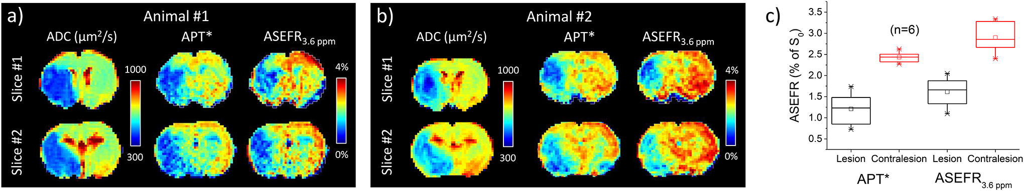
(A,B) ADC, APT* and 3.6 ppm ASEFR maps of two exemplary MCAO rodents across two slices. (C) Box and whisker plot of the average APT* and ASEFR at 3.6 ppm in the lesion (black) and contralesional tissue (red). The data were averaged over the ROIs obtained from two slices, and then averaged over 6 rats.

The ASEFR signals at the resonance of 2.0 ppm and 2.6 ppm were further examined in Figure 9. The representative maps (Fig. 9a and 9b) showed spatial inhomogeneity (particularly within the ischemic lesion) for ASEFR_{2 ppm}, but the overall contrast between the lesion and the contralateral region is low. The ASEFR_{2.6 ppm}, on the other hand, showed strong contrast between the lesion and the contralateral tissue. Similar results were observed from other animals, as shown in Supporting Information Fig. S3. Despite the spatial inhomogeneity, ASEFR_{2 ppm} signals averaged over the lesion and contralateral tissue are similar (Fig. 9c). The ASEFR_{2.6 ppm} showed a drop in the lesion as compared to the contralateral tissue resembling the drop in ASEFR_{3.6 ppm}, though the contrast of ASEFR_{2.6 ppm} is about 40% smaller than that of ASEFR_{3.6 ppm} (0.8% versus 1.3%).

Fig. 9. Comparison of ASEFR at 2.0 ppm and 2.6 ppm in MCAO rodents.

(A,B) 2.0 and 2.6 ppm ASEFR maps of two exemplary MCAO rodents across two slices. (C) Box and whisker plot of the average ASEFR at 2.0 and 2.6 ppm in the lesion (black) and contralesional tissue (red).

Discussion

We have examined practical considerations in implementing ASEF for CEST MRI, and demonstrated the feasibility of ASEF imaging in vivo. To minimize the mismatch of the MT effect in the ASEF signal, two steps are taken: 1) a matching coefficient was calibrated at a reference frequency to provide a 1^st order matching of the MT attenuation of the CW and the low DC pulse train, and 2) a baseline correction was made using the ASEFR measured at the reference frequency. Our results show that ASEF imaging can probe various labile protons of interest which may include amide, PCr, and guanidyl groups. Compared to model-fitting methods such as Lorentzian fitting, the acquisition time burden for ASEF is significantly lessened. When compared to APT*, ASEFR_{3.6 ppm} exhibited higher signal magnitude but also higher inter-animal variability (a standard deviation of 0.4% in the contralesional tissue compared to 0.1% for APT*). Although it does not provide an advantage in the contrast to noise ratio, ASEF can be applied to conditions where methods like 3-point measurement and PLOF are hard to implement due to the lack of a distinct peak, such as at lower magnetic fields.

In this pilot in vivo study, three potential contrasts were demonstrated at 3.6, 2.6, and 2.0 ppm with a single set of ASEF parameters. Since ASEF contrast is sensitive to parameters such as B_1,avg and difference in the duty cycle of the two pulse trains, ASEF parameters could be optimized individually to improve the sensitivity of each CEST signal obtained. For example, the optimal amide CEST signal at 3.6 ppm was reported to be about 1 μT for 9.4 T¹⁹ or 2 μT for 3 T⁴⁷, whereas optimal PCr-weighted CEST signals at 2.6 ppm was reported to be only around 0.5 to 0.7 μT³¹. Note that the signal for 2.6 ppm (~1.9 % in the contralateral tissue) reported here is higher than what we might expect from brain PCr alone (<1%), indicating there may be other sources of contrast in ASEFR_{2.6 ppm}, such as the amide from protein sidechains, amine protons with a close resonance frequency, and slow NOE signal from aromatic protons⁴⁸. Besides B_1,avg, the DC of the pulse train may also be adjusted to improve the sensitivity of these CEST signals. However, because the MT-mismatch and the matching coefficients are highly sensitive to B_1,avg and the DC of the pulse train (Fig. 3b and 3c), a lower B_1,avg and higher DC_low would be preferred to reduce the MT-mismatch.

CEST signal at 2 ppm is dominated by guanidyl water proton exchange, and the power of 0.8 μT is likely suboptimal for normal physiological conditions with a relatively fast exchange rate of ~1000 s^{−1 49,50}. The near-zero contrast between the ischemic and normal tissue can be explained by the B₁-tuning effect⁴, as previous studies have reported a positive ischemic contrast with lower B₁ power level, and a negative contrast at a higher power level⁴. Because the exchange rate filtering domain of ASEF is determined by B_1,avg⁴¹, an adjustment of B_1,avg to either a lower or higher value may change the ischemic contrast. While the simple subtracted signal for ASEF was primarily used in this study for sensitivity comparison, ASEF signals can readily be converted into relaxation rate related indices (e.g., R_ex, as shown in Fig. 4)^46,51 which is a more specific measure and can potentially be converted to quantitative physiological information such as metabolite concentration and/or tissue pH. Note that in the phantom study, non-negligible residual ASEFR signal of 0.5 to 1.5% was observed at 3.4 ppm in Fig. 5d, which is 4–7 times larger than the simulated value in Fig. 3d. This is different with our recent study, where the ASEFR MT signal is effectively minimized in agar phantoms⁴¹. Thus, we postulate that the proteins were not completely immobilized in the heated-BSA samples, and there may exist a very small amount of BSA with limited mobility and detectable CEST or aromatic NOE effect. This small amount of BSA may have contributed to the majority of the residue ASEFR signal at 3.4 ppm.

While important in reducing the background MT signal for ASEFR, the matching of the MT effect between the CW and pulsed trains using a matching coefficient likely introduced an additional factor of variability. Disparate MT effects are also observed in techniques such as VDMP, which may be matched by modulating the difference in mixing time⁴⁰. Our MCAO results showed a clear disparity between matching coefficient in healthy and ischemic tissue. As shown in the simulation of Fig. 4, this disparity may be because that the ASEF signal from the MT background can vary with tissue properties such as the magnetization transfer rate and the T₂ of the semi-solid pool⁴¹. Because the MT mismatch may not be fully minimized by a single matching coefficient, we have additionally employed a baseline correction at 5.5 ppm to suppress the residual difference, which can also correct small residue MT-mismatch caused by B₁ inhomogeneity or error in the measurement of mc. The results in Fig. 3d and 7c indicate that the baseline ASEFR is slightly dependent on the RF offset, therefore, a reference frequency must maintain minimal CEST effect yet be as close as possible to the resonance frequency of the labile proton of interest to provide the best suppression of the background signal.

Beside the intrinsic MT mismatch, other possible sources of background ASEFR signal may be due to hardware imperfectness, including RF power linearity and stability during a long saturation duration. In our in vivo experiments with a relatively low B_1,avg of ~0.8 μT, the intrinsic MT-mismatch is expected to be small according to the simulation results. Thus, we postulate that the major contribution to our baseline ASEFR_MT signal and to the mc value (~7%) is the hardware imperfection. These issues will more likely be site-dependent, and hardware improvement such as parallel RF transmission may reinforce dependability in power deposition. For experiments with similar settings (e.g., coil, weight of the subject), the matching coefficient is expected to be similar, so the matching coefficient measurement may be performed just once during the pilot study to save acquisition time. Indeed, our simulation showed that an error of the mc on the order of 1% can be satisfactory corrected by the baseline-correction using Eq. [4]. In other words, standardizing the matching coefficient, and relying more on the baseline correction could reduce the burden on acquisition time with limited effect on the accuracy of ASEFR.

Conclusions

CEST imaging with ASEF can suppress fast exchanges and semi-solid MT background with only small loss to sensitivity. It can probe slow exchange species such as amide, guanidyl and PCr groups and can be applied to the study of stroke, tumor, muscle pathology, etc. Its low requirement on number of imaged signals also opens up possibilities for dynamic imaging. ASEF can be easily adapted to the standard CEST imaging pulse sequence which allows for seamless integration of a myriad of techniques currently being developed in the CEST field.

References

- 1.Ward KM, Aletras AH, Balaban RS. A new class of contrast agents for MRI based on proton chemical exchange dependent saturation transfer (CEST). J Magn Reson. 2000;143(1):79–87. [DOI] [PubMed] [Google Scholar]
- 2.Chen LQ, Howison CM, Jeffery JJ, Robey IF, Kuo PH, Pagel MD. Evaluations of extracellular pH within in vivo tumors using acidoCEST MRI. Magn Reson Med. 2014;72(5):1408–1417. [DOI] [PMC free article] [PubMed] [Google Scholar]
- 3.Guo Y, Zhou IY, Chan ST, et al. pH-sensitive MRI demarcates graded tissue acidification during acute stroke - pH specificity enhancement with magnetization transfer and relaxation-normalized amide proton transfer (APT) MRI. Neuroimage. 2016;141:242–249. [DOI] [PMC free article] [PubMed] [Google Scholar]
- 4.Jin T, Wang P, Hitchens TK, Kim SG. Enhancing sensitivity of pH-weighted MRI with combination of amide and guanidyl CEST. Neuroimage. 2017;157:341–350. [DOI] [PMC free article] [PubMed] [Google Scholar]
- 5.Longo DL, Dastru W, Digilio G, et al. Iopamidol as a responsive MRI-chemical exchange saturation transfer contrast agent for pH mapping of kidneys: In vivo studies in mice at 7 T. Magn Reson Med. 2011;65(1):202–211. [DOI] [PubMed] [Google Scholar]
- 6.Sun PZ, Cheung JS, Wang E, Lo EH. Association between pH-weighted endogenous amide proton chemical exchange saturation transfer MRI and tissue lactic acidosis during acute ischemic stroke. J Cereb Blood Flow Metab. 2011;31(8):1743–1750. [DOI] [PMC free article] [PubMed] [Google Scholar]
- 7.Sun PZ, Longo DL, Hu W, Xiao G, Wu R. Quantification of iopamidol multi-site chemical exchange properties for ratiometric chemical exchange saturation transfer (CEST) imaging of pH. Phys Med Biol. 2014;59(16):4493–4504. [DOI] [PMC free article] [PubMed] [Google Scholar]
- 8.Sun PZ, Wang E, Cheung JS, Zhang X, Benner T, Sorensen AG. Simulation and optimization of pulsed radio frequency irradiation scheme for chemical exchange saturation transfer (CEST) MRI-demonstration of pH-weighted pulsed-amide proton CEST MRI in an animal model of acute cerebral ischemia. Magn Reson Med. 2011;66(4):1042–1048. [DOI] [PMC free article] [PubMed] [Google Scholar]
- 9.Zhou J, Payen JF, Wilson DA, Traystman RJ, van Zijl PC. Using the amide proton signals of intracellular proteins and peptides to detect pH effects in MRI. Nat Med. 2003;9(8):1085–1090. [DOI] [PubMed] [Google Scholar]
- 10.Xu X, Chan KW, Knutsson L, et al. Dynamic glucose enhanced (DGE) MRI for combined imaging of blood-brain barrier break down and increased blood volume in brain cancer. Magn Reson Med. 2015;74(6):1556–1563. [DOI] [PMC free article] [PubMed] [Google Scholar]
- 11.Zaiss M, Anemone A, Goerke S, et al. Quantification of hydroxyl exchange of D-Glucose at physiological conditions for optimization of glucoCEST MRI at 3, 7 and 9.4 Tesla. NMR Biomed. 2019;32(9):e4113. [DOI] [PMC free article] [PubMed] [Google Scholar]
- 12.Zhou J, Lal B, Wilson DA, Laterra J, van Zijl PC. Amide proton transfer (APT) contrast for imaging of brain tumors. Magn Reson Med. 2003;50(6):1120–1126. [DOI] [PubMed] [Google Scholar]
- 13.Zu Z, Xu J, Li H, et al. Imaging amide proton transfer and nuclear overhauser enhancement using chemical exchange rotation transfer (CERT). Magn Reson Med. 2014;72(2):471–476. [DOI] [PMC free article] [PubMed] [Google Scholar]
- 14.Chan KW, McMahon MT, Kato Y, et al. Natural D-glucose as a biodegradable MRI contrast agent for detecting cancer. Magn Reson Med. 2012;68(6):1764–1773. [DOI] [PMC free article] [PubMed] [Google Scholar]
- 15.Desmond KL, Moosvi F, Stanisz GJ. Mapping of amide, amine, and aliphatic peaks in the CEST spectra of murine xenografts at 7 T. Magn Reson Med. 2014;71(5):1841–1853. [DOI] [PubMed] [Google Scholar]
- 16.Heo HY, Zhang Y, Jiang S, Lee DH, Zhou J. Quantitative assessment of amide proton transfer (APT) and nuclear overhauser enhancement (NOE) imaging with extrapolated semisolid magnetization transfer reference (EMR) signals: II. Comparison of three EMR models and application to human brain glioma at 3 Tesla. Magn Reson Med. 2016;75(4):1630–1639. [DOI] [PMC free article] [PubMed] [Google Scholar]
- 17.Jin T, Iordanova B, Hitchens TK, et al. Chemical exchange-sensitive spin-lock (CESL) MRI of glucose and analogs in brain tumors. Magn Reson Med. 2018;80(2):488–495. [DOI] [PMC free article] [PubMed] [Google Scholar]
- 18.Zhou J, Tryggestad E, Wen Z, et al. Differentiation between glioma and radiation necrosis using molecular magnetic resonance imaging of endogenous proteins and peptides. Nat Med. 2011;17(1):130–134. [DOI] [PMC free article] [PubMed] [Google Scholar]
- 19.Jin T, Wang P, Zong X, Kim SG. MR imaging of the amide-proton transfer effect and the pH-insensitive nuclear overhauser effect at 9.4 T. Magn Reson Med. 2013;69(3):760–770. [DOI] [PMC free article] [PubMed] [Google Scholar]
- 20.Jin T, Wang P, Zong X, Kim SG. Magnetic resonance imaging of the Amine-Proton EXchange (APEX) dependent contrast. Neuroimage. 2012;59(2):1218–1227. [DOI] [PMC free article] [PubMed] [Google Scholar]
- 21.Zong X, Wang P, Kim SG, Jin T. Sensitivity and source of amine-proton exchange and amide-proton transfer magnetic resonance imaging in cerebral ischemia. Magn Reson Med. 2014;71(1):118–132. [DOI] [PMC free article] [PubMed] [Google Scholar]
- 22.Sun PZ, Zhou J, Sun W, Huang J, van Zijl PC. Detection of the ischemic penumbra using pH-weighted MRI. J Cereb Blood Flow Metab. 2007;27(6):1129–1136. [DOI] [PubMed] [Google Scholar]
- 23.Chen L, Wei Z, Chan KWY, et al. Protein aggregation linked to Alzheimer’s disease revealed by saturation transfer MRI. Neuroimage. 2019;188:380–390. [DOI] [PMC free article] [PubMed] [Google Scholar]
- 24.Haris M, Cai K, Singh A, Hariharan H, Reddy R. In vivo mapping of brain myo-inositol. Neuroimage. 2011;54(3):2079–2085. [DOI] [PMC free article] [PubMed] [Google Scholar]
- 25.Haris M, Singh A, Cai K, et al. MICEST: a potential tool for non-invasive detection of molecular changes in Alzheimer’s disease. J Neurosci Methods. 2013;212(1):87–93. [DOI] [PMC free article] [PubMed] [Google Scholar]
- 26.Longo DL, Busato A, Lanzardo S, Antico F, Aime S. Imaging the pH evolution of an acute kidney injury model by means of iopamidol, a MRI-CEST pH-responsive contrast agent. Magn Reson Med. 2013;70(3):859–864. [DOI] [PubMed] [Google Scholar]
- 27.Pavuluri K, Manoli I, Pass A, et al. Noninvasive monitoring of chronic kidney disease using pH and perfusion imaging. Sci Adv. 2019;5(8):eaaw8357. [DOI] [PMC free article] [PubMed] [Google Scholar]
- 28.Vinogradov E, He H, Lubag A, Balschi JA, Sherry AD, Lenkinski RE. MRI detection of paramagnetic chemical exchange effects in mice kidneys in vivo. Magn Reson Med. 2007;58(4):650–655. [DOI] [PubMed] [Google Scholar]
- 29.Wu Y, Zhou IY, Igarashi T, Longo DL, Aime S, Sun PZ. A generalized ratiometric chemical exchange saturation transfer (CEST) MRI approach for mapping renal pH using iopamidol. Magn Reson Med. 2018;79(3):1553–1558. [DOI] [PMC free article] [PubMed] [Google Scholar]
- 30.Chen L, Barker PB, Weiss RG, van Zijl PCM, Xu J. Creatine and phosphocreatine mapping of mouse skeletal muscle by a polynomial and Lorentzian line-shape fitting CEST method. Magn Reson Med. 2019;81(1):69–78. [DOI] [PMC free article] [PubMed] [Google Scholar]
- 31.Chung JJ, Jin T, Lee JH, Kim SG. Chemical exchange saturation transfer imaging of phosphocreatine in the muscle. Magn Reson Med. 2019;81(6):3476–3487. [DOI] [PMC free article] [PubMed] [Google Scholar]
- 32.Rerich E, Zaiss M, Korzowski A, Ladd ME, Bachert P. Relaxation-compensated CEST-MRI at 7 T for mapping of creatine content and pH--preliminary application in human muscle tissue in vivo. NMR Biomed. 2015;28(11):1402–1412. [DOI] [PubMed] [Google Scholar]
- 33.Varma G, Girard OM, McHinda S, et al. Low duty-cycle pulsed irradiation reduces magnetization transfer and increases the inhomogeneous magnetization transfer effect. J Magn Reson. 2018;296:60–71. [DOI] [PubMed] [Google Scholar]
- 34.Haris M, Nanga RP, Singh A, et al. Exchange rates of creatine kinase metabolites: feasibility of imaging creatine by chemical exchange saturation transfer MRI. NMR Biomed. 2012;25(11):1305–1309. [DOI] [PMC free article] [PubMed] [Google Scholar]
- 35.Guivel-Scharen V, Sinnwell T, Wolff SD, Balaban RS. Detection of proton chemical exchange between metabolites and water in biological tissues. J Magn Reson. 1998;133(1):36–45. [DOI] [PubMed] [Google Scholar]
- 36.Hua J, Jones CK, Blakeley J, Smith SA, van Zijl PC, Zhou J. Quantitative description of the asymmetry in magnetization transfer effects around the water resonance in the human brain. Magn Reson Med. 2007;58(4):786–793. [DOI] [PMC free article] [PubMed] [Google Scholar]
- 37.Zaiss M, Schmitt B, Bachert P. Quantitative separation of CEST effect from magnetization transfer and spillover effects by Lorentzian-line-fit analysis of z-spectra. J Magn Reson. 2011;211(2):149–155. [DOI] [PubMed] [Google Scholar]
- 38.Lin EC, Li H, Zu Z, et al. Chemical exchange rotation transfer (CERT) on human brain at 3 Tesla. Magn Reson Med. 2018;80(6):2609–2617. [DOI] [PMC free article] [PubMed] [Google Scholar]
- 39.Zu Z, Louie EA, Lin EC, et al. Chemical exchange rotation transfer imaging of intermediate-exchanging amines at 2 ppm. NMR Biomed. 2017;30(10). [DOI] [PMC free article] [PubMed] [Google Scholar]
- 40.Xu X, Yadav NN, Zeng H, et al. Magnetization transfer contrast-suppressed imaging of amide proton transfer and relayed nuclear overhauser enhancement chemical exchange saturation transfer effects in the human brain at 7T. Magn Reson Med. 2016;75(1):88–96. [DOI] [PMC free article] [PubMed] [Google Scholar]
- 41.Jin T, Chung JJ. Average Saturation Efficiency Filter (ASEF) for CEST Imaging. Magn Reson Med. 2022; DOI: 10.1002/mrm.29211. [DOI] [PMC free article] [PubMed] [Google Scholar]
- 42.Hua J, Hurst GC. Analysis of on- and off-resonance magnetization transfer techniques. J Magn Reson Imaging. 1995;5(1):113–120. [DOI] [PubMed] [Google Scholar]
- 43.Kim M, Gillen J, Landman BA, Zhou J, van Zijl PC. Water saturation shift referencing (WASSR) for chemical exchange saturation transfer (CEST) experiments. Magn Reson Med. 2009;61(6):1441–1450. [DOI] [PMC free article] [PubMed] [Google Scholar]
- 44.Vaughan JT, Garwood M, Collins CM, et al. 7T vs. 4T: RF power, homogeneity, and signal-to-noise comparison in head images. Magn Reson Med. 2001;46(1):24–30. [DOI] [PubMed] [Google Scholar]
- 45.Chung JJ, Jin T. Low duty cycle pulse trains for exchange rate insensitive chemical exchange saturation transfer MRI. Magn Reson Med. 2021;86(5):2542–2551. [DOI] [PMC free article] [PubMed] [Google Scholar]
- 46.Jin T, Autio J, Obata T, Kim SG. Spin-locking versus chemical exchange saturation transfer MRI for investigating chemical exchange process between water and labile metabolite protons. Magn Reson Med. 2011;65(5):1448–1460. [DOI] [PMC free article] [PubMed] [Google Scholar]
- 47.Zhao X, Wen Z, Huang F, et al. Saturation power dependence of amide proton transfer image contrasts in human brain tumors and strokes at 3 T. Magn Reson Med. 2011;66(4):1033–1041. [DOI] [PMC free article] [PubMed] [Google Scholar]
- 48.Jin T, Kim SG. Role of chemical exchange on the relayed nuclear Overhauser enhancement signal in saturation transfer MRI. Magn Reson Med. 2022;87(1):365–376. [DOI] [PMC free article] [PubMed] [Google Scholar]
- 49.Liepinsh E, Otting G. Proton exchange rates from amino acid side chains--implications for image contrast. Magn Reson Med. 1996;35(1):30–42. [DOI] [PubMed] [Google Scholar]
- 50.Goerke S, Zaiss M, Bachert P. Characterization of creatine guanidinium proton exchange by water-exchange (WEX) spectroscopy for absolute-pH CEST imaging in vitro. NMR Biomed. 2014;27(5):507–518. [DOI] [PubMed] [Google Scholar]
- 51.Jin T, Kim SG. Quantitative chemical exchange sensitive MRI using irradiation with toggling inversion preparation. Magn Reson Med. 2012;68(4):1056–1064. [DOI] [PMC free article] [PubMed] [Google Scholar]
Associated Data
This section collects any data citations, data availability statements, or supplementary materials included in this article.