Abstract
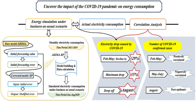
The existing measurement of the impact of the COVID-19 pandemic on energy consumption is based on changes between the years, which demonstrates the changes in energy consumption over the years without fully reflecting the impact of the pandemic on energy consumption. To better uncover the impact of the COVID-19 pandemic on energy consumption, this research compared pandemic-free scenarios with actual (with COVID-19) energy consumption in 2020, rather than comparing energy consumption between 2020 and 2019 in the existing studies. The simulation approach used for scenario simulation was developed by combing the autoregressive integrated moving average (ARIMA) and back propagation neural network (BP). In the proposed ARIMAR-BP approach, BP was used to correct the error of ARMIA simulation, so as to reduce the error of simulation. The results of the model testing indicate that the simulation error of the developed approach is much lower than that of the BP or ARIMA simulation. The proposed simulation approach was run based on China's electricity consumption from 2015 to 2019 to produce the simulated value of China's electricity consumption from January to August of 2020 in the pandemic-free scenario. The actual electricity consumption was on average 29% lower than the electricity consumption in the pandemic-free scenario. which is much larger than the decline rate derived from year-to-year comparison. In addition, the results of the correlation analysis show the simulated decline in electricity consumption is only positively correlated with the number of new cases of COVID-19 in January–March, when the COVID-19 outbreak in China. This research provides a novel research structure for a more comprehensive understanding of the impact of the pandemic on energy consumption.
Keywords: COVID-19, Power consumption, Business-as-usual scenario, Simulation
Graphical abstract
1. Introduction
The lockdown measures to contain the outbreak of the COVID-19 pandemic lead to a decline in energy consumption. According to the Monthly Electricity Statistics released by International Energy Agency, global electricity consumption fell by 8.6% in 2020 compared with 2019. That compares with 6.6% in the United States and 0.8% in China (IEA, 2020). Such measurement reflects the year-to-year changes in energy consumption, which fails to fully reflect the impact of the pandemic on energy consumption. To fill the research gap as well as to better assess the true impact of the pandemic, this work developed a new research framework to compare the energy consumption in the business as usual (without COVID-19 pandemic) scenario with in the actual outbreak of COVID-19 in 2020. The difference between the business as usual scenarios with actual energy consumption was regarded as the decrease in energy consumption caused by COVID-19. Research has provided a new way to assess the impact of COVID-19 on energy consumption and was of vital help in meeting the energy challenges caused by the COVID-19 pandemic.
An empirical analysis of China's electricity consumption using the proposed research framework was conducted. Specifically, the ARIMA-BP model with improved strategy was used to simulate the virtual electricity consumption under the business-as-usual scenario. After that, the business-as-usual scenario electricity consumption was compared with the actual electricity consumption. The difference was assumed to be the decline in electricity consumption caused by the COVID-19. For further analysis, this study conducted the correlation between the electricity declines and the number of confirmed cases. Analysis conclusion can not only be conducive to a comprehensive understanding of China's energy shocks caused by the COVID-19, but also reveal how China's recovery has fared over different periods of the pandemic.
The structure of this article is as follows: The second section is literature reviews. The third section is the methodology, including data sources, framework diagrams and model formulas. The fourth section is result analysis, including the electricity consumption decline calculation and correlation analysis. The fifth section summarizes the whole paper.
2. Literature reviews
2.1. Literature review on the impact of extreme on energy
As a sudden pandemic, COVID-19 exerted varying degrees of impact on all walks of life in the whole society (Wang and Su, 2020). From the past to the present, the hot spots after historical emergencies have reference significance for today's events. Analyzing from past research, assessing the impact of the event has become the primary concern of scholars and the community. Taking the 2008 financial crisis event as an example, this sub-section focused on sorting out the research connected with this event, in order to obtain research ideas.
Many scholars have sorted out the impact of the 2008 financial crisis on all aspects of society, covering financial markets, technological innovation, oil prices, and energy consumption (Jin, 2016). The first is the financial market. Scholars have drawn a series of conclusions by analyzing and comparing the volume of the financial market before and after the crisis. Hasan and Mohammad (2015) used MF-DFA technology to study the multifractal structure of the US and seven Asian stock markets during the financial crisis. The study found that the markets of the United States, Japan, Hong Kong, South Korea, and Indonesia exhibit strong non-linear relationships. Based on the monetary and fiscal performance of the global financial crisis in 2008–09, Makin (2019) reviewed the performance of Australia's global financial crisis and emphasized the effectiveness of the macroeconomic actions at that time. Outside the economic field, Brem et al. (2020) assessed the impact of the financial crisis on innovative industries. Based on vertical patent data from the OECD, the study found the negative impact of the global financial crisis on innovation performance. Focusing on the field of crude oil, Lahmiri (2017) investigated the state and performance of oil prices before and after the international financial crisis. It has been shown that after the international financial crisis, the volatility of Brent and West Texas Intermediate (WTI) both showed chaotic dynamics. Also investigating the crude oil market are Joo et al. (2020). In their study, Hurst index, Shannon entropy and scaling index are used to characterize the efficiency and long-term equilibrium changes of the oil market caused by the financial crisis. Moutinho et al. (2017) compared and analyzed the relationship between crude oil prices in the European Union and consumer prices of transportation fuels before and after the 2008 financial crisis. Studies have found that there is a close correlation between crude oil and gasoline prices, but there does not seem to be a similar relationship in the post-breakthrough period. In the energy field, scholars compared the data in the late period of the crisis with the data in the current period of the crisis, and obtained the amount of influence based on the input-output method. With the aid of data that has occurred in 2008 and 2009, Yuan et al. (2010) discussed the impact of the 2008 financial crisis on China's energy consumption and economic growth. Through the calculation of the input-output model, they found the percentage of the impact of the crisis in 2008 and the economic stimulus in 2009 on the economy and the energy industry respectively. Similar to the Chinese case, Ali Bekhet and Yasmin (Ali Bekhet and Yasmin, 2014) studied the impact of the financial crisis case on Malaysia. It turned out that the financial crisis has led to a 13% drop in GDP and a 16% drop in energy consumption.
Through the above analysis, we found that studying the impact of emergencies on various sectors of society has become a practice of taking history as a mirror. However, most of the previous studies primarily analyzed the performance of multiple industries after the incident through inter-year comparisons. This measurement had a certain degree of lag and could not make timely judgments from the perspective of the impact of the event itself. To avoid this situation, a timely judgment of the event's impact from the perspective of scenario simulation in time is a feasible way. To do this, appropriate energy simulation methods can provide a solution.
2.2. Literature review on scenario simulation methods
Data fitting under simulated scenarios can quantify the specific impact of the pandemic on energy consumption. Specifically, we expected to adopt mature methods to achieve accurate simulation of electricity consumption in the absence of an pandemic. To realize this idea, this sub-section combed and summarized the research progress related to energy simulation. The combing of the literature was of vital help to refine research methods and simulation calculations.
In the field of energy fitting and simulation, method research around time series data was an important point. Many scholars have carried out related researches around ARIMA model and GM model. Selvaraj et al. (2020) affirmed the importance of statistical analysis of the ARIMA model. The ARIMA model has recently been widely used in the simulation of pandemics (Duan and Zhang, 2020). Hernandez-Matamoros et al. (2020) used the ARIMA model to simulate the spread of the COVID-19 virus in 15 countries around the world. Singh et al. (2020) used wavelet and ARIMA coupling to develop a new hybrid model to simulate the number of deaths caused by COVID-19 in major countries around the world. Simulations show that despite the various preventive measures taken by the governments of these countries, the number of deaths will continue to increase sharply. Khan and Gupta (2020) used a univariate time series model to simulate the number of COVID-19 cases in India that might be infected in the next 50 days. Jamil (2020) modeled ARIMA to simulate water consumption in Pakistan. Wang et al. (2018b) used a new hybrid of nonlinear gray model and linear ARIMA residual correction to simulate U.S. shale oil production in order to better understand the global oil market. Al-Musaylh et al. (2018) forecasted the short-term electricity demand of Queensland, Australia's second largest state, based on the ARIMA model. Through bagging ARIMA and exponential smoothing method, de Oliveira and Cyrino Oliveira (2018) simulated the medium and long-term power consumption of different countries/regions. Use autoregressive integrated moving average (ARIMA) and seasonal ARIMA (SARIMA) methods, Ediger and Akar (2007) estimated Turkey's future primary energy demand from 2005 to 2020. In addition to the above studies, there are also too many studies that combine the ARIMA model with other models for simulating (Koutroumanidis et al., 2009) (Barak and Sadegh, 2016). Ji et al. (2019) uses the ARIMA model and a deep neural network structure combining CNN and LSTM layers to simulate the price of carbon futures (Bowden and Payne, 2008).
Apart from time series models, the research work of artificial neural networks was also deepening, and great progress had been made. There were numerous researches on this subject by related scholars. Di Piazza et al. (Di Piazza et al., 2020) studied an artificial neural network (ANN)-based model for short-term simulating of hourly wind speed, solar radiation, and electricity demand. The simulation analysis proved that the method could coordinate the good prediction performance in the short term with a very simple network structure. Rodríguez et al. (2018) proposed an artificial neural network (ANN) to simulate photovoltaic generators. Dumitru and Gligor (2017) established an architecture based on a feedforward artificial neural network and simulated the daily average wind energy in Southeast Europe. Using Iran's monthly available data from 1996 to 2006, Azadeh et al. (2013) used an artificial neural network (ANN) method to simulate the consumption of renewable energy in consideration of environmental and economic factors. Neto and Fiorelli (2008). Pino et al. (2008) used an artificial neural network to simulate the next day's electricity price in the Spanish energy market. Moreira et al. (2021) used an artificial neural network (ANN) to estimate the photovoltaic power generation in Minas Gerais, Brazil, with an average absolute percentage error of 4.7% per week. Khwaja et al. (2020) used integrated machine learning based on artificial neural networks (ANN) to perform short-term power load forecasting in New England. Islam et al. (1995) developed a new type of artificial neural network (ANN) to simulate electricity load and energy in the next 24 months. The artificial neural network model has also been applied to the simulate of European electricity load (Behm et al., 2020) and wind power generation (Zafirakis et al., 2019). In addition, combination models related to artificial neural networks are also common in practical applications (Zainuddin et al., 2019).
Through the above combing, it can be found that the existing fitting methods are relatively mature and have good practice for solving energy simulations in different situations. On the one hand, the ARIMA model and BP model have higher practicability and accuracy in methods of energy simulating. Energy simulation based on these two types of models is generally applicable to electricity, oil and gas, etc. On the other hand, the combination of multiple methods has become popular in the latest research. If we want to achieve further improve in accuracy, the construction of a compound model based on a new combination of ideas is necessary. This part of the combing provides the idea that, it is feasible to apply these two methods to determine the amount of electricity consumption in a pandemic-free state. In this way, the quantitative treatment of the impact on the pandemic could be realized.
2.3. Contribution points of this research
Through combing the existing research, we found that the current study of extreme events' impact on energy consumption was based on changes between years, which showed the inter-annual relative changes in energy consumption but did not fully reflect the immediate impact of emergency events on energy. In order to consider the specific effect from the incident itself, simulating the assumed amount of energy in the absence of a pandemic was the solution. Energy simulation methods have a certain degree of research enthusiasm in the current research field. Simulation methods that focus on combined models are the most common and accurate. By combing of these two points, this research aimed to design a research framework that used new energy simulation methods to assess the specific impact of China's electricity consumption caused by the pandemic.
In summary, the contributions of this research mainly included the following points. (1) First of all, this research designed a research framework to compare the electricity consumption of the whole Chinese society under the business-as-usual scenario and the actual scenario. The difference between the two was regarded as the loss value of the electricity industry affected by the pandemic. (2) Secondly, this research further optimized the existing mature energy simulation methods. A combination mechanism of "error correction + secondary modeling" has been established. Relying on this mechanism, a combined "ARIMA-BP" model was created. The comparison between multiple models helps to ensure whether the simulation mechanism in the combined model is superior, thereby providing persuasive results for the research. (3) The study further analyzed the correlation between the decline in the electricity industry and the severity of the pandemic. This relevant analysis played an important role in explaining the epidemic-driven reasons behind the downward trend. In general, this research has adopted mature methods to simulate the impact of the pandemic on China's electricity consumption. It could provide a reference value for the relevant research between the pandemic and China's energy, economy, and industries in the current context.
3. Method
3.1. Framework of this study
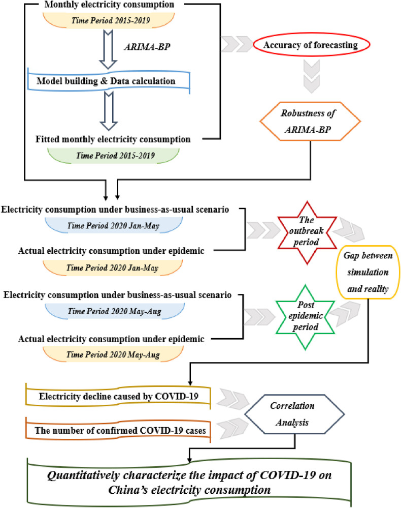
This work designed a research framework to quantitatively analyze the difference between the business-as-usual scenario and the actual scenario in 2020. Specifically, by modeling the monthly electricity consumption data from 2015 to 2019, China's electricity consumption in 2020 derived from the historical trajectory was simulated. There were two reasons for choosing electricity consumption as the research object. First, electricity consumption accounts for most of a country's energy use. Evaluating the impact of the epidemic on electricity consumption can reflect changes in the energy sector under the epidemic. Secondly, electricity consumption is related to all aspects of the operation of a country's society, so it is the best indicator to evaluate the extent to which a country's society is affected/recovered by the epidemic. Overall, the electricity consumption used in this research can not only reflect the comprehensive state of the energy field, but also reflect the social conditions beyond the energy field. Therefore, electricity consumption is an ideal social assessment indicator under the epidemic environment. Among multiple simulated methods, the autoregressive integrated moving average model (ARIMA model) and backpropagation neural network model (BP model) are used as traditional models. In addition, the ARIMA-BP model newly constructed in this research based on the principle of “error correction and secondary modeling” was applied to the simulation of this research. Mean square error (MSE), mean absolute percentage error (MAPE) and mean square error percentage (MSPE) was used to calculate the accuracy of these methods. The simultaneous use of multiple methods increased the persuasiveness of the simulation results. After that, we compared the electricity consumption in this ideal state with the actual monthly electricity consumption in 2020.
This gap in electricity consumption was regarded as the absolute amount of the decline in electricity consumption caused by the pandemic. Furthermore, analyzing the correlation between this decline and the severity of the pandemic could assess the stagnation and recovery state of Chinese society during the pandemic. Based on this research framework (as shown in Fig. 1 ), this study provided a new way to quantitatively measure the impact of the pandemic. The results of the study were of vital help for the macro-understanding of the supply and demand security of the energy market under the pandemic.
Fig. 1.
The framework of this study.
3.2. Data description
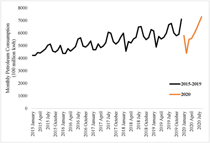
The data used in this paper come from China Electricity Council (2020). With the pandemic from severe to mild, China has gradually shifted from industry closure to industry recovery, and the process of social restart has also begun. Thus, electricity consumption in 2020 is significantly different from previous years. Fig. 2 shows China's electricity consumption over the period 2015–2020. The black line in the figure represents the historical value from 2015 to 2019, and the yellow line represented the value in 2020. The black curve displays that China's petroleum consumption presents an overall upward trend with seasonal characteristics in history. The electricity consumption in 2020 shown by the Yellow curve indicates a trend of decreasing first and then rebounding quickly. These data characteristics, which are different from those in previous years, further confirm the obvious impact of the pandemic on China's electricity consumption.
Fig. 2.
Monthly petroleum consumption in China period 2015–2019.
3.3. Simulating technique
Existing models establish accurate equations based on the characteristics of historical data when simulating, so as to obtain prediction results that conform to the law of historical fluctuations. With the development of simulating technology, different models have their own advantages in establishing electricity consumption simulations. Therefore, the comparison and combination of models has become the key to improving the accuracy of prediction. In order to make the prediction more accurate, we use combination method based on error correction principle to simulate the electricity consumption in 2020. The rest of this section focused on these methods.
3.3.1. ARIMA model
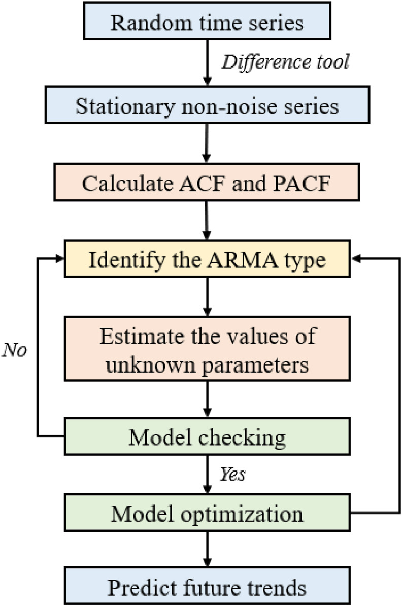
The Autoregressive Integrated Moving Average Model (ARIMA) is a method of establishing a mathematical model through curve fitting and parameter estimation (Zhang, 2003). This model is mainly for stationary non-white noise sequence data, and generally uses a specific mathematical formula to make the data meet the calculation conditions (Morimune and Miyazaki, 1997). In the process of transforming a non-stationary time series into a stationary time series, the ARIMA model is a model established by regressing the dependent variable only on its lag value and the present value and lag value of the random error term. This reflects that the ARIMA model has the characteristics of simple operation. Its modeling only needs endogenous variables and does not need to resort to other exogenous variables. At the same time, the ARIMA model also has its application limitations. First of all, the model has strict requirements on the stability of the data. Stationarity can be divided into two categories: strong stability and weak stability. In the process of practical application, strong stationarity is too ideal and theoretical, and weak stationarity and unevenness need to be dealt with by difference tools. If the data after the difference is still not stable, then this set of data series could not be executed. Secondly, the ARIMA model essentially can only capture linear relationships, not non-linear relationships. The overall flow chart is shown in Fig. 3 .
Fig. 3.
Flow chart of ARIMA model.
In the first step of model calculation, the elimination of random factors in the time series is the first consideration. Differential tools are usually applied to this process (Hillmer and Tiao, 1982). The D-order difference tool can make the original series {} into a stationary series {}. The specific steps are as follows:
| (1) |
After the conversion of stationary non-white noise data, the autocorrelation function (ACF) and partial autocorrelation function (PACF) of the model are calculated in the second step.
The determination of autocorrelation and partial autocorrelation coefficients can identify the type of the model on the one hand and determine the parameters on the other hand. The autocorrelation function of AR (p) model is expressed as:
| (2) |
MA (q) is the use of current error terms and the previous period of error items to explain the explanatory variables. The partial autocorrelation function of MA (q) model is expressed as:
| (3) |
Where c means constant variable; means parameter; means error terms.
If a model has both the above nature of the AR (p) and MA (q) process, then it can form an autoregressive and moving average process ARMA (p, q) model:
| (4) |
Finally, after model testing and optimization, the future trend of the data can be predicted.
3.3.2. BP model
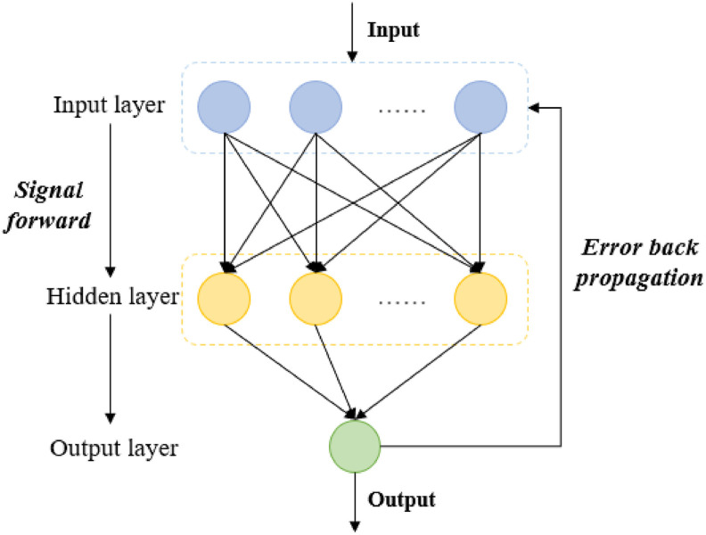
BP neural network model was a commonly used neural network learning algorithm. This model was applied in the field of energy simulation in the 1990s (Hobbs et al., 1998) and has been used more and more widely recently (Hsu et al., 2018). The calculation process includes two steps of signal forward propagation and error backward propagation. Among them, the forward propagation of the signal refers to the data from the input layer through the hidden layer to the output layer. Backward propagation of errors refers to error analysis based on the training results and expected results, and then modify the weights and thresholds, step by step to obtain a model that can output consistent with the expected results (Li and Wang, 2019). The specific principles of the training process of the BP neural network model are as follows (as shown in Fig. 4 ):
Fig. 4.
Flow chart of BP neural network model.
The beginning of model training is to establish the transfer function (Sigmoid function) between the input layer and the hidden layer:
| (5) |
While the function between hidden layer and output layer is Purelin function.
The second is to determine the number of nodes in the hidden layer and the output layer. Among them, the function for determining the number of nodes in the hidden layer is: , where K means sample number; means the number of hidden layer's node; n means the number of input layer's node; and = 0 if i > n (He et al., 2007).
After the forward propagation process, the next step is to reverse the error. In this process, errors are propagated from the output layer back to the hidden layer, and then back to the input layer. Through the layer-by-layer correction of the weight matrix, the goal of optimal output is achieved. The errors are calculated by formula (6) where represents error, means the expected output and means actual output.
| (6) |
| (7) |
| (8) |
The adjustment formulas of the weight matrix and the threshold matrix are shown in equations (9), (10). The partial derivative of the weight coefficient error is the key to finding the optimal result. After the above series of calculations, the actual output can be consistent with the expected output. The prediction results based on this process are quite convincing.
| (9) |
| (10) |
3.4. Error correction mechanism and ARIMA-BP model
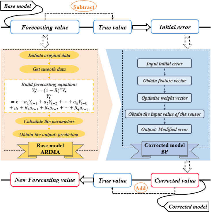
Based on the existing ARIMA model and neural network model, this research put forward the modeling principle of "error correction" combined with the idea of further improving the prediction accuracy. This idea combined the above two models by selecting the base model and the modified model. The accuracy was improved through the secondary correction of the error.
During error correction modeling principle, it first extract the prediction error based on the base model; then use the correction model to perform residual correction, that is, perform a secondary prediction on the error given by the initial model to achieve the effect of reducing the error. By combining the results of the initial model with the errors of the modified model, the optimal prediction value has been obtained. The detailed modeling principle is shown in Fig. 5 .
Fig. 5.
The detailed error correction modeling principle.
Combining this principle, ARIMA-BP combined model was applied in this study. The ARIMA-BP model was a combination based on the principle of "error correction + secondary modeling". Among them, the ARIMA model was the first step in operation, and the initial error is the product of this step. After this, the initial error was substituted into the calculation of the BP software. Through the secondary modeling, the corrected error and the final prediction result of the ARIMA-BP model were obtained (Wang et al., 2018a). The operating formula and steps of the ARIMA-BP model were shown below.
-
(1)
Use tools such as unit root test and difference to make the initial data series stable. Among them, the formula of unit root test is: . This is to judge the stability of the data. The formula of the difference tool is: . In this step, the non-stationary series is treated as a stationary series through a formula.
-
(2)
We bring the data that has become stable after processing into the ARIMA model to solve the preliminary prediction results. Model identification, model ordering, and parameter estimation need to be processed sequentially in the whole process. Model recognition is to judge the type of model. AR model is: . MA model is: . Model order is determined by the BIC criterion method. Parameter estimation is to solve the two unknown parameters “p” and “q” in the equation.
-
(3)
Run the ARIMA model to get the initial prediction results. By subtracting the predicted value of this step from the true value, the initial prediction error is obtained.
-
(4)
Input the initial error into the BP model (Dumitru and Gligor, 2017) to generate the BP network. Then conduct network training and simulation. Among them, the formula for network training is as follows: . The formula for network simulation is as follows: . Through the operation of the software, the corrected error sequence is calculated.
-
(5)
Combine the corrected error sequence with the initial prediction value to get the final prediction result.
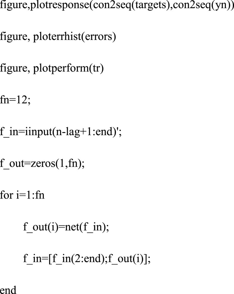
The tools used to run the model are Eviews, SPSS and Matlab software. Among them, Eviews is used to process the stability of the data and to determine the parameters of the ARIMA model, and the SPSS software is used to run the initial prediction results of the ARIMA model. Matlab software is used to simulate the BP program of the initial error, and the error after the second correction is obtained. The prediction result of this research was obtained after integrating the three software operations. Among them, Eviews and SPSS are operations within the software, while Matlab relies on data codes. The data code was shown in the appendix.
4. Empirical result and analysis
4.1. Hypothesis of electricity consumption without an pandemic
To model the monthly electricity consumption from 2015 to 2019, this sub-section mainly focused on the prediction process and accuracy of each model. According to statistics from the China Electricity Council, the value of electricity consumption in the past five years was shown in Table 1 . The data conveyed the following information points. First, China's electricity consumption had shown a slow upward trend in the past five years. Specifically, the annual growth rate in recent years was 18%, 22%, 21%, 5%, and 15%. Second, there were apparent seasonal changes between monthly data. Summer and winter usually reached small peaks of electricity consumption during the year.
Table 1.
Historical monthly electricity consumption data in China (100million kwh).
| Month | Year |
||||
|---|---|---|---|---|---|
| 2015 | 2016 | 2017 | 2018 | 2019 | |
| January | 4227 | 4381 | 4678 | 5995 | 6172 |
| February | 4227 | 4381 | 4678 | 4557 | 4891 |
| March | 4448 | 4762 | 5139 | 5325 | 5732 |
| April | 4415 | 4569 | 4847 | 5217 | 5534 |
| May | 4567 | 4730 | 4968 | 5534 | 5665 |
| June | 4723 | 4925 | 5244 | 5663 | 5987 |
| July | 5034 | 5523 | 6072 | 6484 | 6672 |
| August | 5124 | 5631 | 5991 | 6521 | 6770 |
| September | 4563 | 4965 | 5317 | 5742 | 6020 |
| October | 4491 | 4890 | 5130 | 5481 | 5790 |
| November | 4658 | 5072 | 5310 | 5647 | 5912 |
| December | 5023 | 5369 | 5703 | 6283 | 7110 |
By fitting the data, the historical values derived from the simulated model were calculated. This sub-section showed the deduction process of each model in turn. Indicators for judging the accuracy of model fitting was given.
4.1.1. Model fitting of BP
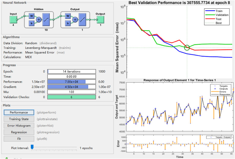
According to the calculation steps listed in the previous section 3.3, this study uses Matlab software to perform a fitting operation on electricity consumption by BP model.
Fig. 6 was a diagram of the internal calculation process of the BP model. It can reflect the continuous correction and test process of the error in the inner calculation. Through the reverse adjustment process of the error, the best validation performance was 307555 at epoch 8. In addition, the error curve obtained after optimization was also included in the plan. After the positive and negative feedback mechanism inside the model, the fitting results were shown in Table 2 . It was worth noting that model's accuracy could be calculated by comparing the data in Table 1, Table 2. This detailed part was placed in Section 4.1.3.
Fig. 6.
The flow chart of internal operation of BP model.
Table 2.
Initial fitted result based on the BP model.
| Month | Year |
||||
|---|---|---|---|---|---|
| 2015 | 2016 | 2017 | 2018 | 2019 | |
| January | 4227 | 5054 | 5456 | 5888 | 5967 |
| February | 4227 | 4549 | 4549 | 5588 | 5751 |
| March | 4448 | 4849 | 4991 | 5128 | 5581 |
| April | 4415 | 5055 | 5054 | 5555 | 6695 |
| May | 4535 | 4549 | 4549 | 5283 | 4968 |
| June | 4677 | 4828 | 5008 | 5709 | 5575 |
| July | 4777 | 5040 | 5054 | 5134 | 6116 |
| August | 5052 | 5629 | 5942 | 6364 | 6773 |
| September | 4959 | 5089 | 5551 | 5756 | 5992 |
| October | 4549 | 4952 | 5129 | 5582 | 6067 |
| November | 4923 | 5265 | 5575 | 5980 | 6299 |
| December | 5298 | 5313 | 5761 | 6004 | 6818 |
4.1.2. Model fitting of ARIMA-BP
The first step of the ARIMA-BP model is to use the ARIMA model to make initial predictions. After this, the initial prediction error was obtained by calculating the difference between the two. Then, we used the correction function of the BP model to correct the initial error.
The ARIMA model first performed a unit root test on the data. Since the data had specific fluctuation characteristics, this process was essential and could not be omitted. Table 3 was the result of the unit root test. Among them, Q represents the original sequence, Q* means the sequence after the first-order difference, and Q** represents the sequence after the second-order difference. By comparing the ADF statistic with the value of different confidence intervals (1%, 5%, and 10%), the stable characteristics of the data were reflected.
Table 3.
Unit root test and difference results based on Eviews 7.2
| Sequence | ADF Statistic | Critical Value |
Value of p | ||
|---|---|---|---|---|---|
| 1% | 5% | 10% | |||
| Q | −7.894837 | −4.156734 | −3.504330 | −3.181826 | 0.0000 |
| Q* | −13.37168 | −4.161144 | −3.506374 | −3.183002 | 0.0000 |
| Q** | −7.008416 | −4.165756 | −3.508508 | −3.184230 | 0.0000 |
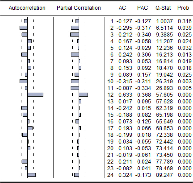
Through continuous inspection, the fitting accuracy of the data was the most accurate in the first-order difference. Based on this, the correlation coefficient map of the first-order difference sequence was drawn and the values of “p” and “q” in the ARIMA model were determined. The autocorrelation coefficient graph and partial autocorrelation coefficient graph in Fig. 7 were obtained through Eviews7.2 software. By judging their respective convergence conditions, it can be roughly determined that the partial autocorrelation coefficient was truncated after the third order. The autocorrelation coefficient was truncated after the second order. In addition, the values of Prob were all less than 0.05 which meaned that the selection of parameters has a higher reliability. In summary, ARIMA (3, 1, 2) was chosen.
Fig. 7.
Autocorrelation and partial autocorrelation coefficients of the original sequence.
In order to further confirm this point of view, we calculated the stationarity R-square of the ARIMA model fitting. The results confirmed that the selection of parameters was reliable. Table 4 further listed the fit significance and the number of outliers, confirming the validity of the prediction.
Table 4.
Parameters of fitting goodness for ARIMA (3,1,2) model.
| Model | Number of Predictors | Model Fit Statistics |
Number of Outliers | |
|---|---|---|---|---|
| R-Squared | Significance | |||
| ARIMA (3,1,2) | 1 | 0.630 | 0.000 | 0 |
After the above calculations, the initial prediction values of the final ARIMA (3, 1, 2) model were shown in Table 5 . By comparing the difference between the results in Table 5, Table 1, the initial errors were listed as input of BP model. Through the calculation of the BP model, the running results of the ARIMA-BP model were obtained (see Table 6).
Table 5.
Initial fitted result based on the ARIMA model.
| Month | Year |
||||
|---|---|---|---|---|---|
| 2015 | 2016 | 2017 | 2018 | 2019 | |
| January | 4227 | 4381 | 4678 | 5995 | 6172 |
| February | 4227 | 4381 | 4678 | 4557 | 4891 |
| March | 4448 | 4762 | 5139 | 5325 | 5732 |
| April | 4415 | 4569 | 4847 | 5217 | 5534 |
| May | 4567 | 4730 | 4968 | 5534 | 5665 |
| June | 4723 | 4925 | 5244 | 5663 | 5987 |
| July | 5034 | 5523 | 6072 | 6484 | 6672 |
| August | 5124 | 5631 | 5991 | 6521 | 6770 |
| September | 4563 | 4965 | 5317 | 5742 | 6020 |
| October | 4491 | 4890 | 5130 | 5481 | 5790 |
| November | 4658 | 5072 | 5310 | 5647 | 5912 |
| December | 5023 | 5369 | 5703 | 6283 | 7110 |
Table 6.
Finial predicted result based on the ARIMA-BP model.
| Month | Year |
||||
|---|---|---|---|---|---|
| 2015 | 2016 | 2017 | 2018 | 2019 | |
| January | 4227 | 4589 | 5033 | 6095 | 6223 |
| February | 4228 | 4927 | 5246 | 4604 | 5544 |
| March | 4230 | 4782 | 5118 | 5015 | 5387 |
| April | 4413 | 4199 | 4621 | 6017 | 6130 |
| May | 4994 | 5114 | 5108 | 5707 | 6051 |
| June | 4777 | 4851 | 5217 | 5620 | 5821 |
| July | 4811 | 5275 | 5789 | 5933 | 6342 |
| August | 5109 | 5430 | 5436 | 6007 | 6385 |
| September | 4555 | 5071 | 5554 | 5917 | 6410 |
| October | 4820 | 5003 | 5182 | 5361 | 6094 |
| November | 4690 | 4949 | 5172 | 5752 | 6185 |
| December | 4561 | 4878 | 5412 | 5843 | 6696 |
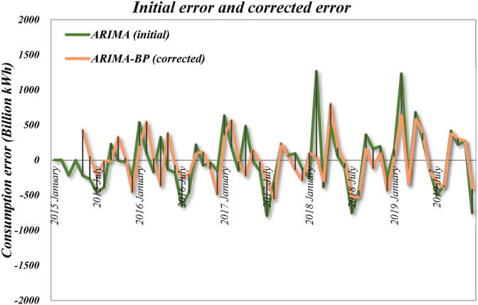
The calculation of the BP model was similar to the previous one. After positive propagation and negative feedback, the corrected error sequence was shown in Fig. 8 (orange lines). It can be seen from the figure that the orange curve was closer to the coordinate axis than the green curve.
Fig. 8.
Comparison chart of initial (ARIMA) and corrected error (ARIMA-BP).
4.1.3. Accuracy comparison analysis
In this study, we compared the accuracy of the different models using the fitted data and used the comparison between the real value and the simulated value to calculate the error value. The more common error value formula has the following. In these error formulas, we define ‘’ ‘’ ‘’ as fitting value, true value and sample size, respectively. Detailed error judgment indicators were mean absolute percent error (MAPE), mean square percent error (MSPE) and mean square error (MSE).
The MAPE (Mean Absolute Percent Error) was used to measure the accuracy of prediction, and calculation formula was:
| (16) |
Where: is predicted value, is actual value, n is the number of data.
The smaller the average relative error is, the higher the prediction accuracy is.
In these expressions, is the predicted value and is the actual value.
The mean square error (MSE) was calculated as follows:
| (17) |
Where: is predicted value, is actual value.
The mean square percent error (MSPE) was calculated as follows:
| (18) |
By comparing the predicted value and actual value, the prediction error of each model was calculated in Table 7 . For the MAPE value, the value of the combined ARIMA-BP model was smaller than that of the ARIMA and BP models. In addition, the MSPE and MSE values of the combined model were also smaller than those of the two single models. This proved that the predictive effect of the integrated model was more accurate than the two single models. Therefore, the prediction results based on the combined model were more convincing.
Table 7.
MAPE, MSPE and MSE calculated for each model (%).
| Type | BP | ARIMA | ARIMA-BP |
|---|---|---|---|
| MAPE | 5.25% | 6.05% | 4.98% |
| MSPE | 0.009986653 | 0.010021953 | 0.007750388 |
| MSE | 171545.1371 | 165270.6099 | 101911.7331 |
4.2. Electricity consumption gap caused by the COVID-19
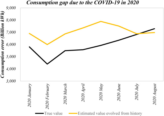
By comparing the prediction results of the ARIMA-BP model with the actual statistics, the electricity consumption gap caused by the 2020 pandemic could be calculated. Table 8 listed this point numerically, while Fig. 9 ploted the gap curve between the two from an image perspective.
Table 8.
The difference in China's electricity consumption in 2020 with or without the pandemic (100million kwh).
| Month | Simulations of ARIMA-BP | Real value of 2020 | Consumption gap | Decline proportion (%) |
|---|---|---|---|---|
| January | 6906 | 5805 | 1101 | 18.96% |
| February | 5997 | 4398 | 1599 | 36.36% |
| March | 6870 | 5493 | 1377 | 25.06% |
| April | 7359 | 5572 | 1787 | 32.08% |
| May | 7893 | 5926 | 1967 | 33.19% |
| June | 7515 | 6350 | 1165 | 18.34% |
| July | 6885 | 6824 | 61 | 0.90% |
| August | 6979 | 7294 | −315 | −4.33% |
Fig. 9.
Electricity consumption gap caused by COVID-19.
According to the data in Table 8, compared with the historical expected trajectory, the decline in electricity consumption from February to May was the largest, ranging from 25% to 36%, with an average of 30%. Since June, the gap between the actual value of electricity consumption and the ideal value has gradually narrowed. This rate of decline fell from 18% in June to 0.9% in July. At this point, the positive gap began to stop. With the advent of the post-pandemic era, the actual electricity consumption finally exceeded the expected electricity consumption for the first time in August, and the exceeding rate remained at 4.33%.
The yellow curve in Fig. 9 was the ideal value of electricity consumption in China without the pandemic generated by the ARIMA-BP model in this study. The black curve was the actual value of electricity consumption in 2020. These two curves showed irregularly shaped gaps during the period from January to July. Since July, the gap between the two lines began to become smaller. After that, the actual electricity consumption began to exceed the expected value, and there was a characteristic that the excess volume became larger and larger.
In this study, we regarded the area enclosed by the two curves in Fig. 9 as a quantitative value of the impact of the pandemic on China's electricity consumption. The gap between the two curves was closely related to the severity of the pandemic to a certain extent.
Since the outbreak of COVID-19, the pandemic in China has experienced an incubation period, a severe period, and a post-pandemic period. In terms of specific months, from February to March, the number of new cases has always remained high. The tense atmosphere of the masses forced the slowdown of society and hindered travel. By April–May, although the number of new cases was under control, people were still very concerned about maintaining social distancing. The social part was functioning normally, but the operations of many offline entities were still prohibited due to people's panic. Since entering June, this panic has gradually subsided. To restore the economy, the social resumption of work and production has started to accelerate the process. At the same time, domestic inter-provincial transportation and entertainment activities have also begun to expand.
From this analysis, industrial and commercial activities in society have shown a dynamic change during the pandemic. Consistent with this change, the decline in electricity consumption in China's entire society during the pandemic was also following this process and undergoing fundamental changes. Based on this essential judgment, this study believed that it was necessary to give a detailed statistical analysis of the correlation between the two. This kind of correlation analysis can assist in understanding the reasons behind the change in the electricity consumption gap. In the long run, this analysis also provided a reference for predicting the supply and demand trends of the energy market in future emergencies.
4.3. Correlation analysis between gaps and confirmed COVID-19 cases
This sub-section calculated and analyzed the correlation coefficient between the electricity consumption gap and the pandemic (see Table 9 ). It was expected to obtain the variation curve of the specific value of the correlation coefficient.
Table 9.
Correlation test results between gaps and confirmed COVID-19 cases.
| Period | Variable | Correlation test | Result |
|---|---|---|---|
| January to March | Gaps | Pearson correlation coefficient | 1.000** |
| Significance (two-tailed) | 0.000 | ||
| Number of cases | 3 | ||
| March to May | Cases | Pearson correlation coefficient | −1.000** |
| Significance (two-tailed) | 0.000 | ||
| Number of cases | 3 | ||
| May to August | Cases | Pearson correlation coefficient | −1.000** |
| Significance (two-tailed) | 0.000 | ||
| Number of cases | 4 |
Note: ** means the correlation is significant at the 0.01 level (two-tailed).
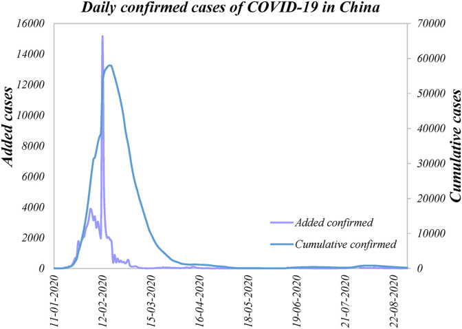
Fig. 10 showed the changes in the cumulative number of confirmed cases and the number of newly confirmed cases in China recorded from the official website of the China Health Commission. Among them, the purple curve showed the data of newly confirmed cases each day, and the blue curve displayed the cumulative number of confirmed cases that day. Although the meanings of the two curves were different, they showed a consistent range of change. Monthly, the number of cases began to appear in January and reached a climax in February at a rapid rate. In mid-to-late February, the cumulative number of confirmed cases in China reached a peak of 58,000. The number of new cases also achieved the highest during that period, with 15,000 cases. Since this peak, the cumulative number of confirmed cases in China has gradually declined since March. After a two-month decay period, the cumulative number of confirmed cases in China fell to a stable minimum at the end of April. We also call the period during which the total number of cases remained within 300 cases as the post-pandemic period.
Fig. 10.
Daily confirmed cases of COVID-19 in China.
Return to the research object of this study. According to existing analysis, electricity consumption is directly determined by social and industrial conditions. Since 2020, social and industrial conditions have been largely affected by the pandemic. From this reasoning, the dynamic evolution of the entire pandemic should theoretically be related to the gap in electricity consumption.
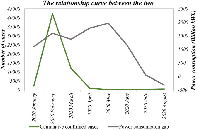
To verify the relationship between the two, this section first draws the curves of gaps and cumulative confirmed cases. As shown in Fig. 11 , the green curve represents the cumulative number of confirmed cases, and the dark gray curve represents the calculated gap in electricity consumption. It can be seen from the figure that there are different correlations between the two in different periods of change. From January to March, the cumulative number of confirmed cases showed rising first and then falling. At the same time, the electricity consumption gap showed the same characteristics of rising first and then falling. Judging from the reasons behind it, these few months correspond to the most severe period of the pandemic in China. The positive correlation between the two was related to restrictive measures. Specifically, the severity of the pandemic has strengthened the implementation of restrictive measures such as suspension of work and production. The rest of work and production and transportation restrictions have increased the impact of the pandemic on the electricity industry, resulting in a growing gap between the expected value of electricity consumption and the actual value. From this perspective, there is a clear positive correlation between the pandemic and the gap in January–March.
Fig. 11.
Relationship curve between electricity gaps and confirmed COVID-19 cases.
In March–May, the cumulative number of confirmed cases dropped and returned to a stable level, and the pandemic situation showed a significant improvement. At the same time, the gap has not gradually become smaller, but still showed upward characteristics. This meaned that during this period, although the pandemic was under control, the electricity consumption of the whole society has not returned to the ideal scenario (the same as in previous years). The reason for this phenomenon was closely related to people's psychological panic about the pandemic. Due to prolonged immersion in the anxiety brought about by the pandemic, the industrial production, commercial scale, and transportation of the whole society have still not recovered to the level when it was completely unaffected. Therefore, during this period of time, the electricity consumption gap did not decrease as the number of cases decreased, and there was a negative correlation between the two dues to the delayed impact of the pandemic.
From May to July, the daily confirmed cases remained stable at a low level, maintaining around 200 cases. Correspondingly, the gap between the electricity consumption in an ideal state and the actual value began to shrink. In other words, China's electricity consumption in the whole society has rebounded sharply since May and is approaching the ideal value in an pandemic-free state. This reflected the signs of resumption of work and production in Chinese society in May, which lasted until July.
From July to August, the difference between actual electricity consumption and ideal electricity consumption began to appear negative. This indicated that the economic recovery of Chinese society begun to present an unprecedented new situation. When society is beginning to function normally, economic growth has driven electricity consumption to exceed the historical average. The strong rebound in electricity consumption not only affirmed China's economic recovery, but also proved that people have gradually got rid of the haze enveloped by the pandemic and returned to normal work and life (Wang and Zhang, 2021).
5. Conclusion
The COVID-19 pandemic has been profoundly changed the trajectory of energy consumption in both the world and countries/regions. Meeting the challenges posed by the pandemic to energy consumption requires a better assessment of the impact of the pandemic on energy consumption. However, existing evaluations of the impact of the pandemic on energy consumption were based on changes in energy consumption over the years. For example, an evaluation on the effect of the pandemic on energy consumption in the world reported by the International Energy Agency, in the United States reported by the U.S. Energy Information Administration, and in China by the National Bureau of Statistics of China is based on comparison of energy consumption in 2019 and in 2020. However, this comparison did not fully reflect the impact of the pandemic on energy consumption but reflects changes in energy consumption over the years. To better understanding the effects of the pandemic on energy consumption, this work proposed a research framework to compare energy consumption with pandemic scenario (actual energy consumption) and with pandemic-free scenario (simulation energy consumption from modeling) in 2020. An empirical analysis of China's electricity consumption was conducted using the proposed research framework.
The computing results showed China's electricity consumption under the COVID-19 pandemic scenario (or actual consumption) was reduced by an average of 29% compared with the pandemic-free scenario (simulation consumption) from February to May, when the COVID-19 outbroke in China. In the most severe month of the pandemic, China's electricity consumption with the pandemic scenario was 36% lower than that in the scenario without the pandemic.
By analyzing the correlation between the electricity consumption gap and the pandemic, the following points were drawn. From January to March, the pandemic was severe, and its effect on electricity consumption was equally severe. The two were positively correlated. From March to May, the pandemic situation improved, but its impact on electricity consumption did not improve but continued to be serious. The two were negatively correlated. The reason for this phenomenon was related to the psychological panic of people during this period. Although the number of confirmed cases was decreasing, the way society operates was still similar to that in the early stage of the pandemic. From June to August, the improvement of the pandemic situation continued to stabilize, and its impact on electricity consumption still existed, but the magnitude was gradually getting smaller. This phenomenon was related to the resumption of work and production and the robust implementation of economic recovery measures. At the end of August, the gap between the simulation value and the actual value turned from positive to negative. This meaned that the Chinese economy has recovered.
In response to this situation, this study proposed the following policy recommendations from the perspective of economic and environmental sustainability. First, change the power supply situation and transform energy use from fossil energy to low-carbon green energy. Secondly, in terms of the use of clean energy, it is recommended to expand the installed capacity of wind power and pay attention to the fundamental role of hydropower and nuclear power in the energy transition process. Finally, the government should increase policy support for high-energy-efficiency industries (Wang and Wang, 2020), and improve the efficiency of energy use to make the economic development mode healthier.
CRediT authorship contribution statement
Qiang Wang: Conceptualization, Methodology, Software, Data curation, Writing – original draft, preparation, Supervision, Writing – review & editing. Shuyu Li: Methodology, Software, Data curation, Investigation, Writing – original draft, Writing – review & editing. Feng Jiang: Data curation, Investigation, Writing – original draft, Writing – review & editing.
Declaration of competing interest
The authors declare that they have no known competing financial interests or personal relationships that could have appeared to influence the work reported in this paper.
Acknowledgement
The authors would like to thank the editor and these anonymous reviewers for their helpful and constructive comments that greatly contributed to improving the final version of the manuscript. This work is supported by National Natural Science Foundation of China (Grant No. 71874203), Natural Science Foundation of Shandong Province, China (Grant No. ZR2018MG016).
Handling editor: Cecilia Maria Villas Bôas de Almeida
Appendix.

References
- Al-Musaylh M.S., Deo R.C., Adamowski J.F., Li Y. Short-term electricity demand forecasting with MARS, SVR and ARIMA models using aggregated demand data in Queensland, Australia. Adv. Eng. Inf. 2018;35:1–16. [Google Scholar]
- Ali Bekhet H., Yasmin T. Assessment of the global financial crisis effects on energy consumption and economic growth in Malaysia: an input–output analysis. Int. Econ. 2014;140:49–70. [Google Scholar]
- Azadeh A., Babazadeh R., Asadzadeh S.M. Optimum estimation and forecasting of renewable energy consumption by artificial neural networks. Renew. Sustain. Energy Rev. 2013;27:605–612. [Google Scholar]
- Barak S., Sadegh S.S. Forecasting energy consumption using ensemble ARIMA–ANFIS hybrid algorithm. Int. J. Electr. Power Energy Syst. 2016;82:92–104. [Google Scholar]
- Behm C., Nolting L., Praktiknjo A. How to model European electricity load profiles using artificial neural networks. Appl. Energy. 2020;277:115564. [Google Scholar]
- Bowden N., Payne J.E. Short term forecasting of electricity prices for MISO hubs: evidence from ARIMA-EGARCH models. Energy Econ. 2008;30(6):3186–3197. [Google Scholar]
- Brem A., Nylund P., Viardot E. The impact of the 2008 financial crisis on innovation: a dominant design perspective. J. Bus. Res. 2020;110:360–369. [Google Scholar]
- Council C.E. 2020. Brief Introduction of China's Power Industry Operation. [Google Scholar]
- de Oliveira E.M., Cyrino Oliveira F.L. Forecasting mid-long term electric energy consumption through bagging ARIMA and exponential smoothing methods. Energy. 2018;144:776–788. [Google Scholar]
- Di Piazza A., Di Piazza M.C., La Tona G., Luna M. An artificial neural network-based forecasting model of energy-related time series for electrical grid management. Math. Comput. Simulat. 2020;184:294–305. [Google Scholar]
- Duan X., Zhang X. ARIMA modelling and forecasting of irregularly patterned COVID-19 outbreaks using Japanese and South Korean data. Data Brief. 2020;31:105779. doi: 10.1016/j.dib.2020.105779. [DOI] [PMC free article] [PubMed] [Google Scholar]
- Dumitru C.-D., Gligor A. Daily average wind energy forecasting using artificial neural networks. Procedia Eng. 2017;181:829–836. [Google Scholar]
- Ediger V.Ş., Akar S. ARIMA forecasting of primary energy demand by fuel in Turkey. Energy Pol. 2007;35(3):1701–1708. [Google Scholar]
- Hasan R., Mohammad S.M. Multifractal analysis of Asian markets during 2007–2008 financial crisis. Phys. Stat. Mech. Appl. 2015;419:746–761. [Google Scholar]
- He Y., Li X., Deng X. Discrimination of varieties of tea using near infrared spectroscopy by principal component analysis and BP model. J. Food Eng. 2007;79(4):1238–1242. [Google Scholar]
- Hernandez-Matamoros A., Fujita H., Hayashi T., Perez-Meana H. Forecasting of COVID19 per regions using ARIMA models and polynomial functions. Appl. Soft Comput. 2020;96:106610. doi: 10.1016/j.asoc.2020.106610. [DOI] [PMC free article] [PubMed] [Google Scholar]
- Hillmer S.C., Tiao G.C. An ARIMA-model-based approach to seasonal adjustment. J. Am. Statal Assoc. 1982;77(377):63–70. [Google Scholar]
- Hobbs B.F., Helman U., Jitprapaikulsarn S., Sreenivas K., Maratukulam D. Artificial neural networks for short-term energy forecasting: accuracy and economic value. Neurocomputing. 1998;23(1):71–84. [Google Scholar]
- Hsu Y.-Y., Tung T.-T., Yeh H.-C., Lu C.-N. Two-stage artificial neural network model for short-term load forecasting. IFAC-PapersOnLine. 2018;51(28):678–683. [Google Scholar]
- IEA . International Energy Agency; Paris: 2020. Monthly Electricity Statistics. [Google Scholar]
- Islam S.M., Al-Alawi S.M., Ellithy K.A. Forecasting monthly electric load and energy for a fast growing utility using an artificial neural network. Elec. Power Syst. Res. 1995;34(1):1–9. [Google Scholar]
- Jamil R. Hydroelectricity consumption forecast for Pakistan using ARIMA modeling and supply-demand analysis for the year 2030. Renew. Energy. 2020;154:1–10. [Google Scholar]
- Ji L., Zou Y., He K., Zhu B. Carbon futures price forecasting based with ARIMA-CNN-LSTM model. Procedia Comput. Sci. 2019;162:33–38. [Google Scholar]
- Jin X. The impact of 2008 financial crisis on the efficiency and contagion of Asian stock markets: a Hurst exponent approach. Finance Res. Lett. 2016;17:167–175. [Google Scholar]
- Joo K., Suh J.H., Lee D., Ahn K. Impact of the global financial crisis on the crude oil market. Energy Strat. Rev. 2020;30:100516. [Google Scholar]
- Khan F.M., Gupta R. ARIMA and NAR based prediction model for time series analysis of COVID-19 cases in India. J. Saf. Sci. Resilience. 2020;1(1):12–18. [Google Scholar]
- Khwaja A.S., Anpalagan A., Naeem M., Venkatesh B. Joint bagged-boosted artificial neural networks: using ensemble machine learning to improve short-term electricity load forecasting. Elec. Power Syst. Res. 2020;179:106080. [Google Scholar]
- Koutroumanidis T., Ioannou K., Arabatzis G. Predicting fuelwood prices in Greece with the use of ARIMA models, artificial neural networks and a hybrid ARIMA–ANN model. Energy Pol. 2009;37(9):3627–3634. [Google Scholar]
- Lahmiri S. A study on chaos in crude oil markets before and after 2008 international financial crisis. Phys. Stat. Mech. Appl. 2017;466:389–395. [Google Scholar]
- Li S., Wang Q. India's dependence on foreign oil will exceed 90% around 2025 - the forecasting results based on two hybridized NMGM-ARIMA and NMGM-BP models. J. Clean. Prod. 2019;232:137–153. [Google Scholar]
- Makin A.J. Lessons for macroeconomic policy from the global financial crisis. Econ. Anal. Pol. 2019;64:13–25. [Google Scholar]
- Moreira M.O., Balestrassi P.P., Paiva A.P., Ribeiro P.F., Bonatto B.D. Design of experiments using artificial neural network ensemble for photovoltaic generation forecasting. Renew. Sustain. Energy Rev. 2021;135:110450. [Google Scholar]
- Morimune K., Miyazaki K. ARIMA approach to the unit root analysis of macro economic time series. Math. Comput. Simulat. 1997;43(3):395–403. [Google Scholar]
- Moutinho V., Bento J.P.C., Hajko V. Price relationships between crude oil and transport fuels in the European Union before and after the 2008 financial crisis. Util. Pol. 2017;45:76–83. [Google Scholar]
- Neto A.H., Fiorelli F.A.S. Comparison between detailed model simulation and artificial neural network for forecasting building energy consumption. Energy Build. 2008;40(12):2169–2176. [Google Scholar]
- Pino R., Parreno J., Gomez A., Priore P. Forecasting next-day price of electricity in the Spanish energy market using artificial neural networks. Eng. Appl. Artif. Intell. 2008;21(1):53–62. [Google Scholar]
- Rodríguez F., Fleetwood A., Galarza A., Fontán L. Predicting solar energy generation through artificial neural networks using weather forecasts for microgrid control. Renew. Energy. 2018;126:855–864. [Google Scholar]
- Selvaraj J.J., Arunachalam V., Coronado-Franco K.V., Romero-Orjuela L.V., Ramírez-Yara Y.N. Time-series modeling of fishery landings in the Colombian Pacific Ocean using an ARIMA model. Reg. Stud. Mar. Sci. 2020;39:101477. [Google Scholar]
- Singh S., Parmar K.S., Kumar J., Makkhan S.J.S. Development of new hybrid model of discrete wavelet decomposition and autoregressive integrated moving average (ARIMA) models in application to one month forecast the casualties cases of COVID-19. Chaos. Solitons Fractals. 2020;135:109866. doi: 10.1016/j.chaos.2020.109866. [DOI] [PMC free article] [PubMed] [Google Scholar]
- Wang Q., Li S., Li R. Forecasting energy demand in China and India: using single-linear, hybrid-linear, and non-linear time series forecast techniques. Energy. 2018;161:821–831. [Google Scholar]
- Wang Q., Song X., Li R. A novel hybridization of nonlinear grey model and linear ARIMA residual correction for forecasting U.S. shale oil production. Energy. 2018;165:1320–1331. [Google Scholar]
- Wang Q., Su M. A preliminary assessment of the impact of COVID-19 on environment – a case study of China. Sci. Total Environ. 2020;728:138915. doi: 10.1016/j.scitotenv.2020.138915. [DOI] [PMC free article] [PubMed] [Google Scholar]
- Wang Q., Wang S. Preventing carbon emission retaliatory rebound post-COVID-19 requires expanding free trade and improving energy efficiency. Sci. Total Environ. 2020;746:141158. doi: 10.1016/j.scitotenv.2020.141158. [DOI] [PMC free article] [PubMed] [Google Scholar]
- Wang Q., Zhang F. What does the China's economic recovery after COVID-19 pandemic mean for the economic growth and energy consumption of other countries? J. Clean. Prod. 2021;295:126265. doi: 10.1016/j.jclepro.2021.126265. [DOI] [PMC free article] [PubMed] [Google Scholar]
- Yuan C., Liu S., Xie N. The impact on Chinese economic growth and energy consumption of the Global Financial Crisis: an input–output analysis. Energy. 2010;35(4):1805–1812. [Google Scholar]
- Zafirakis D., Tzanes G., Kaldellis J.K. Forecasting of wind power generation with the use of artificial neural networks and support vector regression models. Energy Procedia. 2019;159:509–514. [Google Scholar]
- Zainuddin N.H., Lola M.S., Djauhari M.A., Yusof F., Ramlee M.N.A., Deraman A., Ibrahim Y., Abdullah M.T. Improvement of time forecasting models using a novel hybridization of bootstrap and double bootstrap artificial neural networks. Appl. Soft Comput. 2019;84:105676. [Google Scholar]
- Zhang G.P. Time series forecasting using a hybrid ARIMA and neural network model. Neurocomputing. 2003;50:159–175. [Google Scholar]


