Impact of COVID-19 on Ontario’s electricity market: Load, generation, emissions

Abstract

The COVID-19 outbreak not only threatened global health, it has also –affected the energy markets around the world. This paper studies the impact of the pandemic on Ontario’s electricity market assessing the demand and supply balance over three distinct periods: pre-pandemic, start of the pandemic and during the period 2020–2021. The paper also evaluates the contribution of work-from-home and other mandates in reducing GHG emission. Furthermore, the impact of such rare events is studied on load forecasting. Our analysis shows that although demand dropped by 12% during the beginning of pandemic, it started rising to levels higher than the previous years. Consequently, due to the changes in the daily load profile, primarily due to the changes in consumers’ behavior, the emissions declined significantly during the lockdown and increased afterwards. Finally, this paper provides a short-term Feed Forward Neural Network (FFNN) model to predict future demand. The model performance was evaluated during the three distinct periods and showed high accuracy even in the initial stages of the pandemic: MAPE of 3.21% pre-pandemic, 13.86% beginning of pandemic and 4.23% during pandemic.

1. Introduction

After the declaration of the 2019 Coronavirus pandemic as a concerning public health emergency by the World Health Organization, (2005), most governments around the world initiated rigorous measures to mitigate the spread of the virus. These restrictions resulted in schools and business closures, changes in public health policies, as well as mandating work from home. Such restrictions have caused drastic changes in the electricity sector, such as initial drop in the overall load, shifts of the peak demand, changes in the energy-related emissions, and uncertain demand that is more challenging to forecast. Therefore, understanding the effects of the pandemic on electricity demand and supply and GHG emissions profiles, along with its impacts on load forecasting has gained importance.

Previous research investigates the early stages of COVID-19 effects on the electricity sector in different countries, such as Canada (Aburayash and Dincer, 2020, Adeboye et al., 2020), U.S. (Barooah et al., 2020), and India (Kentaka et al., 2020). However, they do not study the long-term impacts of such events to highlight the lessons learned. Ontario experienced a wide range of changes in the electricity demand patterns during 2020, as an emergency state was declared in March, followed by non-essential businesses closure restriction by the end of March, resulting in the reduction of the overall electricity demand by around 12% till the end of April 2020. On the other hand, due to initiation of work from home mandates, the residential electricity consumption increased by 14% between the hours 11 am to 7 pm, accompanied by a delayed morning and evening peak periods (IESO, 2020). However, by the beginning of the summer 2020, this trend had changed despite the continuing existence of pandemic and related governmental and provincial mandates. Other literature also has assessed the environmental and energy-related Greenhouse gas emissions (GHG) impacts, which are presented in Jiang et al., (2021) and Adeboye et al. (2020).

In order to check the demand forecast under rare situations such as pandemic, a FFNN model is developed. The model was tested under three scenarios: before pandemic, at the beginning of pandemic, and during the pandemic. Authors in Alasali et al. (2021) have provided an analysis of the COVID-19 impacts on the electricity demand and load forecasting model. They have also provided methods to minimize the impacts on the forecast model.

Therefore, the objective of this paper is to provide researchers, energy stakeholders, and policymakers with an improved understanding of the pandemic implications on the electricity demand and supply, GHG emission, and load forecasting for the province of Ontario. The contributions of the paper are as follows:

• 1.Analysis of the impacts of COVID-19 on Ontario’s electricity demand,
• 2.Overview of Ontario’s electricity supply and demand changes during the pandemic,
• 3.Quantifying the GHG emission reductions due to pandemic,
• 4.An FFNN model to highlight the lessons learned from the impacts of COVID-19 on the electricity load forecast.

The demand analysis and forecast modeling have been executed in Python 3.7.12., and the supply and emission study was done using R-Project 4.11. Both works can be provided upon request.

The rest of the paper is organized as follow: section II studies the impacts of COVID-19 on the electricity demand on an annual, monthly, and daily basis, as well as the electricity supply implications. Section III studies the GHG emissions resulting from electricity use profile during the pandemic. Section IV illustrates the method used for the forecast model, including its selection and architecture and provides the evaluation of the forecast model prediction performance in three different phases (before the pandemic, during the early stage of the pandemic, and after the electricity demand recovery in the beginning of 2021). Finally, Section V presents the major conclusions and recommendations of the paper.

2. Impacts of COVID-19 on demand & supply

This section provides an overview of the changes in Ontario’s electricity demand and supply during different stages of pandemic. The demand data between 2019 and 2020 was collected from the IESO data directory and used to investigate the impact of pandemic on Ontario’s energy consumption on monthly and daily basis. The electricity supply and emissions for the same range was provided by Energy Insight through their GridWatch application.

2.1. Electricity demand impact analysis

This section describes the changes in Ontario’s hourly electricity demand during the pandemic, adjusting for the potential effects of weather conditions. The features selected for the data are date, time, Ontario’s demand (MW) and temperature (Celsius) data for each hour of the day form the year 2019–2020. The obtained data, after checking for missing values, consists of 17544 observations.

2.1.1. Annual comparison of demand 2019 vs 2020

This section includes an overall comparison between the year 2019 and 2020 electricity demand, including the interesting changes in the load profiles based on different clusters of months. Moreover, the mean hourly electricity load and the load duration curve of both years is analyzed.

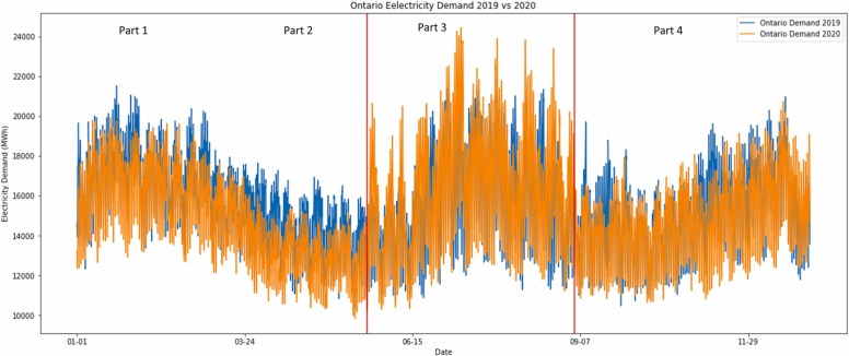
To give an overview of the changes in the hourly electricity demand in the year 2020 due to the pandemic, the demand data for both 2020 and 2019 are plotted against each other as illustrated in Fig. 1. The weekdays are aligned for both years to create an accurate comparative analysis between weekdays and weekends.

Fig. 1.

Ontario hourly electricity demand of the year 2019 against the year 2020 (The date displayed on the x-axis is considered for the year 2020, but the same weekdays are applied for both years).

Fig. 1 compares Ontario’s electricity demand for the years 2019 and 2020. As shown, the demand in the year 2020 has experienced different trend than 2019, which can be identified through 4 different intervals of time illustrated by the red vertical lines. For example, from the 3rd week of March after the essential business closure and until the 3rd week of May, the load dropped significantly compared to the load in 2019 as shown in part 2 Fig. 1. On the contrary, as shown in part 3, the load has unexpectedly experienced a high rise from the end of May until the beginning of September. Subsequently, the electricity demand in 2020 started to follow approximately the same normal shape as 2019. These three classifications of the electricity demand are going explained in detail in the next section with a profile of the monthly demand.

As shown in the first graph of Fig. 2, generally there are two common peaks throughout the day: morning and evening peaks, where the evening peak is much higher than the morning one. Beside the overall drop in the 2020 peak load, the morning and evening peaks also shifted. For example, in 2020 morning peak occurs later in the day and evening peak occurs earlier in the day than 2019. The reason for the changes in peak hours can be mainly due to the changes in individuals’ daily routines initiated by schools and business closure and working from home regulations implemented during COVID-19.

Fig. 2.

Electricity mean hourly demand and load duration curve 2019 vs 2020.

Lastly, the load duration curve is shown in the second graph of Fig. 2 to give an overall view of the cumulative hourly electricity demand for the year 2019 and 2020. The load duration curve is crucial in the electricity planning phase to identify the optimal capacity needed for generation. An annual load duration curve represents the load profile vs the time duration in hours where the load is arranged in a descending magnitudes order with the peak demand is the first point in the curve from the left. By reducing the peak demand, utilities can improve the efficiency of power generation (Alain et al., 2008). The second graph of Fig. 2 demonstrates the highest peak in 2020 surpasses 24,000 MW compared to 22,000 MW in 2019. On the other hand, the lowest peak is almost around 10,000 MW for both years, being slightly lower in 2020 which can be relevant to the decline that happened to the electricity demand in March and April due to the pandemic.

2.1.2. Monthly comparison of demand 2019 vs 2020

In this section the monthly electricity load is clustered into 3 categories as shown in Fig. 1 to present the reduction, the increase, and the recovery of the load between 2019 and 2020, as follows:

• a.From the first week of March until the third week of May.
• b.From the last week of May until the first Thursday of September.
• c.From the first Friday of September until the last week of December.

2.1.2.1. Monthly demand comparison: March to May

On March 12th Ontario's government announced the closure of schools, later on the 17th a state of Emergency was declared, followed by non-essential business closure on the 23rd (Nielsen, 2020). As a result of these fast-paced regulations implemented to reduce the risks of the COVID-19 spread, the energy consumption has witnessed a significant drop of almost 12% (IESO, 2020). This drop of load can be observed in the second part of Fig. 1.

2.1.2.2. Monthly demand comparison: May to September

As the weather became warmer and some businesses reopened, the electricity consumption started to ramp up once again by the mid of May. Consequently, towards the end of May, the demand of 2020 got significantly above 2019 demand rates. This phenomenon has been predominant in the period from the last week of May until the first few days of September as can be noticed in part 3 of Fig. 1. One reason for the high peaks in June 2020 is the Industrial Conservation Initiative (ICI) Hiatus that was announced to help large industrial consumers across Ontario recover from COVID-19 by focusing on higher production more than reducing their peak demand by reducing their electricity rates and minimizing their Global Adjustment costs ("Edgecom Energy,", 2020). In July 2020, the electricity demand jumped to its highest since July 17, 2013. Part of the demand increase in 2020 comparing to 2019 was due to hotter days. However, the weather did not have much impact on demand patterns as it was observed from the data. Overall, the recovery of the electricity demand in the summer exceeded the expectation of the Ministry of the Energy as well as the IESO ("Edgecom Energy,", 2020).

2.1.2.3. Monthly demand comparison: September to December

As COVID-19 cases started to rise in September, the government of Ontario decided to suspend the reopening plan on the 8th of September 2020 for a period of 4 weeks (Davidson, 2020). Therefore, as shown in part 4 of Fig. 1a decline in demand in September 2020 is evident. By the end of September, the load followed the same pattern as in 2019, which was consistent for the rest of the year, except for the first half of November, in which the demand declined, due to a rise in the around the 5th until almost the 20th of November 2020.

2.1.2.4. Mean hourly load based on months

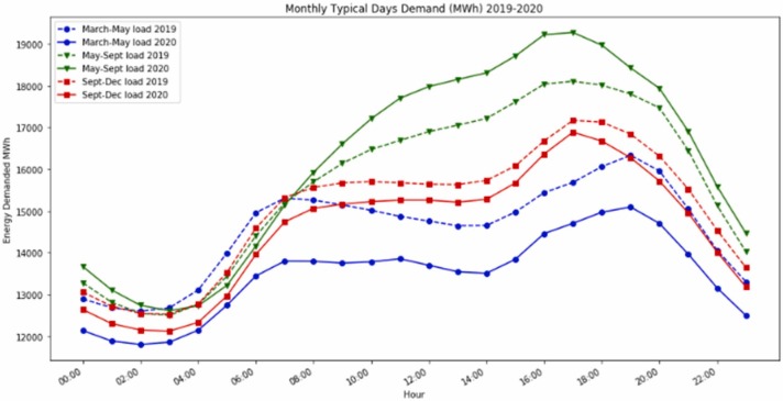
This section illustrates the hourly load for a typical day for the three classifications (March-May, May-September, September-December) mentioned in section II. A. 2) comparing 2019 and 2020. Fig. 3.

Fig. 3.

Mean hourly demand for each group of months for the years 2019–2020.

As shown, the difference between the representations of days for each group of months indicates load drop in March and April 2020 with a more flattened morning consumption due to the mandatory lockdown and working from home regulations. Also, an overall higher electricity demand is observed in the summer days of the year 2020, reaching its highest between 4 and 6 pm with delayed morning peaks and earlier evening peaks. The demand patterns are not changed between the years and months between 12:00–6:00 am, except March and April. Moreover, the lines representing the months from September to December are demonstrating the closest load patterns between 2020 and 2019, showing that the electricity demand nearly returned to normal behavior.

2.1.3. Daily comparison of demand 2019 vs 2020

This part compares the average hourly electricity demand for each day of the week, by evaluating the daily load profiles in 2020 and 2019. Also, to visualize this comparison in a general way, the daily demand is clustered, using K-means Clustering.

2.1.3.1. Weekdays mean hourly load

Fig. 4 displays 2 graphs of the mean hourly electricity demand for each day of the week for the years 2019 and 2020. By looking at the shown demand profiles, the general trends could be summarized as follow: the average morning and evening peaks were significantly higher in 2019, reaching around 19,000 MWh and over 20,000 MWh, respectively. Whereas in 2020 the maximum morning and evening peaks were around 17,000 MWh and over 18,000 MWh, respectively. Additionally, most of the weekdays demand pattern of 2020 are more converged and flattened than those of 2019.

Fig. 4.

Mean hourly energy demand for each day of the week 2019–2020.

Also as shown, the average energy consumption on the weekends is remarkably lower than the weekdays, especially in the morning and the afternoon, which can be expected due to schools and businesses normally functioning on weekdays. As for Sunday evenings, the demand ramps up getting closer to Fridays' load pattern, reaching an average of 18,500 MW/h. On the other hand, in 2020, the weekends are showing a slightly lower average electricity demand in the morning and the afternoon, with a peak on Sunday evenings almost the same as the weekdays, attaining more than 17,500 MW/h. This similarity could be the result of business closures and working from home mandates.

Finally, some distinctive trends can be noted for the different weekdays. For example, all the weekday curves of 2019 are adjacent except for Friday where the afternoon and evening energy profile is lower than the other weekdays. This variation can mostly be due to the fact that some businesses close earlier on Fridays. In 2020, the load profiles look different than usual, as the Mondays, Tuesdays, and Fridays average hourly consumption are closer to each other and more flattened than those of Wednesdays and Thursdays. Another noticeable trend is the presence of additional peak hours in the afternoon as can be seen on Tuesdays, Wednesdays, and Fridays. This fluctuation could be referred to the increase in residential electricity which mainly occurs between 11 am and 5 pm as customers are staying at home.

2.1.4. Daily K-means clustering of hourly loads

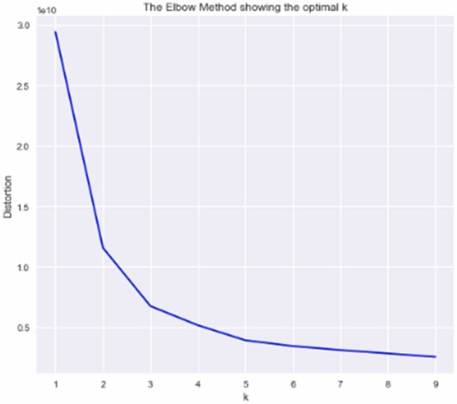
To dive deeper into the daily electricity consumption changes throughout, the K-means clustering algorithm is applied, using Scikit-Learn Python package (Viola, 2018). The data used for the clustering is starting from the first Sunday of March until the last Tuesday of December, which makes it 304 days (about 10 months) in total for each year. The optimal number of clusters was identified to be 3 clusters using the elbow method (Li, 2019) as shown in Fig. 5.

Fig. 5.

Elbow method.

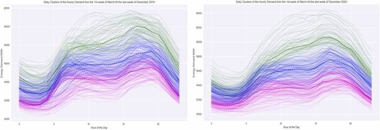
The resulted three clusters of daily demand profile are shown in Fig. 6. The green cluster represents the days with the highest peak load, while the blue and pink clusters represent days with moderate and base loads. Days with low demand could mainly be related to the mild-weather sunny days in both years, which is also confirmed by the March until May curve in Fig. 3.

Fig. 6.

Daily K-means clustering of hourly demand for the years 2019–2020.

2.2. Electricity supply impact analysis

Due to changes in demand, the supply of electricity in Ontario has changed accordingly, and therefore in this section an overview of changes in the supply sources of electricity is presented. The effect of changes in the supply mix on CO₂ emission is studied in the next section.

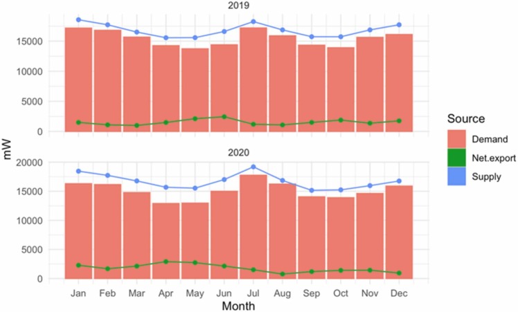
In Fig. 7, supply is strictly more than demand with the excessive amount is exported to other provinces or US. Both years exhibit a similar seasonality, reaching peak demand on January, July, and December.

Fig. 7.

Total Demand and supply of electricity in 2019 and 2020.

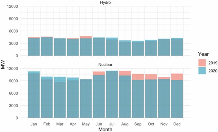
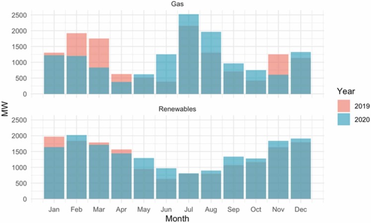
Most of the supply is provided by nuclear and hydro generators. Fig. 8 shows that the supply by hydro generators is closely similar between 2019 and 2020, as hydro capacities are used to satisfy the base load. However, nuclear and gas capacities are shown to generate slightly more in 2020 between January to April, while after the start of closure in Ontario, they supply less electricity. Lastly, it is important to note that the reduction in renewables supply seems to be covered by gas generators in February, March, and November. The supply by gas generators doubled in 2020 compared to 2019. Fig. 9.

Fig. 8.

Comparison between nuclear and hydro, 2019–2020.

Fig. 9.

Comparison between Gas and Renewables, 2019–2020.

3. Impacts of COVID-19 on the energy-related GHG emissions

To measure the impact of pandemic on GHG emissions in Ontario, the GHG intensity factor data ranging between January 2019 and December 2020 is used (Frommann and DiValentino, 2012). The data contains hourly energy production for each type of generator (i.e., Nuclear, Hydro, Gas, Solar, Wind, Biofuel, Other) in Ontario along with the GHG Intensity Emission Factor (EF), which is the ratio of total emission in grams of CO2 equivalent (gCO2eq) to the generated electricity (kWh), as follows:

$$E{F}_t=\frac{{\sum }_{i}CO{2}_{kt}}{P_{kt}}$$

for power plants $k\in \left[1,\dots ,\mathit{K}\right],$ where ${\mathit{CO}2}_{\mathit{kt}}$ and $P_{\mathit{kt}}$ are the total hourly emission (in grams) and electricity generated (in kWh) by generator $k$ at time t ( IPCC, 2006 ).

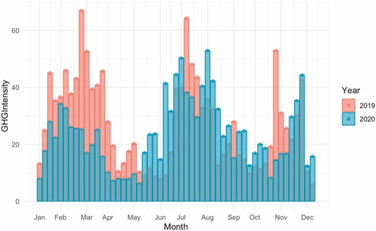
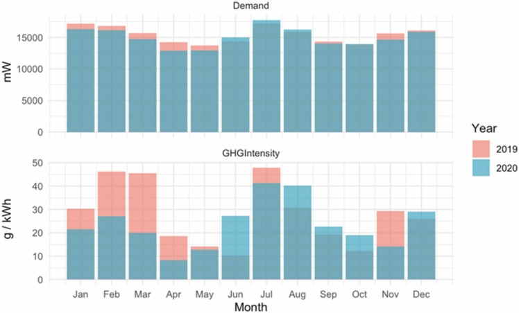
Fig. 10 presents the average hourly GHG Intensity factor described in Section II. As presented in the plot, GHG emissions are generally lower in 2020, with an overall 16.25% reduction. During the first five months of 2020, there is a significant difference between two years. This may be due to the first lockdown between March 17 and May 20. After the lockdown, however, the emissions are slightly higher compared to 2019, except for July and November.

Fig. 10.

GHG intensity by month.

The impact of the pandemic on GHG emissions is more severe, comparing to its impact on the electricity demand. As shown in Fig. 11, during the first five months of 2019, the GHG emission was approximately double its amount in 2020, indicating the impacts of industries closures.

Fig. 11.

Comparison between GHG and demand, 2019–2020.

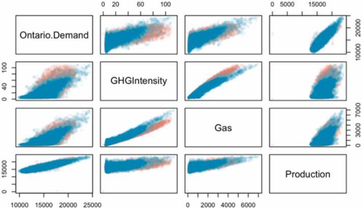
The positive correlation between demand and GHG emission is more evident for some generators rather than the others, as seen in Fig. 12. As shown, the linear relationship between GHG intensity and the production from gas generators imply that the main source of emission is the generated power from gas generators. Since the peak demand was reduced during pandemic, there was less need for the electricity production from gas generators and therefore the emission was reduced.

Fig. 12.

Pairs plot between demand, gas, GHG and total production.

The reduction in GHG emission cannot be significantly attributed to more renewable energy production, as there was approximately the same amount of renewable generation in 2019 and 2020, as shown in Fig. 9. The gas generators produced noticeably higher electricity between January to April and November in 2019, while their production was higher for the rest of the months in 2020.

4. Impacts of COVID-19 on load forecasting

Forecasting the electricity load is crucial for power system planning and operation. Understanding the impact of sudden events, such as COVID-19, on the electricity demand forecast is critical for policy makers. An accurate forecasting model becomes more challenging amidst the ongoing pandemic. Therefore, in this section the artificial intelligence (AI) models are studied for their prediction potentials in the presence of rare events.

4.1. Forecast model selection and structure

There are different types of forecast models that can be used to predict electricity demand; some are linear statistical models such as ARIMA and SARIMAX, and others are non-linear models, like neural networks. The comparison between the performance of the different types of forecast models are presented in (Kandananond, 2011) and (Pao, 2006), indicating better performance of Artificial Neural Network (ANN) compared to other linear methods. Neural Network models could learn complex non-linear relationships between the inputs and outputs whereas linear models, like SARIMAX, rely on more historical data (Shahriar et al., 2019) and (Singh et al., 2016).

In this paper, based on the electricity demand analysis, a load forecast Feed-Forward Neural Network (FFNN) model is chosen to consider different features, impacting the demand, such as seasons, days, hours, and weather. The related Ontario’s weather data, including temperature, wind direction, wind speed, and humidity, is obtained from Meteoblue’s historical data (Meteoblue, 2006–2021) and paired with Ontario’s demand data in the forecast model. The model provides comparisons of the resulted forecast between before and during pandemic.

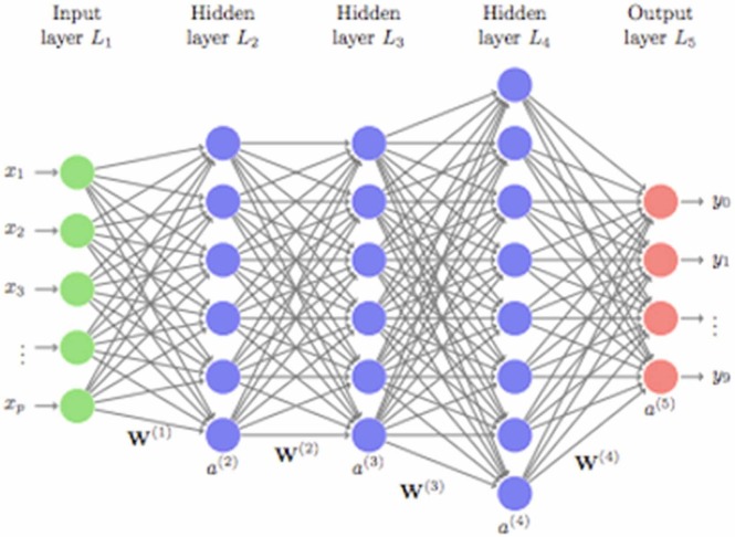
Fig. 13 shows a typical structure of a multi-layer FFNN model. The FFNN contains input data $\mathit{x}$ in input $l_1$, consisting of $\mathit{p}$ neurons, one or more hidden layer(s) $l_i$, for $i>0$ and an output of $y_i$, in output layer $l_n$, consisting of $\mathit{k}$ neuron(s). Each ${(i-1)}^{\mathit{th}}$ layer is fully connected to each $i^{\mathit{th}}$ layer with a coefficient matrix, $W^{(i)}$ for each layer $i$. Each neuron in the hidden layer(s) is activated using proper activation functions such as sigmoid and ReLU (Sharif and Taylor, 2000).

Fig. 13.

Feed forward neural network structure (Airforce Institute of Technology, 2021).

The data used for training the FFNN model consist of 27528 rows and 8 columns: date, time, hour, Ontario demand, temperature, humidity, wind speed, and wind direction, starting from the 1st of January 2018 until February 2021. The data is first examined for missing values, then more features are added to the data such as, the year, the season, the months, and the days to be used as input variables in the model. In order to find the relevant features for the analysis a feature selection method, considering the correlation between input and output layers is used.

In order to tune the model, different combinations of the number of layers, neurons, epochs, and batch sizes are examined. The best outcome is achieved with three hidden layers with 100 neurons, using ReLU activation function. Also, a subset of six predictors: temperature, humidity, wind speed, season, weekday, and hour yielded the best results. The network is trained with Adam optimizer to minimize the mean squared error between model predictions and output. The model is trained, using 100 epochs with batches of 10 data points in Python 3.7.12. and Tensorflow library with Keras interface.

Three separate models are trained for the time intervals, before and after the start of pandemic. The first interval (January 2018–January 2020) is to predict demand before the spread of the coronavirus, the second (January 2018–March 2020) is to study the performance of prediction methods during the lockdown, and the last interval (January 2018–January 2021) is to examine the impact of pandemic on prediction models after the stabilization of COVID-19 in 2021. The data is split such that there would be 15 days in each interval for test set and the rest used for training.

4.2. Forecast model performance and evaluation method

To evaluate the performance of the models, the Mean Absolute Percentage Error (MAPE) is calculated for each of the models to indicate the percentage of the error between the prediction and actual values for the training and testing datasets (Khair et al., 2017):

$$\mathit{MAPE}=\frac{1}{n}*\mathrm{\Sigma }\left(\frac{\left|A-F\right|}{\left|A\right|}\right)*100$$

Where, $n$ is the size of the sample, $A$ is the value of the actual data, and $F$ is the value of the forecast data.

4.2.1. . Model performance: pre-pandemic

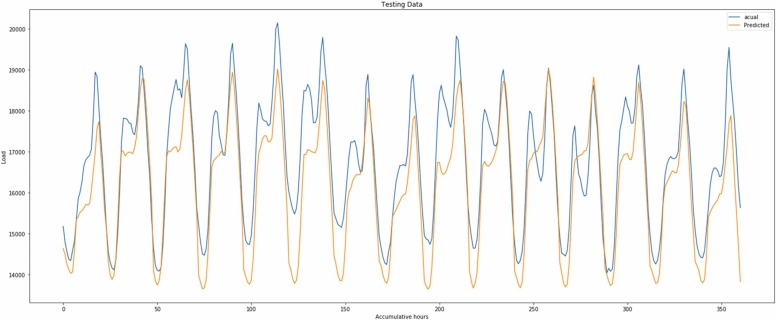
The pre-pandemic model is trained over pre-pandemic historical demand data (Jan 2018 – Jan 2020) and tested over pre-pandemic period of Jan 15, 2020 – Jan 29, 2020. As shown in Fig. 14 the performance of the test data in base case scenario is extremely accurate and has a MAPE = 3.21%.

Fig. 14.

Test data from Jan 15th, 2020, until Jan 29th 2020.

4.2.2. Model performance: beginning of pandemic

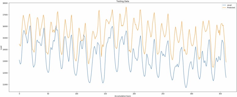
Next, a second model is trained using the same FFNN architecture, using training data (Jan 2018–March 2020), and then tested over the data in the beginning of pandemic, March 25, 2020–April 8, 2020. As shown in Fig. 15 and Table 1, the test performance declined significantly, due to the sudden changes in demand. The resulted MAPE during this period is 13.86%.

Fig. 15.

Test data from the 25th of March 2020 until the 8th of April 2020.

Table 1.

MAPE scores for the three models. The percentages in the table were rounded to 2 decimal places.

Models	Train data MAPE	Test data MAPE
Before the outbreak	6.58%	3.21%
During the outbreak	6.76%	13.86%
After the recovery	6.69%	4.23%

4.2.3. Model performance: during pandemic

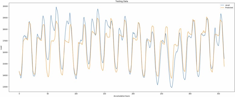
The FFNN model is retrained using the data from pandemic (Jan 2018–Jan 2021) and tested over the data from Jan 25, 2021–Feb 8, 2021, when the load behavior was stabilized. As seen in Fig. 16, the retained model, with the additional data from pandemic, performs with much higher accuracy of MAPE = 4.23%.

Fig. 16.

Test data from the 25th of Jan 2021 until the 8th of Feb 2021.

A summary of the error comparisons among the three models is given in Table 1. The results show good performance of the FFNN model, even during the beginning of. As noted in (Lewis, 1982), the evaluation of the accuracy of NN models, using MAPE can be categorized into 4 following categories in which the worst result of the proposed model is labeled as “good forecasting”:

• •Highly accurate forecasting if the MAPE < 10.
• •Good forecasting if the MAPE is between 10 and 20.
• •Reasonable forecasting if the MAPE is from 20 to 50.
• •And an inaccurate forecasting if the MAPE > 50.

4.2.4. Model Performance, using Cross Validation: beginning of pandemic

To examine, the model performance for the second model (beginning of pandemic) a cross validation on a rolling basis is used (Shrivastava, 2020). For this purpose, 5-folds cross validation technique is performed on the test data, while the training data is from January 1st, 2018, to March 15th, 2020, and the test data is from March 16th, 2020, until March 29th, 2020, for the first fold. For each of these intervals, the last test data points are then added as part of the training dataset and subsequent data points are included in the test data of the next fold. Finally, the average accuracy of the 5-fold cross validation is calculated. Table 2 illustrates each of the 5-fold intervals used, the accuracy of each fold, and the average accuracy for the overall cross validation performance.

Table 2.

Time series 5 folds cross-validation.

Folds	Training data	Test data	Accuracy (MAPE)
1	Jan 1, 2018– Mar 15, 2020	Mar 16, 2020–Mar 29, 2020	6.4
2	Jan 1, 2018–Mar 30, 2020	Mar 31, 2020–Apr 13, 2020	13.6
3	Jan 1, 2018–Apr 14, 2020	Apr 15, 2020–Apr 28, 2020	10.7
4	Jan 1, 2018–Apr 29, 2020	Apr 30, 2020–May 13, 2020	13.1
5	Jan 1, 2018–May 14, 2020	May 15, 2020–May 28, 2020	14.0
Average Accuracy (MAPE)			11.6%

As shown in the table, the main model here is represented by the 5th fold. The average accuracy presented by the cross-validation method is 11.6%, indicating higher accuracy than the MAPE error of 14%.

5. Conclusion & future work

In this paper, an extensive analysis of the COVID-19 impacts on Ontario’s electricity demand and supply has been performed including consequential GHG emissions and the complications that arise for accuracy of load forecasts in the presence of rare events. The additional complexity is addressed through use of the FFNN forecast model. The study showed significant load drop during March and April 2020 and unforeseen demand rise in the summer of 2020. In addition to a discussion on the changes in consumer’s behavior, the weather data was analyzed in detail shed light on the unexpected variations in demand. Also, the overall comparison between GHG emission and demand showed that the pandemic resulted in a significant reduction of GHG emissions during lockdown, when demand was lower than previous year. The study also showed noticeable increase in GHG emissions after the lockdown when the demand was higher than previous years. Through a detailed study, the relationship between demand and sources of generation, especially gas generation was illustrated. The paper also investigated the accuracy of forecasting methods before, beginning and during pandemic, and suggested that FFNN could result in good forecast of demand even in the beginning of pandemic.

In the future, this research will be extended to cater to scenarios for planning models that explicitly address unique rare events impacting the operation of electric grids, using insights gained in this study. Also, the changes in mobility, transportation, or employment data will be added to the proposed forecast model and tested for future improvement. Moreover, this research could be used as a benchmark to compare the Covid-19 pandemic to other rare events in the future.

Declaration of Competing Interest

The authors declare that they have no known competing financial interests or personal relationships that could have appeared to influence the work reported in this paper.

Biographies

Menna Elsarague is currently a master’s student at the Department of Management Sciences, at University of Waterloo. Her research focuses on applying data analytics tools to analyze the operations of electricity markets.

Mehrdad Pirnia is a faculty member at the Management Sciences Department, at University of Waterloo, where he is also cross appointed into the ECE Department. His research focuses on modeling and simulation of power and energy systems, using optimization, machine learning, and data analytics tools. He is particularly interested in the integration of renewable energy sources, storage capacities, and EVs to promote efficient energy policies to reduce GHG emission.

Fuat Can Beylunioglu is currently a Ph.D. student at the Department of Management Sciences, at University of Waterloo, where he also obtained his master’s degree. His research focuses on the theory of Neural Networks and applying machine learning techniques on power systems.

Mohamed Ahmed received the B.Sc. and M.Sc. degrees in electrical engineering from Ain Shams University, Cairo, Egypt, in 1999 and 2005, respectively, and the Ph.D. degree in electrical engineering from the University of Waterloo, Waterloo, ON, Canada, in 2012. From 2012–2014, he was a Senior Researcher with Smart-Planet Division, IBM Canada. From 2014–2015, he was a Technical Officer with Independent Electricity System Operator (IESO) of Ontario, Canada. From 2015–2018, he was a Senior Planning Engineer with SNC-Lavalin. He was the Lead Developer of the Demand Response Auction tool implemented in 2015 by IESO in Ontario. Since 2016, he has been an Assistant Professor with the Power and Machines Department, Ain Shams University, Cairo, Egypt, and an Adjunct Assistant Professor with the University of Waterloo, Waterloo, ON, Canada. He is also a Senior Specialist Energy Market, Market Power Mitigation with IESO. His research interests include electricity markets design, operation of power systems, distribution systems, reliability of electrical systems, power quality, active distribution systems, and power system optimization in the context of smart grids and microgrids.

Jatin Nathwani received the Ph.D. degree in engineering from the University of Toronto, Toronto, ON, Canada, in 1979. He was involved in a leadership capacity in the Canadian energy sector over a 30-year period. He brings a unique combination of academic perspectives with extensive experience in the business sector that includes corporate planning and strategy, energy sector policy reform, power system planning, environmental and regulatory affairs, and research program management. In 2007, he joined the University of Waterloo (UW), Waterloo, ON, Canada, where he is founded Waterloo Institute for Sustainable Energy (WISE), holding the prestigious Ontario Research Chair in Public Policy for Sustainable Energy. He serves on several boards at the provincial and national levels and has appeared frequently in the media (print, TV, and radio), having more than 100 publications related to energy and risk management, including seven books.

References

- Aburayash A., Dincer I. Analysis of the electricity demand trends amidst the COVID-19 coronavirus pandemic. Energy Res. Social Sci. 2020;68 doi: 10.1016/j.erss.2020.101682. [DOI] [PMC free article] [PubMed] [Google Scholar]
- Adeboye A., Bin Xu R. t E., Tamara a O. Covid-19 and the impact on energy consumption: an environmental assessment of Ontario Canada. Int. J. Sci. Res. Publ. 2020;10(8):2250–3153. [Google Scholar]
- Alain P., Michel D., Michaël F., Simon S. Load duration curve: a tool for technico-economic analysis of energy solutions. Energy Build. 2008;40(1):29–35. [Google Scholar]
- Alasali F., Nusair K., Alhmoud L., Zarour E. Impact of the COVID-19 pandemic on electricity demand and load forecasting. Sustainability. 2021;13(3):1435. [Google Scholar]
- Barooah, Agdas D., P Impact of the COVID-19 pandemic on the U.S. electricity demand and supply: an early view from data. IEEE Access. 2020;8:151523–151534. doi: 10.1109/ACCESS.2020.3016912. [DOI] [PMC free article] [PubMed] [Google Scholar]
- Airforce Institute of Technology, Data Science Lab R Programming Guide: Feedforward Deep Learning Models, Air Force Institute of Technology, (Online). 〈https://afit-r.github.io/feedforward_DNN〉. (Accessed 12 September 2021).
- S. Davidson, CTV News Toronto, Bell Media, 8 September 2020. (Online). 〈https://toronto.ctvnews.ca/ontario-forced-to-pause-reopening-plan-for-four-weeks-as-covid-19-cases-spike-1.5095876〉. (Accessed 16 February 2021).
- Edgecom Energy, Edgecom Energy Inc 2020, 11 January 2021. (Online). 〈https://www.edgecomenergy.ca/resources1/the-industrial-conservation-initiative-is-coming-back-in-may-2021〉. (Accessed 15 February 2021).
- Frommann K., DiValentino E. Calculation and application of hourly emission factors for increased accuracy in scope two emission calculations. Trans. Canadian Soc. Mech. Eng. 2012;36(2):143–148. [Google Scholar]
- IESO, IESO News: COVID-19 impacts on Ontario's electricity system. Independent Electricity System Operator, 30 April 2020. (Online). 〈https://ieso.ca/en/Sector-Participants/IESO-News/2020/04/COVID-19-impacts-on-Ontarios-electricity-system〉. (Accessed 3 June 2020).
- IPCC, Stationary combustion, In: Guidelines for National Greenhouse Gas Inventories, 2006, 2.13.
- Jiang P., Fan Y.V., Klemeš J.J. Impacts of COVID-19 on energy demand and consumption: Challenges, lessons and emerging opportunities. Appl. Energy. 2021;285 doi: 10.1016/j.apenergy.2021.116441. [DOI] [PMC free article] [PubMed] [Google Scholar]
- Kandananond K. Forecasting electricity demand in Thailand with an artificial neural network approach. Energies. 2011;4(8):1246–1257. [Google Scholar]
- Kentaka Aruga, Islam, Jannat M., Arifa a. Effects of COVID-19 on Indian energy consumption. Sustainability. 2020;12(14):5616. [Google Scholar]
- Khair U., Fahmi H., Al Hakim S., Rahim R. Forecasting error calculation with mean absolute deviation and mean absolute percentage error. J. Phys. Conf. Ser. 2017;930(1) [Google Scholar]
- Lewis C. Butterworths; London: 1982. Industrial and Business Forecasting Methods. [Google Scholar]
- L. Li, Towards Data Science: K-Means Clustering with scikit-learn, Medium, 30 May 2019. (Online). 〈https://towardsdatascience.com/k-means-clustering-with-scikit-learn-6b47a369a83c〉.
- , Meteoblue, WeatherToronto, Meteoblue Weather, 2006-2021. (Online). 〈https://www.meteoblue.com/en/weather/archive/export/toronto_canada_6167865〉.
- K. Nielsen, Global News, A timeline of COVID-19 in Ontario, Corus, 24 April 2020. (Online). 〈https://globalnews.ca/news/6859636/ontario-coronavirus-timeline/〉. (Accessed 2 November 2020).
- Pao H.-T. Comparing linear and nonlinear forecasts for Taiwan’s electricity consumption. Energy. 2006;31(12):2129–2141. [Google Scholar]
- Shahriar M.S., Hasan K.M., Abrar Al, S. R An effective artificial neural network based power load prediction algorithm. Int. J. Comput. Appl. 2019;178(20):0975–8887. [Google Scholar]
- S.S. Sharif , J.H. Taylor, Short-term load forecasting by Feed forward neural networks, in: Proceedings of the IEEE ASME First Internal Energy Conference (IEC), Al Ain, United Arab Emirate, 2000.
- S. Shrivastava, medium, medium, 14 Jan 2020. (Online). 〈https://medium.com/@soumyachess1496/cross-validation-in-time-series-566ae4981ce4〉. (Accessed February 2021).
- N.K. Singh, A.K. Singh ,N. Paliwal, Neural Network based short-term electricity demand forecast for Australian states, in: Proceedings of the IEEE First International Conference on Power Electronics, Intelligent Control and Energy Systems (ICPEICES), IEEE, 2016.
- L.G. Viola, Towards Data Science, Medium, 17 Sept 2018. (Online). 〈https://towardsdatascience.com/clustering-electricity-profiles-with-k-means-42d6d0644d00〉. (Accessed 15 October 2020).
- World Health Organization, Statement on the Second Meeting of the International Health Regulations (2005) Emergency Committee Regarding the Outbreak of Novel Coronavirus (2019-nCoV) 30 January 2020. (Online). 〈https://www.who.int/news/item/30–01-2020-statement-on-the-second-meeting-of-the-international-health-regulations-(2005)-emergency-committee-regarding-the-outbreak-of-novel-coronavirus-(2019-ncov)〉. (Accessed 15 August 2020).