Abstract
The lockdown measures in response to the SARS-CoV-2 virus outbreak in 2020 have resulted in reductions in emissions of air pollutants and corresponding ambient concentrations. In the Netherlands, the most stringent lockdown measures were in effect from March to May 2020. These measures coincided with a period of unusual meteorological conditions with wind from the north-east and clear-sky conditions, which complicates the quantification of the effect of the lockdown measures on the air quality. Here we quantify the lockdown effects on the concentrations of nitrogen oxides (NOx and NO2), particulate matter (PM10 and PM2.5) and ozone (O3) in the Netherlands, by analyzing observations and simulations with the atmospheric chemistry-transport model EMEP/MSC-W in its EMEP4NL configuration, after eliminating the effects of meteorological conditions during the lockdown. Based on statistical analyses with a Random Forest method, we estimate that the lockdown reduced observed NO2 concentrations by 30% (95% confidence interval 25–35%), 26% (21–32%), and 18% (10–25%) for traffic, urban, and rural background locations, respectively. Slightly smaller reductions of 8–28% are found with the EMEP4NL simulations for urban and regional background locations based on estimates in reductions in economic activity and emissions of traffic and industry in the Netherlands and other European countries. Reductions in observed PM2.5 concentrations of about 20% (10–25%) are found for all locations, which is somewhat larger than the estimates of 5–16% based on the model simulations. A comparison of the calculated NO2 traffic contributions with observations shows a substantial drop of about 35% in traffic contributions during the lockdown period, which is similar to the estimated reductions in mobility data as reported by Apple and Google. Since the largest health effects related to air pollution in the Netherlands are associated with exposure to PM10 and PM2.5, the lockdown measures in spring of 2020 have temporarily improved the air quality in the Netherlands. The concentrations of the most health relevant compounds have only been reduced by about 10–25%.
Keywords: Nitrogen dioxide, Particulate matter, Covid-19, Random forest, Ozone
Graphical abstract
1. Introduction
Concentrations of most air pollutants have decreased significantly in the past decades in most countries in Europe as a result of various policy measures, but current levels are still responsible for significant adverse health effects (EEA, 2019; Velders et al., 2020). The lockdown measures in Europe in response to the corona SARS-CoV-2 virus outbreak, causing COVID-19 disease, have significantly reduced traffic volumes and industrial activities in 2020. As a direct result, emissions of various air pollutants from these sectors have also been reduced, although the magnitude of the reductions has not been assessed yet. Satellite observations of nitrogen dioxide (NO2) of China, Northern Italy, and the USA have shown reductions in column densities in spring of 2020 which are attributed to the corona lockdown measures in these countries (Bauwens et al., 2020; Liu et al., 2020). Shi and Brasseur (2020) analysed more than 800 monitoring sites in northern China and derived decreases in PM2.5 and NO2 surface concentrations of 35% and 60%, respectively, during the lockdown. Cole et al. (2020) applied a machine learning technique to observations in Wuhan (China) to remove the effects of weather patterns and an augmented synthetic control approach to compare cities with and without a lockdown. They found a reduction in concentrations of about 60% for both NO2 and PM10 in Wuhan. Giani et al. (2020) combined observational data with simulations with a chemistry-transport model and reported reduced PM2.5 concentrations in China and Europe and the averted short- and long-term mortality from air pollution due to the lockdown.
Quantifying the effects of the lockdown measures in terms of reductions in concentrations, e.g., of NO2 and particulate matter (PM10, PM2.5), is not trivial and requires a separation of these effects with those from natural variability driven mostly by meteorological conditions. The Netherlands experienced unusual meteorological conditions in spring 2020 starting at about the same time as the corona lockdown measures; from the middle of March till the beginning of May 2020 there was more sunshine than the long-term average, as well as dry conditions and a long period with a sustained wind from the east and north-east bringing in air from Germany and eastern Europe to the Netherlands. These unusual meteorological conditions affect the concentrations of air pollutants and make it challenging to identify and quantify the effects of the lockdown measures on the concentrations.
Three methods are employed here to quantify the effects of the lockdown measures on the concentrations of NO2, NOx, PM10, and PM2.5, and O3 in the Netherlands. First, we report on the observed trends in surface concentrations from various measurement stations in the Netherlands from January till May 2020 and use a machine learning algorithm (Random Forest method (Breiman, 2001; Tong et al., 2003)) to estimate what the concentrations in spring 2020 would have been without the lockdown measures. Second, we performed simulations with the atmospheric chemistry-transport model EMEP/MSC-W (Simpson et al., 2012) in its EMEP4NL configuration (Van der Swaluw et al., 2020) using a reference scenario and scenarios with estimates of emission reductions to disentangle the effects of the corona lockdown measures on concentrations from those caused by meteorological variability. Third, reductions in the traffic NO2 contribution are determined by comparing observed concentrations in streets with reported traffic data.
The following sections present the measurement networks, the statistical method employed, a concise description of the EMEP4NL simulations, the trends in observed trends in NOx, NO2, PM10, PM2.5 and O3, the results of the model simulations, and a discussion and conclusions.
2. Methods
2.1. Air quality measurement networks
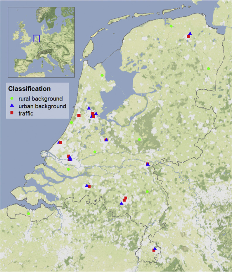
Air quality measurements in the Netherlands are performed by the National Air Quality Monitoring Network (LML, 2020) of the National Institute for Public Health and the Environment (RIVM), the DCMR Environmental Protection Agency (DCMR, 2020), and the Public health department of Amsterdam (GGD, 2020). Measurements have been used of the hourly average NOx, NO2, PM10, PM2.5, and O3 concentrations at rural backgrounds, urban backgrounds, and in city streets (traffic locations), in the Netherlands. Data from continuous measurements from January 2017 through May 2020 with high data coverage have been used of NOx and NO2 from 34 stations, PM10 from 29 stations, PM2.5 from 26 stations, and O3 from 23 stations. Stations were selected across the country, were several compounds are measured simultaneously and were traffic and urban background stations are at close proximity. This set consists of 9 rural background stations, 11 urban background stations, and 14 traffic stations (see Fig. 1 and Appendix A; Tables A1 to A5).
Fig. 1.
Location of the monitoring stations used in this study (Map tiles by Stamen Design, under CC BY 3.0. Data by OpenStreetMap, under ODbL).
2.2. Back trajectories
The Hybrid Single-Particle Lagrangian Integrated Trajectory (HYSPLIT) model was used to calculate hourly back-trajectories of air parcels during the lockdown period (Draxler and Hess, 1998). Using the HYSPLIT model, a single air parcel is followed originating from the receptor site backwards in time for 24 h. Backward trajectories have been calculated for every hour in the lockdown period. These trajectories provide information about the origin of an air parcel during a specified period. Meteorology from the Global Data Assimilation System at a resolution of 1 × 1 degree (GDAS1) is used with a starting height of 10 m above ground level at the receptor site. The time interval was 1 h, and the model height, setting the vertical limit of HYSPLIT model calculations, was set to 10 km. A simple approach was used to determine the prevalent wind sectors for the lockdown period. This approach consisted of calculating the proportion of the time a particular air parcel (i.e., trajectory) resided in various wind sectors (Carslaw and Ropkins, 2012). A wind sector was assigned to each of the hourly back trajectories if the air parcel spends at least 13 of the 24 h in that sector. The same method was also used for the defined period in 2017, 2018, and 2019.
2.3. Statistical analyses of the air quality data with Random Forest
Machine learning algorithms are being used increasingly to forecast atmospheric concentrations (Alimissis et al., 2018; Feng et al., 2018; Lautenschlager et al., 2020). Here the Random Forest machine learning algorithm (Breiman, 2001; Tong et al., 2003) is used to separate the effects of the meteorological variability on the air pollutant concentrations from that of the lockdown measures. A Random Forest method can handle the nonlinear relationship between various parameters and concentrations (Grange and Carslaw, 2019). The R software package “rmweather” (Grange, 2018) was used for the Random Forest method. First, a Random Forest model is constructed with the following explanatory variables: day of the year, day of the week, hour of the day, local temperature, precipitation, wind direction, wind speed, air pressure, humidity, global radiation, and cloud cover. For the meteorological parameters, data from the Royal Netherlands Meteorological Institute (KNMI, 2020) was used. Continuous measurements of various meteorological variables are collected from approximately 45 automatic weather stations in the Netherlands. Not all selected parameters are measured at each weather station. Hence, each meteorological parameter was attached independently based on proximity, choosing measurements from the nearest available weather station with the highest data capture. Second, the Random Forest explanatory variables are determined using a training dataset consisting of all hourly observations from January 1, 2017 to February 29, 2020. This is performed for each measurement station and compound separately. Third, the method is then used to estimate expected hourly pollutant concentrations based on the meteorological circumstances and other explanatory variables under the assumption that emissions are as business-as-usual, i.e., there was no lockdown. This is performed for each measurement location before and during the lockdown period, until the end of May 2020. Fourth, the concentrations that are measured before and during the lockdown period are compared with the “expected” concentrations during this period. The difference between observed and expected concentrations are ascribed to the lockdown measures. Finally, the station-specific mean differences between daily observed and expected concentrations during the lockdown period, and their corresponding confidence intervals, are pooled using a random-effects meta-analysis per station type (traffic location, urban background, or rural background) using the R metafor package (Viechtbauer, 2010). The results from the individual stations are combined per station type. Because of differences between the measurement stations (e.g., location, local contribution of emission sources, equipment) we assume variability (heterogeneity) among the individual results. In a random-effects model this heterogeneity is treated as purely random. The variance between stations is estimated from the data and used to modify the weights in the calculation of the random-effects summary estimate (DerSimonian and Laird, 1986). Here, the summary estimate is calculated as an overall mean difference between the observed and expected concentrations, and therefore an indication of the nationwide effect of the lockdown measures on concentrations.
2.4. EMEP4NL model and scenarios
Model simulations are performed using scenarios of emission reductions from the lockdown measures and the Eulerian grid model EMEP/MSC-W (Simpson et al., 2012) for the Netherlands in its EMEP4NL configuration (Van der Swaluw et al., 2020) to estimate the effects of the lockdown on the concentrations in the Netherlands. The EMEP model has been extensively validated for Europe (EMEP, 2020) and for individual countries such as the Netherlands (EMEP/MSC-W, 2020). The EMEP model (version rv4.33) is used with nested grids to obtain a resolution of 1.3 × 2.1 km over the Netherlands. The model is run offline with the meteorological data from the Weather Research Forecast (WRF, NCAR (2020)) model (version 3.8). The official 2014 EMEP emissions, gridded with the TNO-MACC III spatial distribution (Kuenen et al., 2014; MACC, 2016), is scaled with emissions from the European Centre on Emission Inventories and Projections (CEIP, 2020) for the different countries and 10 SNAP (Selected Nomenclature for Air Pollution) sectors to represent emission for the year 2016. Detailed Dutch emissions (see, e.g., Hoogerbrugge et al. (2019)) are used for the same reference year for the highest grid-level over the Netherlands.
Two sets of model simulations are performed: 1) simulations with three lockdown scenarios, with reduced emissions corresponding to the lockdown measures, and meteorology from January to May 2020, 2) simulations with a reference scenario with emissions corresponding to the year 2016 and meteorology from January to May of 2017, 2018, 2019, and 2020 to study the effects of the meteorology on the pollutants concentrations. Since we are interested in concentration differences between the scenarios, the absolute values of the emissions, i.e., for the year 2016, used in the simulations are not so important.
The magnitude of the emission reductions caused by the lockdown has not been assessed yet by the national reporting organizations, such as the Dutch Pollutant Release and Transfer Register (PRTR, 2020) and CEIP (2020). The lockdown scenario, therefore, consists of a low and high scenario with estimated reductions in emissions in the 10 SNAP sectors for each country in Europe (Table 1 ). Reductions are estimated for the transport sector, mainly passenger cars, and for industrial sectors. The reductions are not the same for all countries. We assumed a somewhat smaller reduction for countries with a partial lockdown, such as the Netherlands, Belgium, and Germany, and larger reductions for countries with a more stringent lockdown, such as France, Italy, Spain, and the United Kingdom. A third scenario, called extended lockdown scenario, is defined with reductions in emissions larger than estimated based on reported reductions in economic activities. Since the reported reductions in economic activities are based on a limit number studies and proxy data for activities of specific sectors, the extended lockdown scenario is probably an upper limit, but still possible scenario.
Table 1.
Reductions in emission applied to the various sectors in the low, high, and extended lockdown scenarios.
| Industrial sector (SNAP codes) |
Netherlands, Belgium, Germanya |
France, Italy, Spain, UKb |
||||
|---|---|---|---|---|---|---|
| low | high | extf | Low | high | extf | |
| 1. Combustion energy industriesc | 5% | 15% | 25% | 20% | 30% | 40% |
| 2. Non-industrial combustion | – | – | – | – | – | – |
| 3-6. Industrial combustion and production processesd | 5% | 15% | 25% | 20% | 30% | 40% |
| 7. Road transporte | 20% | 40% | 60% | 30% | 50% | 70% |
| 8. Other mobile sources and machineryd | 5% | 15% | 25% | 20% | 30% | 40% |
| 9. Waste treatment and disposal | – | – | – | – | – | – |
| 10. Agriculture | – | – | – | – | – | – |
Countries with a partial lockdown include the Netherlands, Austria, Belgium, Denmark, Finland, Germany, Luxembourg, Norway, Sweden, and Switzerland.
Countries with a stringent lockdown include, France, Ireland, Italy, Spain, and the United Kingdom.
A reduction in electricity production of 5–10% is reported for the Netherlands (PBL, 2020; Tennet, 2020). IEA (2020) reported a reduction in electricity demand of 10% for Germany. Larger reductions are reported for countries with a stricter lockdown, i.e., 20% for France and Spain, 16% for the United Kingdom and 37% for Italy (IEA, 2020).
For the Netherlands, the daily industrial production was reported to be 11% lower in April 2020 than in April 2019 (CBS, 2020). A larger reduction is assumed for countries with a stringent lockdown in line with the reductions in electricity demand (note c). The same reductions are applied to SNAP 8 (Other mobile sources).
KIM (2020a) reported reductions in total traffic of 39% on highways and 32% on other roads, while reductions of only 7–8% are reported for heavy duty transport. NDW (2020) measurements of traffic volumes on highways in the Netherlands show reductions of 40–60% for passenger cars and much smaller reductions for heavy duty transport. Based on this we assume for the low and high scenarios an average reduction in emissions for all traffic (passenger cars, light and heavy-duty transport) on motorways and other roads of 20–40% for the Netherlands countries with a similar lockdown and 30–50% for other countries.
For the extended lockdown scenario larger reductions in emissions are assumed than based on the reported reductions in economic activities.
The reductions from Table 1 are applied to all the emissions of a sector in a country; no spatial differentiation in the reductions in a country is applied. No reductions are assumed for the emissions from buildings, waste disposal and treatment, and agriculture. There are no indications that the number of animals on farms changed during the lockdown and therefore the agricultural emissions are assumed not to be affected by the lockdown.
2.5. Model calculations local traffic contributions
As part of the air quality monitoring in the Netherlands, detailed hourly maps of NO2 and PM10 concentrations are calculated by RIVM (2020). These maps are based on estimated real-time hourly background concentrations calculated using the RIO model (Residual Interpolation optimised for Ozone (Janssen et al., 2008)). A Gaussian dispersion model is used to add local traffic contributions for locations within a radius of 5 km from all significant roads and highways in the Netherlands. These calculations use observed meteorological conditions and estimated traffic emissions, specific for the hour and day of the week (Wesseling and Van Velze, 2014).
The calculated hourly concentrations are combined with the available NO2 and PM10 measurements in the Netherlands (see section 2.1) to calculate the difference (bias) between the maps and measurements at background locations. Furthermore, the calculated and measured concentrations near roads are used to estimate a scaling factor for the assumed traffic emissions. Under normal conditions, the bias is, on average, zero and the scaling factor of the traffic emissions is approximately 1. During periods with reduced traffic, such as during the lockdown period, the scaling factor of the traffic emissions drops below 1. In 2020, the observed prolonged period with scaling factors below 1 (indicating lower traffic emissions than usual) is attributed to the effects of the lockdown measures, although other factors can play a role as well.
The scaling factors are compared with the data provided by Apple (2020) and Google (2020). The Apple data is based on “a relative volume of directions requests per country/region, sub-region or city compared to a baseline volume on 13 January 2020”. We have used the average value of the categories “driving” and “transit”. Google provides, among others, the categories “Mobility trends for places like public transport hubs such as subway, bus, and train stations” and “Mobility trends for places of work”. The average of these categories is used here.
3. Results
The lockdown period is not precisely defined and varies for different countries. Traffic data from Apple (2020) and Google (2020) show a considerable reduction in traffic intensity, starting mid-March in most countries in Europe after which the intensity gradually increased and returned to close to ‘normal’ values by mid-June. For the present study, the lockdown period is defined as a period of eight weeks starting at March 16, 2020, when the schools in the Netherlands closed and people were asked to work from home, and ending May 10, 2020, when the primary schools opened again. For this period, the reductions in observed concentrations (sections 3.3) are determined as well as in modelled concentrations (section 3.4). First, the meteorology in the Netherlands during the lockdown period is discussed (section 3.1) and the trends in observed concentrations (section 3.2). The reduction in traffic intensity is estimated in section 3.5.
3.1. Meteorology during the lockdown
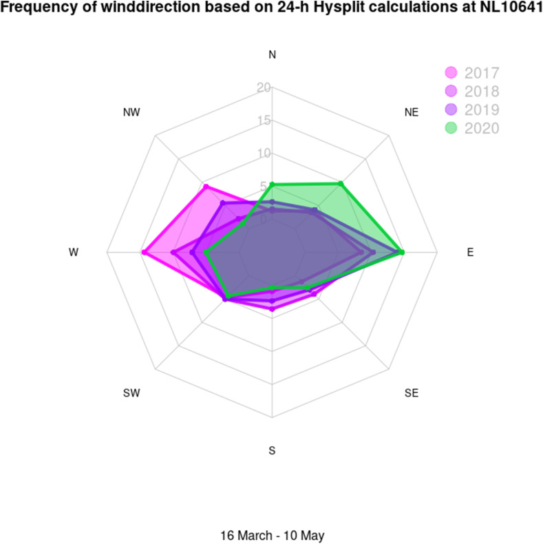
The meteorology during the lockdown has a significant effect on concentrations, especially wind direction and precipitation. The prevailing wind directions from 2017 to 2020 have been calculated using hourly air mass back trajectories for the entire lockdown period for station Breukelen (see section 2.2). This air quality station is situated in a mostly rural area in the centre of the Netherlands, near a major highway between Amsterdam and Utrecht. In Fig. 2 (and Appendix A, Fig. A.1) the prevalent wind sectors for Breukelen in 2020 during the lockdown period are compared with the prevalent wind sectors from previous years. During the lockdown period, the back trajectory analysis shows that the wind in the Netherlands came predominantly from the east and north-east. In contrast, in preceding years the winds came more from the west during the corresponding period of each year. Wind from especially the south-east generally lead to higher concentrations of air pollutants in the Netherlands, often because of stable and dry meteorological conditions and long-range transport of pollutants from Eastern Europe to the Netherlands.
Fig. 2.
Prevailing wind directions in the centre of the Netherlands (measurement station Breukelen) during the lockdown period (March 16 to May 10, 2020) and the winds in the corresponding period in 2017, 2018, and 2019. See Appendix AFig. A1 for the wind directions averaged over two-week periods.
Furthermore, the lockdown period was dry and sunny, with only 24 mm of precipitation versus 97 mm as climatological average and 513 h of sunshine versus 304 normal in the centre of the Netherlands (weather station De Bilt (KNMI, 2020)). The diurnal average temperature was close to normal (9.9 °C versus 9.0 °C climatologically).
3.2. Trends in observed concentrations
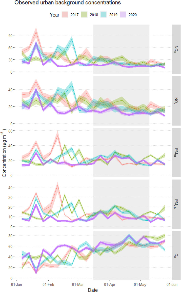
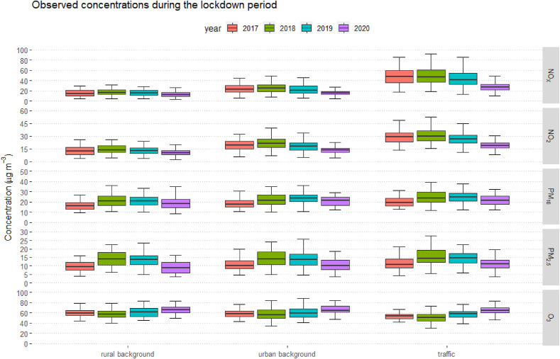
The concentrations of air pollutants show large variability on an hourly and daily basis, mostly as the result of meteorological variability. To easier compare the observed concentrations for different years, the variability is reduced by calculating weekly average concentrations. The trend in observed weekly average concentrations of NOx, NO2, PM10, PM2.5, and O3 are shown in Fig. 3 for the average of urban background locations. The 2020 data is compared with data for the same period in 2017, 2018, and 2019. See Appendix A (Fig. A2 and Fig. A3) for the corresponding figures for rural background and traffic locations. The concentrations averaged over the whole lockdown period for 2017 to 2020 are presented in Fig. 4 .
Fig. 3.
Observed weekly average urban background concentrations of NOx, NO2, PM10, PM2.5, and O3 for the period January to May for 2017 to 2020. The shared areas around the lines show the 95% confidence interval. The grey shaded region shows the lockdown period. The dates correspond to the start of the week.
Fig. 4.
Statistics of the observed concentrations of NOx, NO2, PM10, PM2.5, and O3 during the lockdown period for 2017 to 2020. Shown are the median, 25 and 75 percentiles and minimum and maximum concentrations.
The 2020 NOx and NO2 concentrations are mostly below the corresponding concentrations in 2017–2019 already before the lockdown period, at the rural and urban background and traffic locations. Low 2020 concentrations are observed in February, before the lockdown, probably because of sustained winds and rain. The 2020 concentrations are more or less constant from the beginning of February till the end of May and do not show a decrease during the lockdown period. PM2.5 and PM10 show low concentrations in February and beginning of March, mostly lower than the corresponding values in 2017–2019. The 2020 concentrations increased in the middle of March when the lockdown measures started. During the lockdown period, the average 2020 PM2.5 and PM10 concentrations are somewhat lower than in the years 2017–2019. Ozone concentrations show a different trend. They clearly increased towards spring and summer as ozone production increases as the amount of sunlight (UV-radiation) increases in combination with stable weather conditions. The 2020 O3 levels are mostly higher than the concentrations in the corresponding period in 2017–2019.
Comparing the 2020 concentrations averaged over the lockdown period with those of the previous years (Fig. 4) shows that the 2020 concentrations are for most compounds and station types not very different from the that in the previous years. The 2020 concentrations at the traffic stations show the largest difference with the previous years, but even for these the 95% confidence intervals mostly overlap. This shows that a direct comparison of the 2020 trends with those in the previous years is not sufficient to estimate the effect of the lockdown measures on the air quality. In section 3.3 we discuss the use of a machine learning algorithm to separate and quantify the effects the lockdown measures on the concentrations from those of the meteorological variability.
3.3. Lockdown effect on observed concentrations
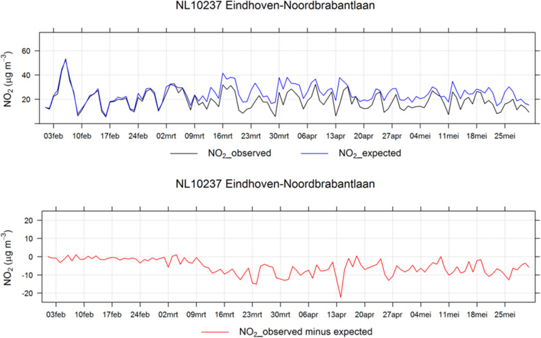
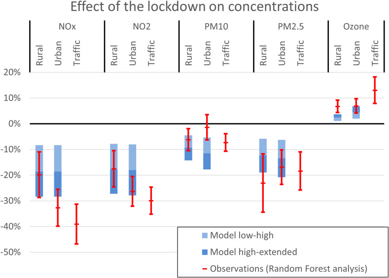
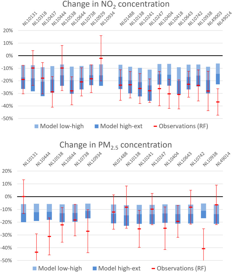
A Random Forest method (see section 2.3) is used to obtain expected concentrations of air pollutants, i.e., concentrations under the current meteorological conditions with business-as-usual emissions, at each measurement location (section 2.1) for the lockdown period in 2020. Fig. 5 shows an example of the expected concentrations of NO2 for a single measurement station together with the observed concentration. The difference between the observed and expected concentration is ascribed to the lockdown measures. The observed NO2 concentration at this station drops below the expected concentration at the beginning of March and stays there for the next months, although with considerable variability. Fig. 6 shows the average reduction in concentration for the different pollutants and different types of stations. In Fig. 8 and Fig. A4 the reductions and confidence intervals for individual stations are shown. See Appendix A (Tables A1 to A5) for the average concentrations of all compounds during the lockdown period for all measurement locations individually.
Fig. 5.
Daily average observed and expected NO2 concentration for February to May 2020 (top panel). The expected concentration is estimated using a Random Forest method and represents the concentrations corrected for meteorological variability. Also shown (bottom panel) is the difference between the observed and expected concentration, which is an indication of the effect of the lockdown measures on the concentration.
Fig. 6.
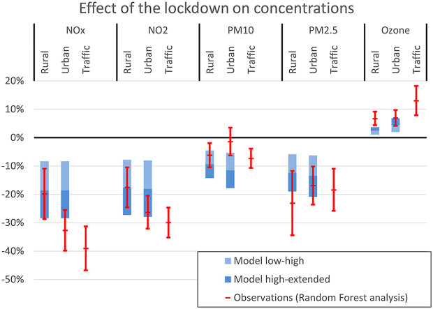
Effect of the lockdown measures on the NOx, NO2, PM10, PM2.5 and O3 concentrations based on the Random Forest analyses (red lines, labelled ‘Observations’) and EMEP4NL scenario calculations (blue bars, labelled ‘Model’). Shown are the effects for rural, urban, and traffic measurement locations, averaged over de lockdown period. The EMEP4NL results show the difference between the reference scenario and the three lockdown scenarios with low, high, and extended emissions reductions. Because of the spatial resolution of 1.3 × 2.1 km the EMEP4NL simulations are not suitable to calculate concentrations at traffic locations. The light blue band show the low to high scenario and the dark blue band the high to extended scenario. The Random Forest results show the difference between the expected concentrations, without lockdown measures, and the observed 2020 concentrations. The vertical lines are the 95% confidence intervals. (For interpretation of the references to colour in this figure legend, the reader is referred to the Web version of this article.)
Fig. 8.
Effect of the lockdown measures on the NO2 and PM2.5 concentrations based on the Random Forest analyses (red lines, labelled ‘Observations’) and EMEP4NL scenario calculations (blue bars, labelled ‘Model’). The bars show the difference between the lockdown scenarios and the reference scenario, averaged over March 16 to May 10, 2020. The light blue band show the low to high scenario and the dark blue band the high to extended scenario. The Random Forest results show the difference between the expected concentrations, without lockdown measures, and the observed 2020 concentrations. The vertical lines are the 95% confidence intervals. The stations on the left (9 for NO2 and 6 for PM2.5) are rural background stations and those on the right (11 for NO2 and 9 for PM2.5) are urban background stations. (For interpretation of the references to colour in this figure legend, the reader is referred to the Web version of this article.)
The largest reductions during the lockdown period are found for the NOx concentrations at traffic locations, on average, 39%, with a 95% confidence interval (CI) of 31–47%. The reduction at urban background locations is 33% (95% CI 25–40%) and at rural background locations is 20% (95% CI 11–29%). Slightly smaller reductions are found for NO2 concentrations with on average 30% (95% CI 25–35%), 26% (95% CI 21–32%), and 18% (95% CI 10–25%) for traffic, urban, and rural background locations, respectively. The large decreases in concentration at traffic locations indicate that the reductions in traffic volume and emissions play an important role.
The reductions in PM2.5 concentrations during the lockdown period are smaller than those of NOx and NO2, and about the same at all types of measurement locations; on average about 20% (95% CI 10–25%). The reductions in PM10 are just statistically significant at all stations, with an overall reduction of about 5% (95% CI 0–10%). PM2.5 and PM10 show smaller spatial gradients in the Netherlands than nitrogen oxides since they originate from both primary and secondary emissions (see section 3.4).
Statistically significant overall increases are found for O3 concentrations for all station types, but especially for traffic locations. Increases in O3 are a direct result of decreases in NOx emissions and NO concentrations through reduced ozone titration. On average, O3 increases by 13% (95% CI 8–18%), 7% (95% CI 4–10%), and 7% (95% CI 4–9%) for traffic, urban, and rural background locations, respectively.
3.4. Modelled effect of lockdown on concentrations
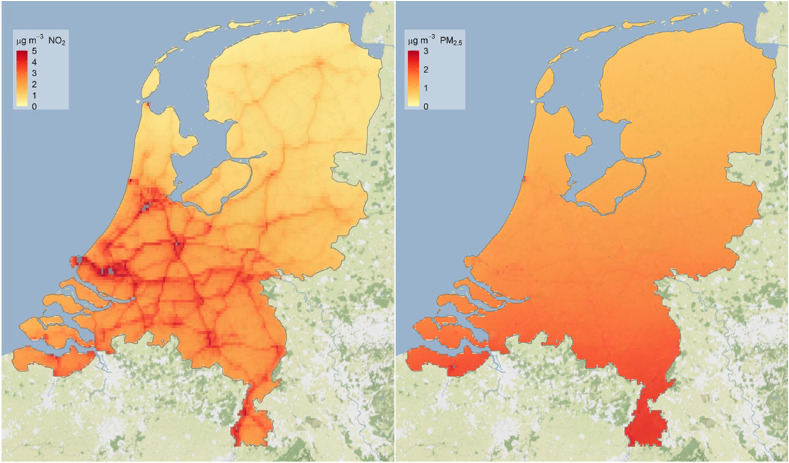
Using the EMEP model in its EMEP4NL configuration, the effect of the lockdown is estimated by comparing model simulations using lockdown scenarios with a reference scenario, both using the actual 2020 meteorology (see section 2.4). Fig. 7 shows the spatial distribution of the effect of the lockdown on the NO2 and PM2.5 concentrations. The largest effects are seen in the southern half of the country and for NO2, especially for the large cities and busy motorways. This coincides with the regions with the largest domestic emissions. For PM2.5 concentrations, the formation of secondary inorganic PM2.5 (nitrate, ammonium, and sulphate aerosols) and sources from abroad are responsible for a more homogeneous reduction in concentrations, which come on top of the reductions in domestic sources.
Fig. 7.
Calculated effect of the lockdown measures on the NO2 (left panel) and PM2.5 (right panel) concentrations (in μg m−3) at surface level in the Netherlands. The effect is calculated with the EMEP4NL model as the difference, over the lockdown period, between the high lockdown scenario and the reference scenario, at the lowest model layer.
The EMEP4NL simulated reductions are shown in Fig. 8 and Fig. A4 for rural and urban background measurement locations. The effects are shown for the low, high and extended lockdown scenario. The reductions in concentrations at the various stations are similar in magnitude for the PM10 and PM2.5 concentrations, consistent with the long-range character of particulate matter. The NOx, NO2, and O3 changes vary more in magnitude over the different stations. The average reductions for rural and urban background NO2 concentrations (Fig. 6) are about 8%, 18%, and 28%, for the low, high, and extended lockdown scenarios, respectively. Almost the same reductions are found in NOx concentrations. The reductions are smaller than found with the Random Forest analyses of the observations, especially for the urban background (see section 4). Only the reductions found with the extended lockdown scenario overlap partially with the uncertainty range of the Random Forest analyses. For two measurements stations, the modelled reductions deviate significantly from the Random Forest analyses, i.e., the Random Forest analyses show no significant decreases for the rural background station NL10934 and urban background station NL49014. Station NL10934 is in the far north of the Netherlands with no other stations nearby to verify the trend in the observed concentration. Station NL49014 is in downtown Amsterdam and the decreases in concentration for this station differ from the nearby station NL49003, probably because of local circumstances, such as local emissions, at the stations.
Much smaller reductions are found for PM10 concentrations, with about 5%, 10%, and 16%, for the low, high, and extended lockdown scenarios, respectively. These smaller reductions are in line with the smaller reductions found with the analyses of the observed concentrations. Larger reductions are modelled for PM2.5 concentrations; about 6%, 13%, and 20%, for the low, high, and extended lockdown scenarios, respectively. These reductions partially overlap with the Random Forest analyses. The observed decrease in PM2.5 concentrations shows a large variability with for some stations reductions of 45%, while for other stations reductions of less than 10%. The modelled reductions are similar in magnitude for all stations.
Modelled O3 concentrations show small increases in both the modelled scenarios and analyses of the observations. The modelled increases are on average about 2%, 3%, and 5%, for the low, high, and extended lockdown scenarios, respectively. The modelled increases show considerable variability in magnitude for the various locations. These increases again partially overlap with the Random Forest analyses.
The EMEP4NL model is also used to estimate the effects of the unusual 2020 meteorology on the concentrations alone. This is performed by comparing the modelled concentrations during the lockdown period in 2020 with the average modelled concentrations using the meteorology from 2017 to 2019, with both using the using the reference emission scenario. It is found that the 2020 meteorology during the lockdown period had a small effect on the NOx, NO2 and O3 concentrations. That is, the concentrations with 2020 meteorology are on average within 2% of the concentrations calculated with the meteorology of 2017–2019 (standard deviation (sd) of 13 percent point for NOx and NO2 and 4 percent point for O3). The unusual 2020 meteorology had a larger effect on the PM10 and PM2.5 concentrations. The 2020 meteorology resulted in on average 8% lower PM10 concentrations (sd of 8 percent point) than the concentrations calculated with the meteorology of 2017–2019 and 10% lower PM2.5 concentrations (sd of 11 percent point). So, the observed PM concentrations are reduced by the lockdown measures and by the unusual meteorology during the lockdown period in the Netherlands.
3.5. Reductions in traffic contributions
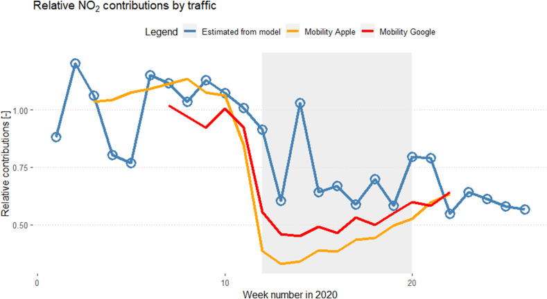
As described in section 2.5, RIVM produces hourly NO2 maps for the Netherlands which are calibrated using observations. One of the steps in the calibration is a scaling of the calculated NO2 traffic contributions using measurements at traffic locations that are influenced by traffic on roads in cities and highways. Fig. 9 shows the weekly average scaling factors in the calibration obtained for the months of January–May 2020. From week 12, a substantial drop in NO2 traffic concentration contributions is observed. Apart from week 14, the estimated NO2 contributions from traffic are about 65% of those in weeks 1–12, implying an average reduction of the concentration contributions from road traffic by about 35%.
Fig. 9.
Trend plot of estimated NO2 traffic contributions obtained from the hourly NO2 maps calculated in the Netherlands (blue). The red curves are mobility trend estimates reported by Apple (2020) and Google (2020). (For interpretation of the references to colour in this figure legend, the reader is referred to the Web version of this article.)
Mobility data provided by Apple (2020) and Google (2020) is also shown in Fig. 9. The trend shown in the mobility data of Apple and Google is quite similar to that estimated from the reduction in traffic contributions, although the drop in the latter is less pronounced.
The Netherlands Institute for Transport Policy Analysis reported in April 2020 that the number of transport movements in the Netherlands was reduced by some 55% due to the lockdown (KIM, 2020b). Some 39% of the people started working entirely from home, resulting in a significant reduction of traffic-related emissions. Using real-time information provided by the Netherlands National Data Warehouse for Traffic Information (NDW, 2020) we have estimated the change in traffic intensities and composition around the onset of the lockdown on three main highways in the Netherlands (the highways A1, A2 and A16). In the period of March 23 to April 5, 2020, the amount of light-duty traffic is reduced by 45–60% with respect to the average values of February 2020, whereas the number of middle-heavy and heavy-duty trucks is reduced by roughly 10% and 5%, respectively. Taking into account the different emission factors of these vehicles for NOx and NO2, we estimate a total effect on the NO2 concentration contributions of 35–40%. This estimate is quite close to the reduction in NO2 contributions observed in the calibration of the hourly maps.
4. Discussion
The EMEP4NL simulated reductions partially overlap with the Random Forest analyses when the 95% confidence intervals are considered, but especially for the extended lockdown scenario with relatively large assumed reductions in economic activities and corresponding emissions. There can be several reasons for the differences between both methods. 1) A Random Forest method is used to estimate what the concentrations would have been in the absence of reductions in emissions. The method uses a set of explanatory variables and historical observations to describe the concentrations. The whole difference between the observed 2020 concentrations and expected concentrations, in the absence of emission reductions, is ascribed to the lockdown measures. The effect of meteorological variability is at least mostly taken into account, but there might be other factors affecting the 2020 concentrations that have not been taken into account, which are now incorrectly ascribed to the lockdown measures. For example, changes in local emissions or the physical surroundings close to the measurement station. The unusual meteorological conditions during the lockdown might also not be present sufficiently in the training dataset used to estimate the Random Forest variables. Another potential source might be the absence of a trend term in the Random Forest analysis. NO2 concentrations at urban and traffic locations show a downward trend of about 1 μg m−3 per year. Ignoring a trend term could lead to an overestimation of the lockdown effect. Although when we included a trend term in additional Random Forest analysis the results hardly changed. Therefore, the effect of a trend term is probably small compared with the uncertainty derived by the Random Forest analysis. It is also not clear if a long-term trend will be relevant for the expected concentrations for a short period of only eight weeks. 2) Another reason explaining the difference between both methods could be an underestimation of the changes in economic activity and related emissions for the lockdown scenario. The scenario with extended emission reductions, i.e., reductions larger than based on the reported and estimated changed in economic activities (light and heavy-duty traffic and industry), is closest to the data from the Random Forest analyses. 3) The EMEP4NL model may not give a full explanation of measured PM concentrations.
Since a broader range of sources contributes to PM concentrations compared to nitrogen oxides, and the source contributions are transported over longer distances, the spatial gradients in PM concentrations are small (Fig. 7). PM2.5 reductions are smaller than those for NOx and NO2 due to the substantial contributions from secondary aerosols from the agricultural sector that are hardly affected by the lockdown. PM10 reductions are even less affected due to the contribution of natural sources such as windblown dust, sea salt, etc.
Increases are observed in O3 concentrations for all station types, but especially for traffic locations. Close to roads the emitted NO reacts with ozone to form NO2 (Parrish et al., 2012; van Pul et al., 2011). In the Netherlands, because of the high NOx emissions and corresponding concentrations, the concentrations of volatile organic compounds (VOCs) are the rate limiting step in the production of ozone at many locations. Reductions in NOx emissions therefore primarily lead to increases in O3.
Menut et al. (2020) reported effects of the lockdown measures on the air quality in Europe from simulations with an atmospheric chemistry-transport model and lockdown scenario for Western Europe. For the Netherlands, for the month of March, they found a reduction in NO2 concentration of 23% in urban areas and 16% in rural areas, a reduction in PM2.5 concentrations of 10% in rural and urban areas, and an increase in O3 concentrations of 6–8% in rural and urban areas. Their results for NO2 and O3 concentrations are similar to our findings, but are somewhat smaller than we what found for PM2.5 concentrations.
Reductions in NO2 tropospheric column values from satellite observations are reported by Bauwens et al. (2020). For cities as Frankfurt, Hamburg, and Brussels they report reductions in column NO2 amounts of about 20% during the lockdown. No data is reported for the Netherlands, but the reductions found for the cities in Belgium and Germany are close to our findings for NO2 surface concentrations.
Giani et al. (2020) analysed observations of PM2.5 concentrations and reported an average reduction of 17% for the whole of Europe. This average reduction is in line with the reductions we report here for the Netherlands. But, because of the large differences in the stringency of the lockdown measures in European countries and regional differences in meteorological conditions across Europe, the average value for Europe may not be representative for the Netherlands.
5. Conclusions
The Random Forest analysis of the observed concentrations and the EMEP4NL simulations with prescribed emission reductions yield similar changes in concentrations resulting from the lockdown measures in March to May 2020. The Random Forest analyses of the observations yield on average larger decreases in NOx, NO2, and PM2.5 concentration and larger increases in O3 concentration than the EMEP4NL simulations.
The Random Forest analyses yields reduction in NO2 concentrations of on average 30% (95% CI 25–35%), 26% (95% CI 21–32%), and 18% (95% CI 10–25%) for traffic, urban and rural background locations, respectively. Slightly smaller reductions of 8–28% are found with the EMEP4NL model for urban and regional locations with estimates of reductions in economic activity and emissions of traffic and industry in the Netherlands and other European countries. Reductions in observed PM2.5 concentrations of about 20% (10–25%) are found for all locations, which is again somewhat smaller estimates of 5–16% based on the model simulations.
From the analyses of the observations and the model simulations it can be concluded that the unusual 2020 meteorology in the Netherlands affected (decreased) PM10 and PM2.5 concentrations by about 8% and 10%, respectively, but not the NOx, NO2, and O3 concentrations. Therefore, the observed PM concentrations during the lockdown period are reduced by both the lockdown measures and by the 2020 meteorology.
The largest changes in economic activities during the lockdown period are for light-duty traffic. Based on a comparison between observed concentrations and modelled local traffic contributions along city roads and highways we derived a reduction in NO2 contributions from road traffic of about 35% during the lockdown, which is close to estimates of the reductions in traffic volumes.
Finally, it is important to note that the largest health effects from poor air quality in the Netherlands are associated with exposure to PM10 and PM2.5, and that exposure to NO2 contributes about one-third to the health effects in the Netherlands (Fischer et al., 2015). Also, the health effects are derived for a long-term (many years) exposure and it is not known what the long-term effects are for reductions for just a few months. Therefore, the lockdown measures in spring of 2020 have improved the air quality in the Netherlands, but the most important compounds for health effects have only been reduced by about 10–25%. By the middle of October, a second partial lockdown was announced with potentially additional positive effects on the air quality.
CRediT authorship contribution statement
Guus J.M. Velders: Conceptualization, Formal analysis, Investigation, Methodology, Supervision, Visualization, Writing - original draft, Writing - review & editing. Saskia M. Willers: Conceptualization, Data curation, Formal analysis, Investigation, Methodology, Validation, Writing - original draft, Writing - review & editing. Joost Wesseling: Conceptualization, Data curation, Formal analysis, Investigation, Methodology, Validation, Writing - original draft, Writing - review & editing. Sef van den Elshout: Investigation, Methodology, Validation, Writing - original draft. Eric van der Swaluw: Data curation, Formal analysis, Investigation, Writing - original draft. Dennis Mooibroek: Data curation, Formal analysis, Investigation, Methodology, Validation, Visualization, Writing - original draft. Sjoerd van Ratingen: Data curation, Formal analysis, Investigation, Writing - original draft.
Declaration of competing interest
The authors declare that they have no known competing financial interests or personal relationships that could have appeared to influence the work reported in this paper.
Footnotes
Supplementary data to this article can be found online at https://doi.org/10.1016/j.atmosenv.2020.118158.
Appendix A. Supplementary data
The following is the Supplementary data to this article:
References
- Alimissis A., Philippopoulos K., Tzanis C.G., Deligiorgi D. Spatial estimation of urban air pollution with the use of artificial neural network models. Atmos. Environ. 2018;191:205–213. doi: 10.1016/j.atmosenv.2018.1007.1058. [DOI] [Google Scholar]
- Apple Mobility trend reports. 2020. https://www.apple.com/covid19/mobility
- Bauwens M., Compernolle S., Stavrakou T., Müller J.-F., van Gent J., Eskes H., Levelt P.F., van der A R., Veefkind J.P., Vlietinck J., Yu H., Zehner C. Impact of coronavirus outbreak on NO2 pollution assessed using TROPOMI and OMI observations. Geophys. Res. Lett. 2020 doi: 10.1029/2020GL087978. 2020GL087978. [DOI] [PMC free article] [PubMed] [Google Scholar]
- Breiman L. Random forest. Mach. Learn. 2001;45:5–32. doi: 10.1023/A:1010933404324. [DOI] [Google Scholar]
- Carslaw D.C., Ropkins K. Openair — an R package for air quality data analysis. Environ. Model. Software. 2012;27:52–61. doi: 10.1016/j.envsoft.2011.1009.1008. [DOI] [Google Scholar]
- CEIP . Centre on Emission Inventories and Projections, EMEP/CEIP; Vienna, Austria: 2020. WebDab EMEP Emission Database. [Google Scholar]
- Cole M.A., Elliott R.J.R., Liu B. The impact of the Wuhan Covid-19 lockdown on air pollution and health: a machine learning and augmented synthetic control approach. Environ. Resour. Econ. 2020;76:553–580. doi: 10.1007/s10640-020-00483-4. [DOI] [PMC free article] [PubMed] [Google Scholar]
- DCMR . DCMR Environmental Protection Agency; Schiedam, the Netherlands: 2020. Air Quality Monitoring Network. [Google Scholar]
- DerSimonian R., Laird N. Meta-analysis in clinical trials. Contr. Clin. Trails. 1986;7:177–188. doi: 10.1016/0197-2456(86)90046-2. [DOI] [PubMed] [Google Scholar]
- Draxler R.R., Hess G.D. An overview of the HYSPLIT_4 modelling system for trajectories, dispersion, and deposition. Aust. Meteorol. Mag. 1998;47:295–308. [Google Scholar]
- EEA . European Environment Agency; Copenhagen, Denmark: 2019. Air Quality in Europe Report - 2019 Report. EEA Report No 10/2019. [Google Scholar]
- EMEP . Norwegian Meteorological Institute, EMEP MSC-W & CCC & CEIP, EMEP status report 1/2020, ISSN 1504-6192; Blinderd, Norway: 2020. Transboundary Particulate Matter, Photo-Oxidants, Acidifying and Eutrophying Compounds, Status Report 1/2020. [Google Scholar]
- EMEP/MSC-W . Norwegian Meteorological Institute, MSC-W Data Note 1/2020, ISSN 1890-0003; Netherlands: 2020. (Transboundary Air Pollution by Sulphur, Nitrogen, Ozone and Particulate Matter in 2018). Blinderd, Norway. [Google Scholar]
- Feng R., Zheng H., Gao H., Zhang A., Huang C., Zhang J., Luo K., Fan J. Recurrent Neural Network and random forest for analysis and accurate forecast of atmospheric pollutants: a case study in Hangzhou, China. J. Clean. Prod. 2018;231:1005–1015. doi: 10.1016/j.jclepro.2019.1005.1319. [DOI] [Google Scholar]
- Fischer P.H., Marra M., Ameling C.B., Hoek G., Beelen R., de Hoogh K., Breugelmans O., Kruize H., Janssen N.A.H., D H. Air Pollution and mortality in seven million adults: the Dutch environmental longitudinal study (DUELS) Environ. Health Perspect. 2015;123:697–704. doi: 10.1289/ehp.1408254. [DOI] [PMC free article] [PubMed] [Google Scholar]
- GGD . GGD Amsterdam; Amsterdam, the Netherlands: 2020. Air Quality Monitoring Network Amsterdam. [Google Scholar]
- Giani P., Castruccio S., Anav A., Howard D., Hu W., Crippa P. Short-term and long-term health impacts of air pollution reductions from COVID-19 lockdowns in China and Europe a modelling study. Lancet Planet. Health. 2020;4:e474–482. doi: 10.1016/S2542-5196(20)30224-2. [DOI] [PMC free article] [PubMed] [Google Scholar]
- Google . 2020. COVID-19 Community Mobility Reports.https://www.google.com/covid19/mobility/data_documentation.html?hl=en [Google Scholar]
- Grange S.K. 2018. Rmweather: Tools to Conduct Meteorological Normalisation on Air Quality Data.https://CRAN.R-project.org/package=rmweather R package version 0.1.2. [Google Scholar]
- Grange S.K., Carslaw D.C. Using meteorological normalisation to detect interventions in air quality time series. Sci. Total Environ. 2019;653:578–588. doi: 10.1016/j.scitotenv.2018.10.344. [DOI] [PubMed] [Google Scholar]
- Hoogerbrugge R., Geilenkirchen G.P., den Hollander H.A., van der Swaluw E., Visser S., de Vries W.J., Wichink Kruit R.J. National Institute for Public Health and the Environment; Bilthoven, the Netherlands: 2019. Large-scale Air Quality Concentration and Deposition Maps in the Netherlands. Report 2019. RIVM Report 2010-0091. [Google Scholar]
- Janssen S., Dumont G., Fierens F., Mensink C. Spatial interpolation of air pollution measurements using CORINE land cover data. Atmos. Environ. 2008;42:4884–4903. [Google Scholar]
- KIM . 2020. Coronacrisis Rem Op Wegverkeer.https://www.kimnet.nl/actueel/nieuws/2020/04/15/coronacrisis-rem-op-wegverkeer April 15, 2020. [Google Scholar]
- KIM . 2020. Mobiliteit en de coronacrisis.https://www.kimnet.nl/publicaties/rapporten/2020/04/20/mobiliteit-en-de-coronacrisis [Google Scholar]
- KNMI . KNMI; De Bilt, The Netherlands: 2020. Klimatologie - Informative over Weer in Het Verleden. [Google Scholar]
- Kuenen J.J.P., Visschedijk A.J.H., Jozwicka M., Denier van der Gon H.A.C. TNO-MACC_II emission inventory; a multi-year (2003–2009) consistent high-resolution European emission inventory for air quality modelling. Atmos. Chem. Phys. 2014;14:10963–10976. doi: 10.15194/acp-14-10963-2014. [DOI] [Google Scholar]
- Lautenschlager F., Becker M., Kobs K., Steininger M., Davidson P., Krause A., Hotho A. OpenLUR: off-the-shelf air pollution modeling with open features and machine learning. Atmos. Environ. 2020;233:117535. doi: 10.1016/j.atmosenv.2020.117535. [DOI] [Google Scholar]
- Liu F., Page A., Strode S.A., Yoshida Y., Choi S., Zheng B., Lamsal L.N., Li C., Krotkov N.A., Eskes H., Van der A R., Veefkind P., Levelt P.F., Hauser O.P., Joiner J. Abrupt decline in tropospheric nitrogen dioxide over China after the outbreak of COVID-19. Sci. Adv. 2020;6 doi: 10.1126/sciadv.abc2992. [DOI] [PMC free article] [PubMed] [Google Scholar]
- LML . National Institute of Public Health and the Environment; Bilthoven, the Netherlands: 2020. National Air Quality Monitoring Network. [Google Scholar]
- MACC . European Community Horizon 2020; Brussels, Belgium: 2016. Final Report MACC-III Monitoring Atmospheric Composition and Climate 3. [Google Scholar]
- Menut L., Bessagnet B., Siour G., Mailler S., Pennel R., Cholakian A. Impact of lockdown measures to combat Covid-19 on air quality over western Europe. Sci. Total Environ. 2020;741:140426. doi: 10.1016/j.scitotenv.2020.140426. [DOI] [PMC free article] [PubMed] [Google Scholar]
- NCAR . National Centre for Atmospheric Research; Boulder, USA: 2020. Weather Research and Forecasting Model.https://www.mmm.ucar.edu/weather-research-and-forecasting-model [Google Scholar]
- NDW . 2020. National Data Warehouse for Traffic Information.https://www.ndw.nu/en/ [Google Scholar]
- Parrish D.D., Law K.S., Staehelin J., Derwent R., Cooper O.R., Tanimoto H., Volz-Thomas A., Gilge S., Scheel H.-E., Steinbacher M., Chan E. Long-term changes in lower tropospheric baseline ozone concentrations at northern mid-latitudes. Atmos. Chem. Phys. 2012;12:11485–11504. doi: 10.15194/acp-12-11485-2012. [DOI] [Google Scholar]
- PRTR . National Institute for Public Health and the Environment; Bilthoven, the Netherlands: 2020. Pollutant Release & Transfer Register.http://www.emissieregistratie.nl [Google Scholar]
- RIVM . 2020. Air Quality Forecast NO2.https://www.luchtmeetnet.nl/verwacht?component=NO2 [Google Scholar]
- Shi X., Brasseur G.P. The response in air quality to the reduction of Chinese economic activities during the COVID-19 outbreak. Geophys. Res. Lett. 2020 doi: 10.1029/2020GL088070. [DOI] [PMC free article] [PubMed] [Google Scholar]
- Simpson D., Benedictow A., Berge H., Bergström R., Emberson L.D., Fagerli H., Flechard C.R., Hayman G.D., Gauss M., Jonson J.E., Jenkin M.E., Nyíri A., Richter C., Semeena V.S., Tsyro1 S., Tuovinen J.-P., Valdebenito Á., Wind P. The EMEP MSC-W chemical transport model – technical description. Atmos. Chem. Phys. 2012;12:7825–7865. doi: 10.5194/acp-12-7825-2012. https://emep.int/mscw/ [DOI] [Google Scholar]
- Tong W., Hong H., Fang H. Decision forest: combing the predictions of multiple independent decision tree models. J. Chem. Inf. Comput. Sci. 2003;43:525–531. doi: 10.1021/ci020058s. [DOI] [PubMed] [Google Scholar]
- Van der Swaluw E., de Vries W., Sauter F., Kruit R.W., Vieno M., Fagerli H., Wind P., van Pul A. 2020. Trend Analysis of Reduced Nitrogen Components over the Netherlands with the EMEP4NL and OPS Model. submitted for publication. [Google Scholar]
- van Pul W.A.J., Fischer P.H., de Leeuw F.A.A.M., Maas R.J.M., Mooibroek D., van Noije T.P.C., Roemer M.G.M., Sterkenburg A. National Institute for Public Health and the Environment; Bilthoven. The Netherlands: 2011. Dossier Ozon 2011. RIVM Report No. 680151001. [Google Scholar]
- Velders G.J.M., Maas R.J.M., Geilenkirchen G.P., De Leeuw F.A.A.M., Ligterink N.E., Ruyssenaars P., De Vries W.J., Wesseling J.P. Effects of European emission reductions on air quality in The Netherlands and the associated health effects. Atmos. Environ. 2020;221:117109. doi: 10.1016/j.atmosenv.2019.117109. [DOI] [Google Scholar]
- Viechtbauer W. Conducting meta-analyses in R with the metafor package. J. Stat. Software. 2010;36:1–48. doi: 10.18637/jss.v18036.i18603. [DOI] [Google Scholar]
- Wesseling J.P., Van Velze K. National Institute of Public Health and the Environment; Bilthoven, The Netherlands: 2014. Technical Description of Standard Calculation Method 2 (SRM-2) for Air Quality Calculations. RIVM Report 2014-0109. [Google Scholar]
Associated Data
This section collects any data citations, data availability statements, or supplementary materials included in this article.


